
Using a Kalman Filter to Assimilate TRMM-Based Real-Time Satellite Precipitation Estimates over Jinghe Basin, China


Abstract
:
1. Introduction
2. Study Area and Data
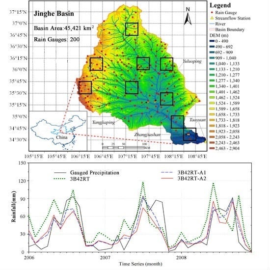
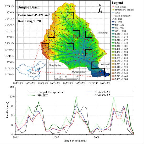
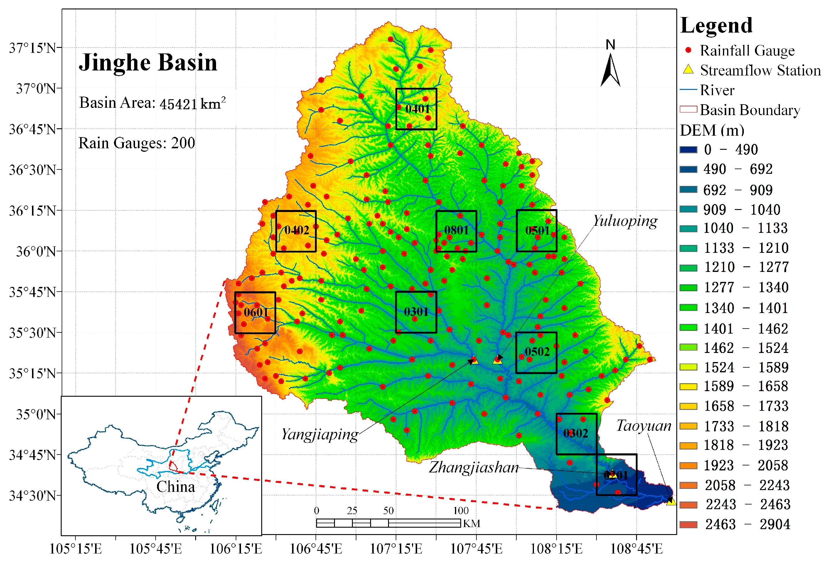
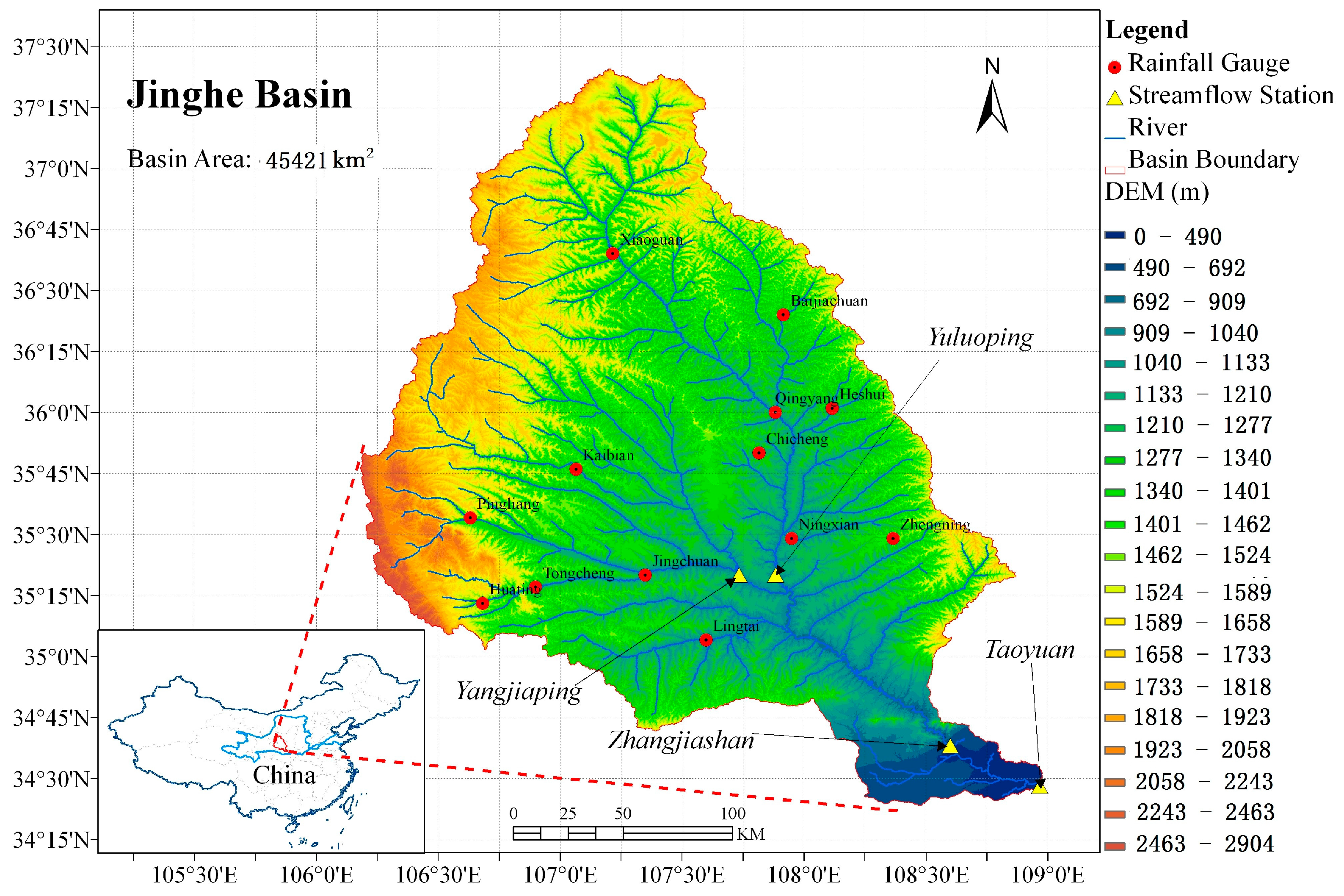
2.1. Jinghe Basin
2.2. NASA TMPA
3. Methodology
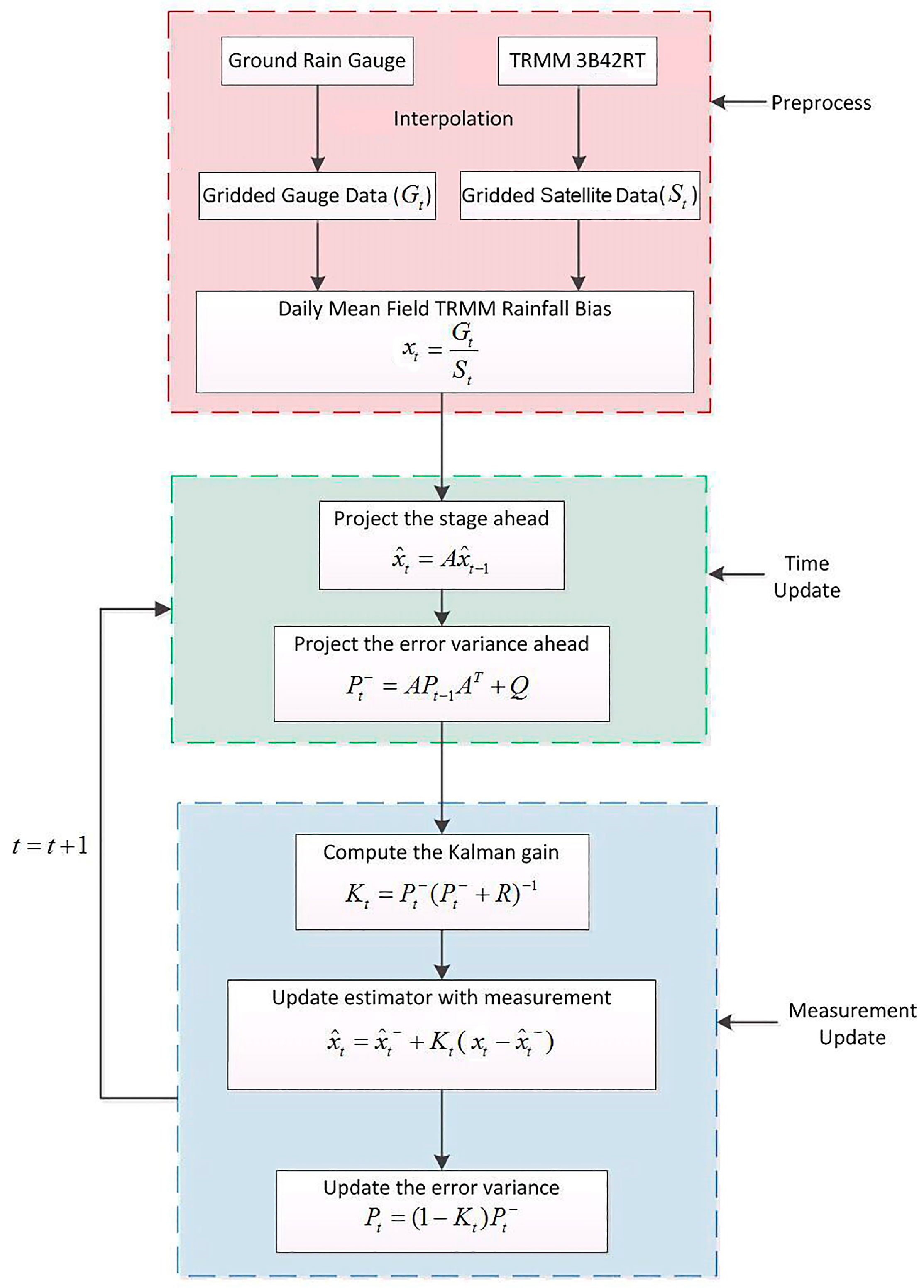
3.1. Preprocess
3.2. Time Update
3.3. Measurement Update
4. Results and Analysis
4.1. Implementation of Kalman Filter in Jinghe Basin
4.1.1. Basin-Averaged Comparison
4.1.2. Grid-Based Comparison
4.2. Assimilation Results with Sparse Gauges
4.3. Seasonal Analysis
4.4. Discussion
5. Summary
- (1)
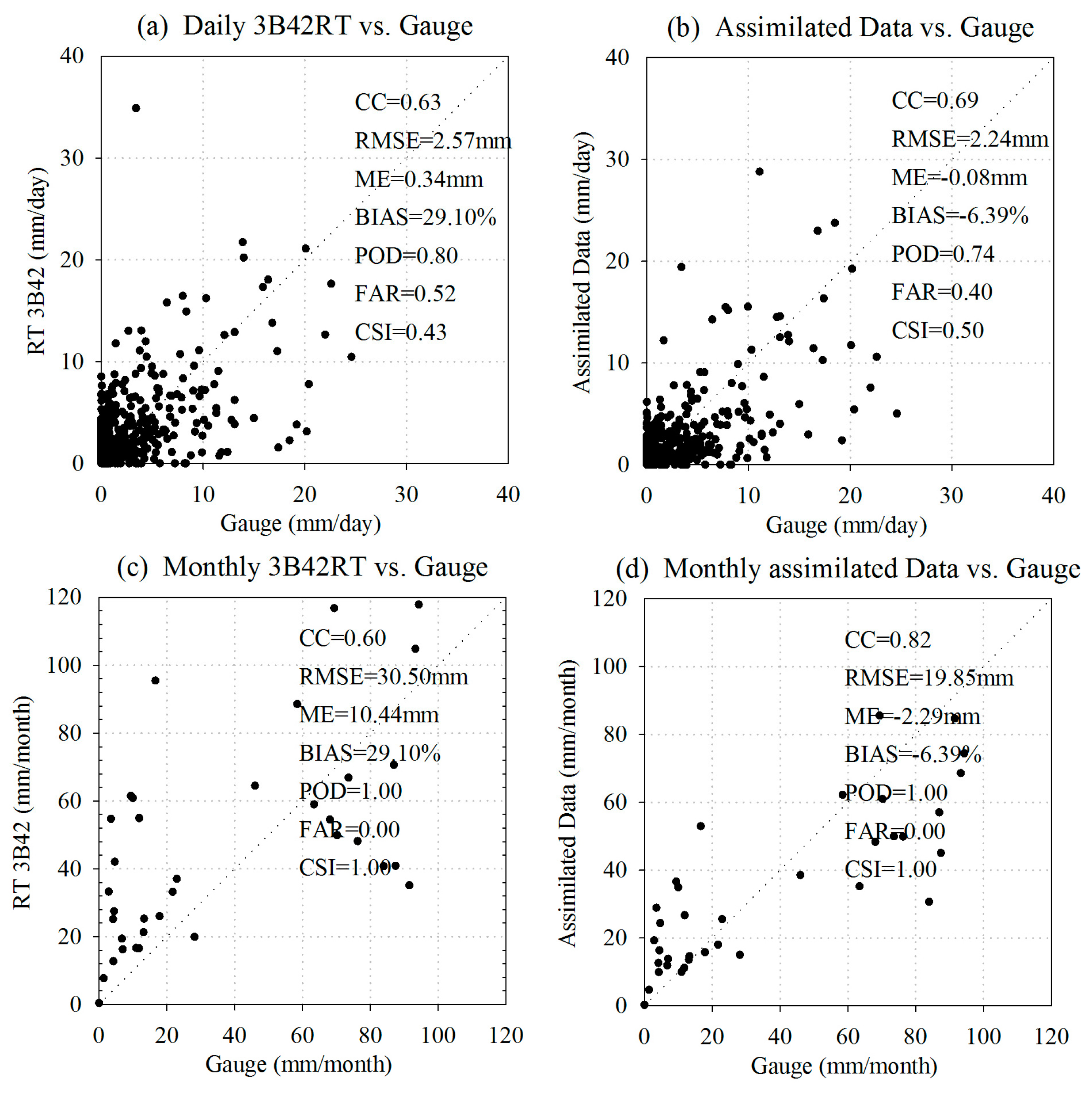
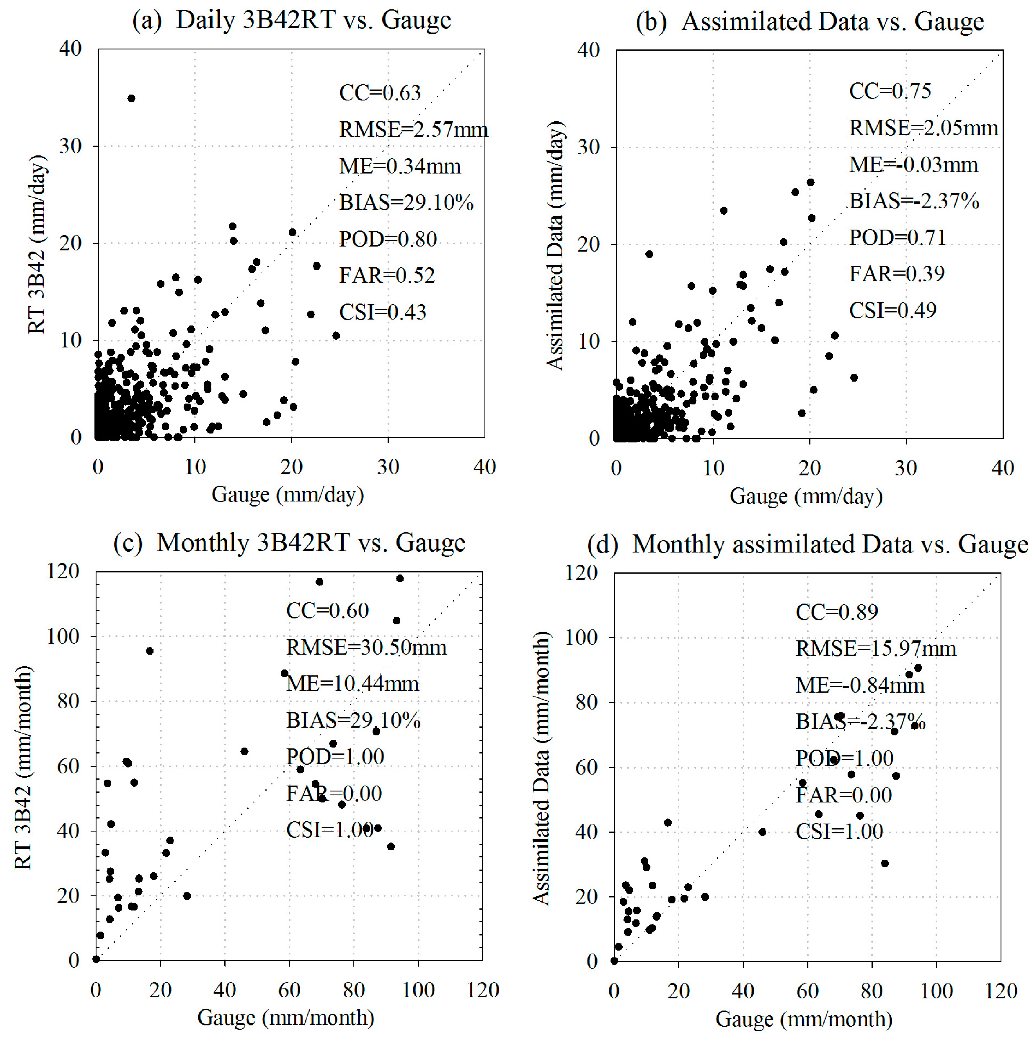
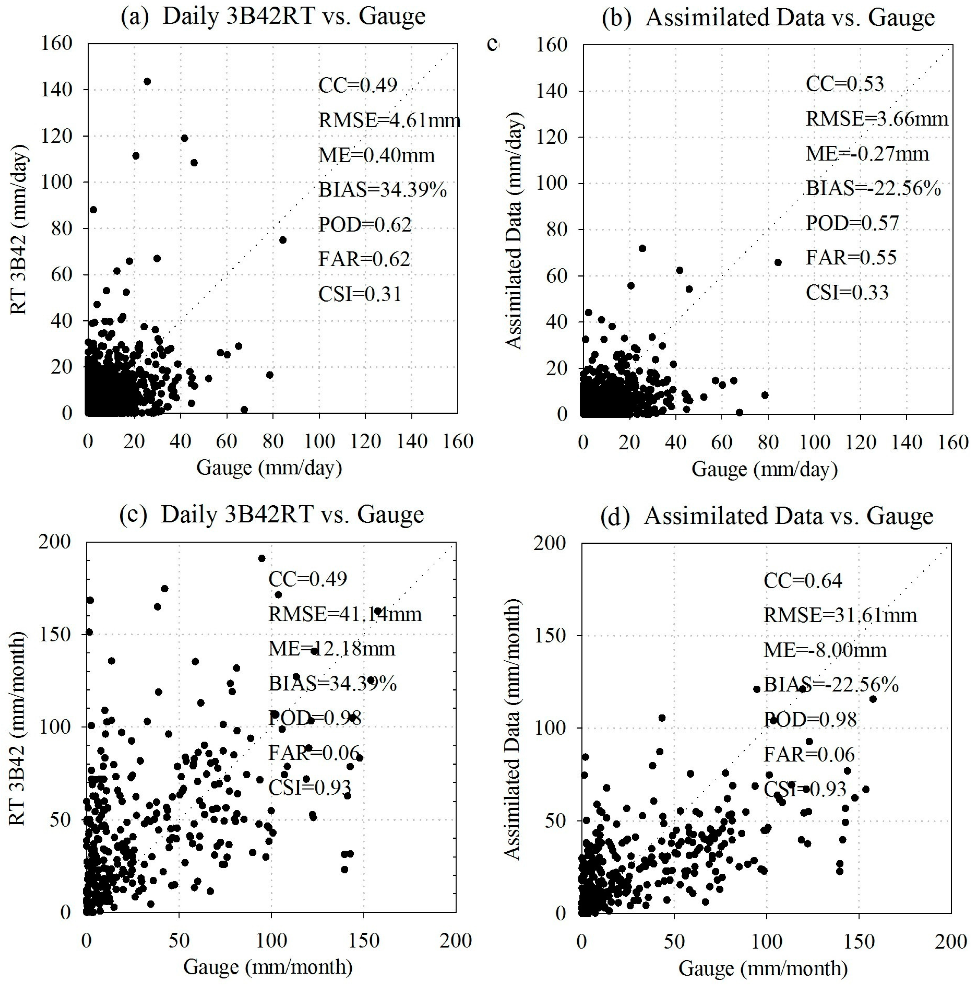
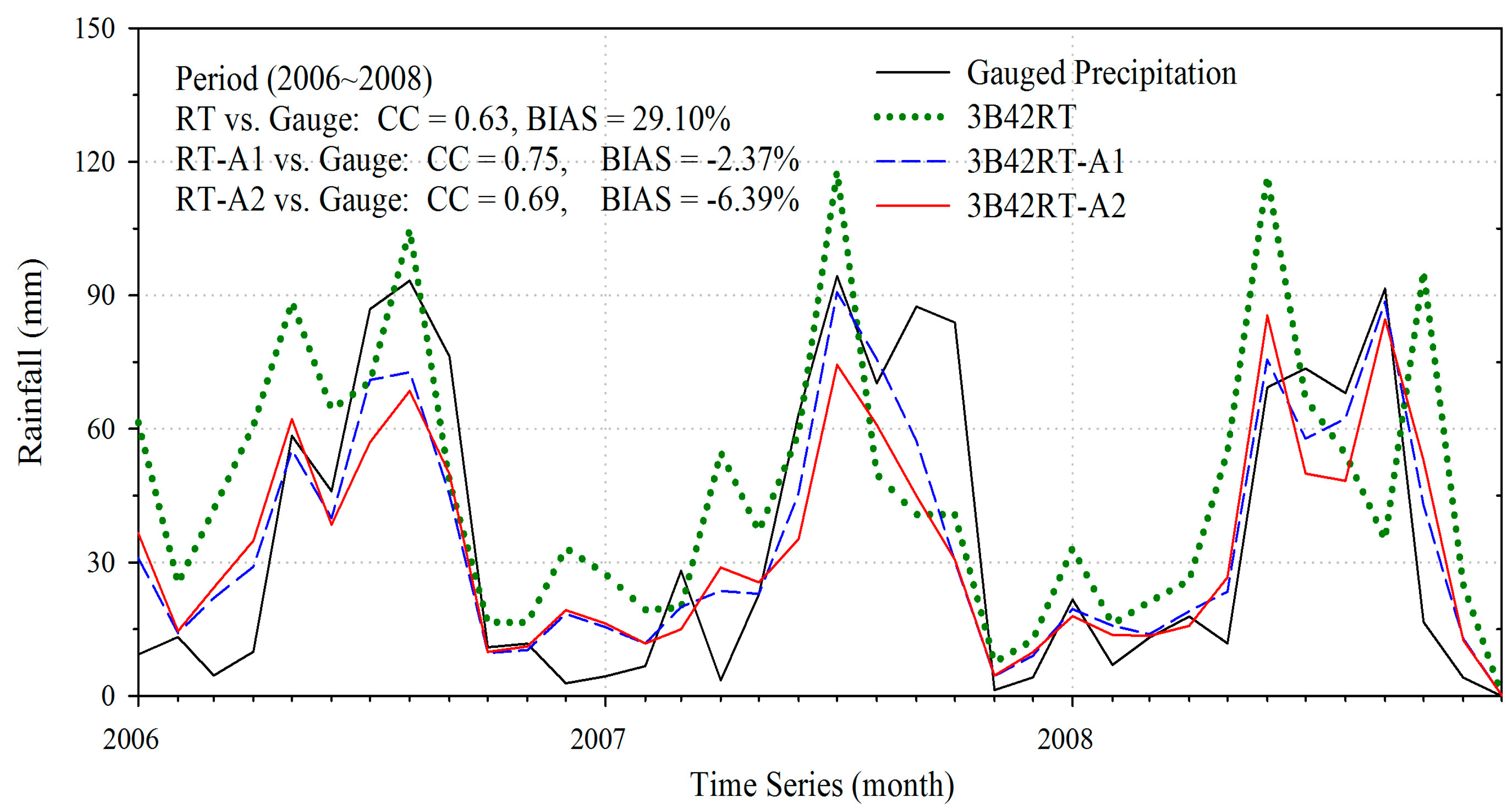
- Relative to gauge observations, the satellite precipitation estimation 3B42RT shows a large positive bias in the study basin. The results of our numerical experiments indicate that the assimilated precipitation estimates with Kalman filtering approach significantly outperform the original 3B42RT product before assimilation, even when the number of rain gauges used in the assimilation is fairly limited. Therefore, we concluded that the Kalman filter assimilation has great potential to improve the data accuracy of purely satellite precipitation retrievals, especially over the data sparse area.
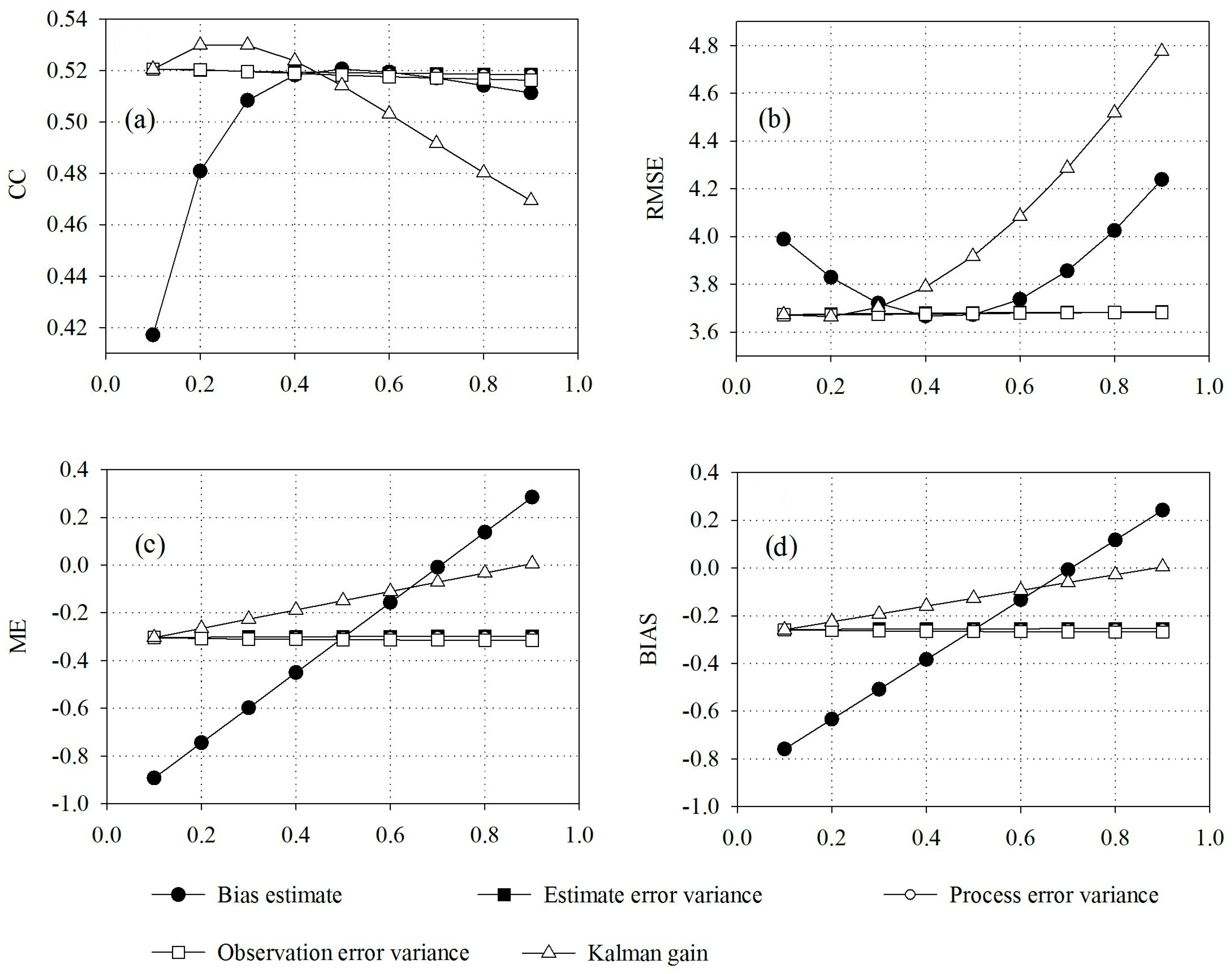
- (2)
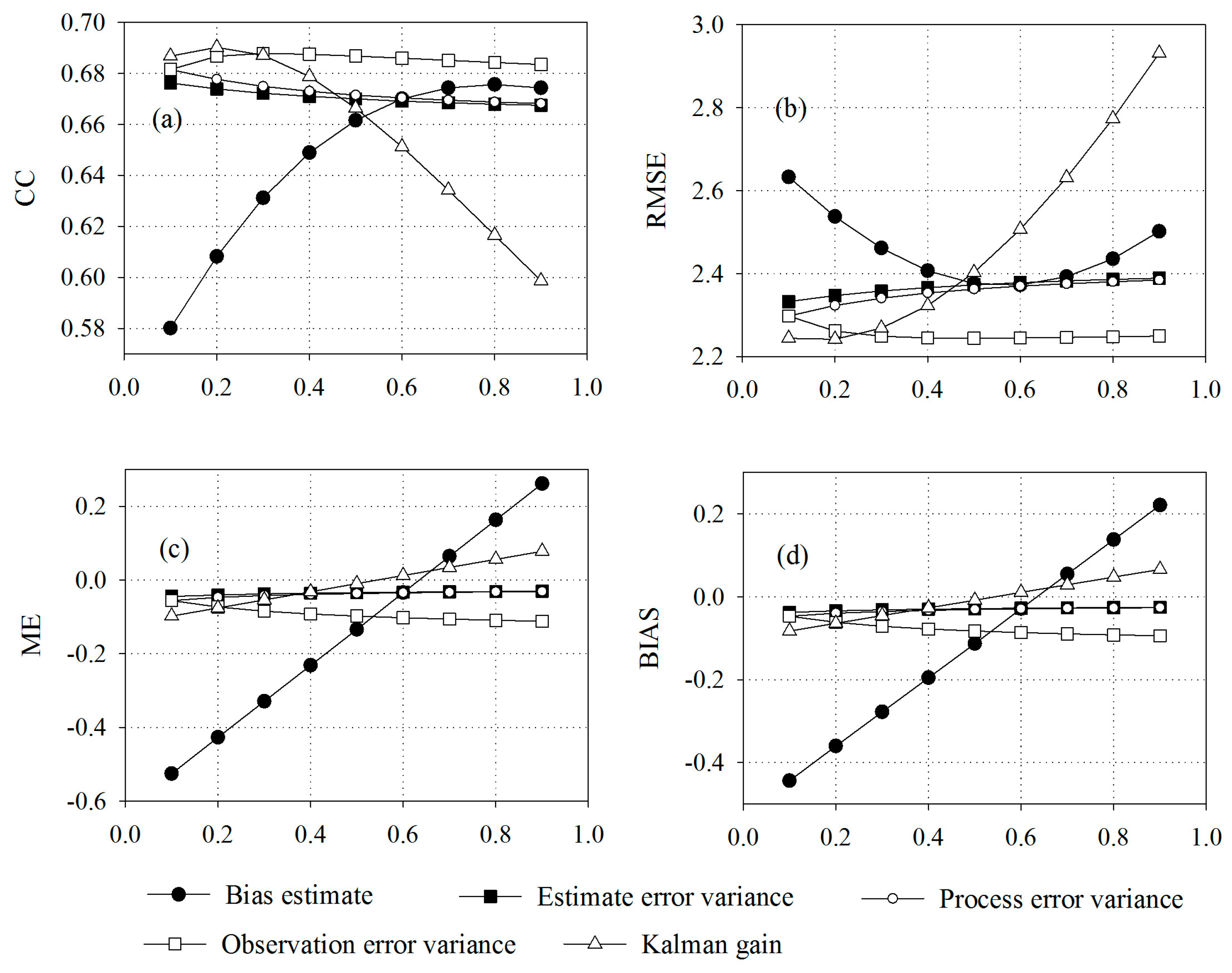
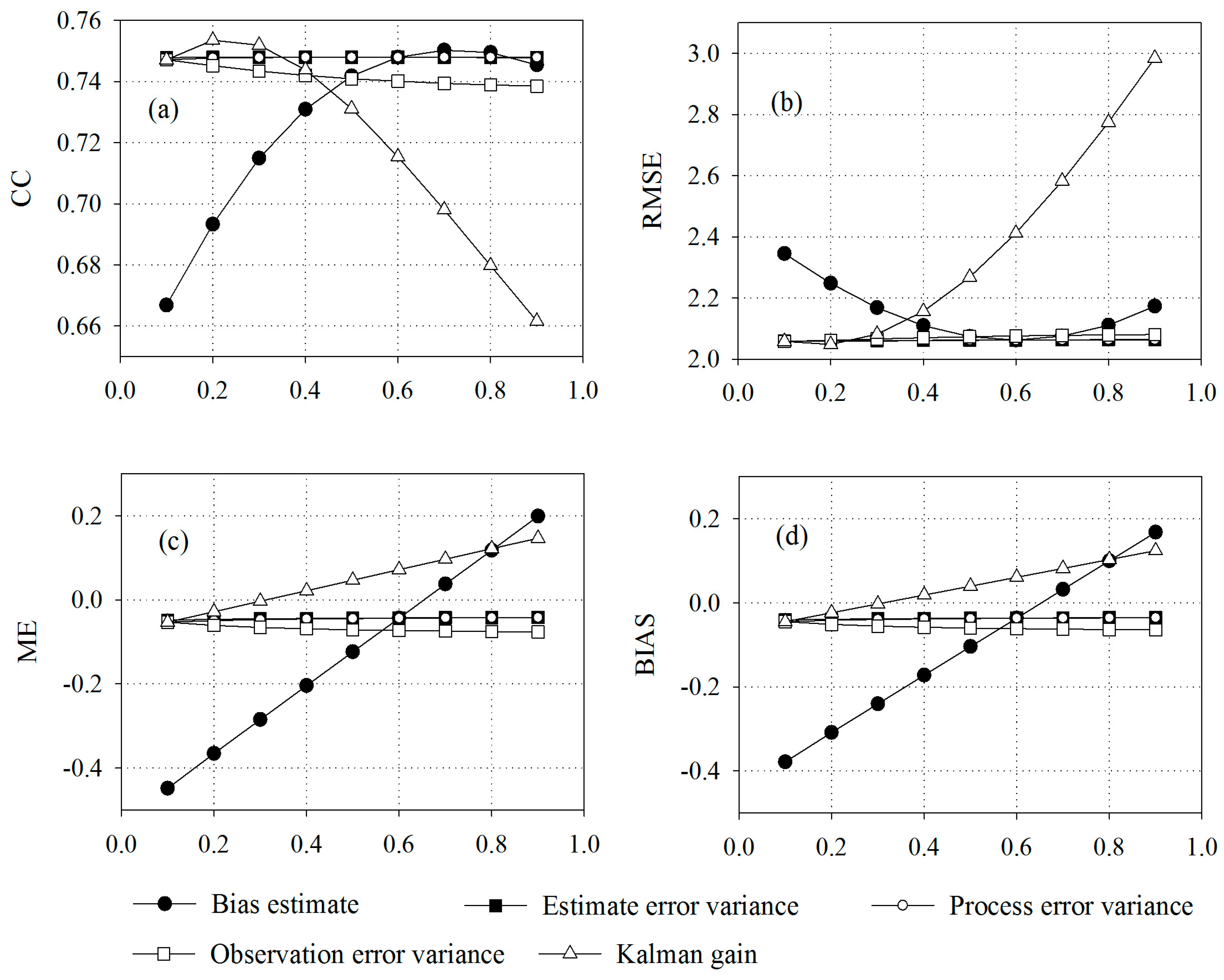
- The sensitivities of five Kalman filter parameters are analyzed for further understanding the assimilation process. Our analysis shows that two most sensitive parameters in the assimilation are mean field bias () and Kalman gain (), respectively, while other three parameters, i.e., estimate error variance (), observation error variance (), and process error variance (), have less sensitivity. It should be noted that the bias of four seasons seems to be averaged after assimilation. This might be caused by the continuous assimilation on multi-year time scales, which results in the homogenization of the statistical properties. This might be also the reason that causes the insensitivity of parameters R and Q. If the same assimilation method is solely applied for summer rainstorms, such situation might be changed.
- (3)
- In addition, our assessment illustrates that the Kalman filter seems to perform rather well in autumn, in which it can effectively reduce the error and bias of original 3B42RT and improve the skill of detecting rainy events. However, we have to note that the assimilation results in summer become relatively worse. The seasonal analysis and comparison with high and low density assimilation estimates also display that the situation of other seasons is obviously different from that in summer. For example, the RMSEs of low density assimilation were reduced by 3.40%, 4.27%, 3.96%, for spring, autumn and winter, respectively, while the dramatic deterioration by 14.74% was occurred in summer.
Acknowledgments
Author Contributions
Conflicts of Interest
Appendix A. Inverse Distance Weighting (IDW) Interpolation Method
References
- Bart, N.; Lettenmaier, D.P. Effect of precipitation sampling error on simulated hydrological fluxes and states: Anticipating the global precipitation measurement satellites. J. Geophys. Res. 2004, 109, 265–274. [Google Scholar]
- Heistermann, M.; Kneis, D. Benchmarking quantitative precipitation estimation by conceptual rainfall-runoff modeling. Water Resour. Res. 2011, 47, 667–671. [Google Scholar] [CrossRef]
- Sorooshian, S.; AghaKouchak, A.; Arkin, P.; Eylander, J.; Foufoula Georgiou, E.; Harmon, R.; Hendrickx, J.M.H.; Imam, B.; Kuligowski, R.; Skahill, B.; et al. Advanced concepts on remote sensing of precipitation at multiple scales. Bull. Am. Meteorol. Soc. 2011, 92, 1353–1357. [Google Scholar] [CrossRef]
- Huffman, G.J.; Adler, R.F.; Morrissey, M.; Bolvin, D.T.; Curtis, S.; Joyce, S.; McGavock, B.; Susskind, J. Global precipitation at one-degree daily resolution from multisatellite observations. J. Hydrometeorol. 2001, 2, 36–50. [Google Scholar] [CrossRef]
- Mishra, A.K.; Coulibaly, P. Developments in hydrometric network design: A review. Rev. Geophys. 2009, 47, 2415–2440. [Google Scholar] [CrossRef]
- Tian, Y.; Peters-Lidard, C.D.; Adler, R.F.; Kubota, T.; Ushio, T. Evaluation of GSMaP precipitation estimates over the contiguous United States. J. Hydrometeorol. 2010, 11, 566–574. [Google Scholar] [CrossRef]
- Zhang, J.; Howard, K.; Langston, C.; Vasiloff, S.; Kaney, B.; Arthur, A.; Cooten, S.V.; Kelleher, K.; Kitzmiller, D.; Ding, F.; et al. National Mosaic and Multi-sensor QPE (NMQ) System: Description, results, and future plans. Bull. Am. Meteorol. Soc. 2011, 92, 1321–1338. [Google Scholar] [CrossRef]
- Huffman, G.J.; Bolvin, D.T.; Nelkin, E.J.; Wolff, D.B.; Adler, R.F.; Gu, G.; Hong, Y.; Bowman, K.P.; Stocker, E.F. The TRMM Multisatellite Precipitation Analysis (TMPA): Quasi-global, multiyear, combined-sensor precipitation estimates at fine scales. J. Hydrometeor. 2007, 8, 38–55. [Google Scholar] [CrossRef]
- Huffman, G.J.; Adler, R.F.; Bolvin, D.T.; Gu, G. Improving the global precipitation record: GPCP version 2.1. Geophys. Res. Lett. 2009, 36, 153–159. [Google Scholar] [CrossRef]
- Joyce, R.J.; Janowiak, J.E.; Arkin, P.A.; Xie, P. CMORPH: A method that products global precipitation estimates from passive microwave and infrared data at high spatial and temporal resolution. J. Hydrometeor. 2004, 5, 487–503. [Google Scholar] [CrossRef]
- Hsu, K.L.; Gao, X.; Sorooshian, S.; Gupta, H.V. Precipitation Estimation from Remotely Sensed Information using Artificial Neural Networks. J. Appl. Meteorol. 1997, 36, 1176–1190. [Google Scholar] [CrossRef]
- Sorooshian, S.; Hsu, K.L.; Gao, X.; Gupta, H.V.; Imam, B.; Braithwaite, D. Evaluation of PERSIANN system satellite-based estimates of tropical rainfall. Bull. Am. Meteorol. Soc. 2000, 81, 2035–2046. [Google Scholar] [CrossRef]
- Kubota, T.; Shige, S.; Hashizume, H.; Ushio, T.; Aonashi, K.; Kachi, M.; Okamoto, K. Global precipitation map using satelliteborne microwave radiometers by the GSMaP project: Production and validation. IEEE Trans. Geosci. Remote Sens. 2007, 45, 2259–2275. [Google Scholar] [CrossRef]
- Hou, A.Y.; Kakar, R.K.; Neeck, S.; Azarbarzin, A.A.; Kummerow, C.D.; Kojima, M.; Oki, R.; Mura, K.N.; Iguchi, T. The global precipitation measurement mission. Bull. Am. Meteorol. Soc. 2014, 95, 701–722. [Google Scholar] [CrossRef]
- Tapiador, F.J.; Turk, F.J.; Petersen, W.; Hou, A.Y.; Garcia-Ortega, E.; Machado, L.A.T. Global precipitation measurement: Methods, datasets and applications. Atmos. Res. 2012, 104, 70–97. [Google Scholar] [CrossRef]
- Huffman, G.J.; Adler, R.F.; Bolvin, D.T.; Nelkin, E.J. The TRMM Multi-Satellite Precipitation Analysis (TMPA), Satellite Applications for Surface Hydrology; Springer: New York, NY, USA, 2010; pp. 3–22. [Google Scholar]
- Hossain, F.; Lettenmaier, D.P. Flood prediction in the future: Recognizing hydrologic issues in anticipation of the Global Precipitation Measurement mission. Water Resour. Res. 2006, 42, 973–977. [Google Scholar] [CrossRef]
- Hong, Y.; Adler, R.F.; Huffman, G.J. An Experimental Global Prediction System for Rainfall-triggered Landslides using Satellite Remote Sensing and Geospatial Datasets. IEEE Trans. Geosci. Remote Sens. 2007, 45, 1671–1680. [Google Scholar] [CrossRef]
- Yong, B.; Chen, B.; Gourley, J.J.; Ren, L.; Hong, Y.; Chen, X.; Wang, W.; Chen, S.; Gong, L. Intercomparison of the Version-6 and Version-7 TMPA precipitation products over high and low latitudes basins with independent gauge networks: Is the newer version better in both real-time and post-real-time analysis for water resources and hydrologic extremes? J. Hydrol. 2014, 508, 77–87. [Google Scholar]
- Li, L.; Hong, Y.; Wang, J.; Adler, R.F.; Policelli, F.S.; Habib, S.; Irwn, D.; Korme, T.; Okello, L. Evaluation of the real-time TRMM based multi-satellite precipitation analysis for an operational flood prediction system in Nzoia Basin, Lake Victoria, Africa. Nat. Hazards 2009, 50, 109–123. [Google Scholar] [CrossRef]
- Dinku, T.; Connor, S.J.; Seccato, P. Comparison of CMORPH and TRMM-3B42 over Mountainous Regions of Africa and South America Satellite, in Applications for Surface Hydrology; Springer: New York, NY, USA, 2010; pp. 193–204. [Google Scholar]
- Bitew, M.M.; Gebremichael, M. Evaluation of satellite rainfall products through hydrologic simulation in a fully distributed hydrologic model. Water Resour. Res. 2011, 47. [Google Scholar] [CrossRef]
- Hirpa, F.A.; Gebremichael, M.; Hopson, T. Evaluation of high resolution satellite precipitation products over very complex terrain in Ethiopia. J. Appl. Meteorol. Climatol. 2010, 49, 1044–1051. [Google Scholar] [CrossRef]
- Khan, S.I.; Hong, Y.; Wang, J.; Yilmaz, K.K.; Gourley, J.J.; Adler, R.F.; Brakenridge, G.R.; Policelli, F.; Habib, S.; Irwin, D. Satellite remote sensing and hydrologic modeling for flood inundation mapping in Lake Victoria Basin: Implications for hydrologic prediction in ungauged basins. IEEE Trans. Geosci. Remote Sens. 2011, 49, 85–95. [Google Scholar] [CrossRef]
- Su, F.; Gao, H.; Huffman, G.J.; Lettenmaier, D.P. Potential utility of the real-time TMPA-RT precipitation estimates in streamflow prediction. J. Hydrometeorol. 2011, 12, 444–455. [Google Scholar] [CrossRef]
- Tian, Y.; Peters-Lidard, C.D. Systematic anomalies over inland water bodies in satellite-based precipitation estimates. Geophys. Res. Lett. 2007, 34, 150–173. [Google Scholar] [CrossRef]
- Ebert, E.E.; Janowiak, J.E.; Kidd, C. Comparison of near-real-time precipitation estimates from satellite observations and numerical models. Bull. Am. Meteorol. Soc. 2007, 88, 47–64. [Google Scholar] [CrossRef]
- Gosset, M.; Viarre, J.; Quantin, G.; Alcoba, M. Evaluation of several rainfall products used for hydrological applications over West Africa using two high-resolution gauge networks. Q. J. R. Meteorol. Soc. 2013, 139, 923–940. [Google Scholar] [CrossRef]
- Pan, M.; Li, H.; Wood, E. Assessing the skill of satellite based precipitation estimates in hydrologic applications. Water Resour. Res. 2010, 46, 201–210. [Google Scholar] [CrossRef]
- Li, Z.; Yang, D.; Gao, B.; Jiao, Y.; Hong, Y.; Xu, T. Multiscale hydrologic applications of the latest satellite precipitation products in the Yangtze River Basin using a distributed hydrologic model. J. Hydrometeorol. 2015, 16, 407–426. [Google Scholar] [CrossRef]
- Lawson, W.G.; Hansen, J.A. Alignment error models and ensemble-based data assimilation. Mon. Weather Rev. 2005, 133, 1687–1709. [Google Scholar] [CrossRef]
- Tian, Y.; Peters-Lidard, C.D.; Eylander, J.B.; Joyce, R.J.; Huffman, G.J.; Adler, R.F.; Hsu, K.; Turk, F.; Garcia, M.; Zeng, J. Component analysis of errors in satellite-based precipitation estimates. J. Geophys. Res. Atmos. 2009, 114, 137–144. [Google Scholar] [CrossRef]
- Su, F.; Hong, Y.; Lettenmaier, D.P. Evaluation of TRMM Multisatellite Precipitation Analysis (TMPA) and its utility in hydrologic prediction in the La Plata basin. J. Hydrometeor. 2008, 9, 622–640. [Google Scholar] [CrossRef]
- Stisen, S.; Sandholt, I. Evaluation of remotesensing-based rainfall products through predictive capability in hydrological runoff modelling. Hydrol. Processes 2010, 24, 879–891. [Google Scholar] [CrossRef]
- Ciabatta, L.; Brocca, L.; Massari, C.; Moramarco, T.; Puca, S.; Rinollo, A.; Gabellani, S.; Wagner, W. Integration of satellite soil moisture and rainfall observations over the Italian territory. J. Hydrometeorol. 2015, 16, 1341–1355. [Google Scholar] [CrossRef]
- Kalman, R.E. A New Approach to Linear Filtering and Prediction Problems. J. Basic Eng. 1960, 82, 35–45. [Google Scholar] [CrossRef]
- Brown, R.G.; Hwang, P.Y.C. Introduction to Random Signals and Applied Kalman Filtering, 2nd ed.; John Wiley & Sons, Inc.: Hoboken, NY, USA, 1992. [Google Scholar]
- Ahnert, P.M. Kalman filter estimation of radar-rainfall mean field bias. In Proceedings of the 23rd Conference on Radar Meteorology and the Conference on Cloud Physics, Snowmass Village, CO, USA, 22–28 September 1986; pp. JP33–JP37.
- Smith, J.A.; Krajewski, W.F. Estimation of mean field bias of radar rainfall estimates. J. Appl. Meteorol. 1991, 30, 397–411. [Google Scholar] [CrossRef]
- Anagnostou, E.N.; Krajewski, W.F.; Seo, D.J.; Johnson, E.R. Mean-field rainfall bias studies for WSR-88D. J. Hydrol. Eng. 2012, 3, 149–159. [Google Scholar] [CrossRef]
- Seo, D.J.; Breidenbach, J.P.; Johnson, E.R. Real-time estimation of mean field bias in radar rainfall data. J. Hydrol. 1999, 223, 131–147. [Google Scholar] [CrossRef]
- Dinku, T.; Ananostou, E.N.; Borga, M. Improving radar based estimation of rainfall over complex terrain. J. Appl. Meteorol. 2002, 41, 1163–1178. [Google Scholar] [CrossRef]
- Chumchean, S.; Seed, A.; Sharma, A. Correcting of real-time radar rainfall bias using a Kalman filtering approach. J. Hydrol. 2006, 317, 123–137. [Google Scholar] [CrossRef]
- Hossain, F.; Huffman, G.J. Investigating error metrics for satellite rainfall at hydrologically relevant scales. J. Hydrometeorol. 2008, 9, 563–575. [Google Scholar] [CrossRef]
- Zimmerman, D.; Pavlik, C.; Ruggles, A.; Armstrong, M.P. An Experimental Comparison of Ordinary and Universal Kriging and Inverse Distance Weighting. Math. Geol. 1999, 31, 375–390. [Google Scholar] [CrossRef]
- Lu, G.Y.; Wong, D.W. An adaptive inverse-distance weighting spatial interpolation technique. Comput. Geosci. 2008, 34, 1044–1055. [Google Scholar] [CrossRef]
- Adler, R.F.; Huffman, G.J.; Chang, A.; Ferraro, R.; Xie, P.; Janowiak, J.; Rudolf, B.; Schneider, U; Curtis, S.; Bolvin, D.; et al. The version 2 Global Precipitation Climatology Project (GPCP) monthly precipitation analysis (1979–present). J. Hydrometeorol. 2003, 4, 1147–1167. [Google Scholar] [CrossRef]
- Chokngamwong, R.; Chiu, L. Thailand daily rainfall and comparison with TRMM products. J. Hydrometeorol. 2008, 9, 256–266. [Google Scholar] [CrossRef]


| OP | Experiment I | 0.6 | 0.1 | 0.1 | 0.1 | 0.2 |
| Experiment II | 0.4 | 0.1 | 0.1 | 0.2 | 0.2 | |
| Experiment III | 0.6 | 0.1 | 0.1 | 0.5 | 0.2 | |
| SR | Experiment I | 13.71% | 0.24% | 0.25% | 1.08% | 45.71% |
| Experiment II | 15.59% | 0.30% | 0.30% | 0.31% | 30.32% | |
| Experiment III | 10.97% | 2.43% | 3.77% | 2.39% | 30.78% | |
| CC | RMSE | BIAS | |||||
|---|---|---|---|---|---|---|---|
| RT | New | 3B42RT | New | 3B42RT | New | ||
| Spring | Basin Average (H) | 0.58 | 0.64 | 2.12 | 1.47 | 1.37 | 0.35 |
| Basin Average (L) | 0.58 | 0.63 | 2.12 | 1.52 | 1.37 | 0.45 | |
| Grid Based | 0.43 | 0.48 | 3.52 | 2.27 | 1.42 | 0.27 | |
| Summer | Basin Average (H) | 0.80 | 0.78 | 2.67 | 2.85 | 0.06 | −0.11 |
| Basin Average (L) | 0.80 | 0.69 | 2.67 | 3.27 | 0.06 | −0.22 | |
| Grid Based | 0.58 | 0.59 | 6.24 | 5.64 | 0.07 | −0.38 | |
| Autumn | Basin Average (H) | 0.32 | 0.74 | 3.55 | 2.34 | −0.15 | −0.21 |
| Basin Average (L) | 0.32 | 0.70 | 3.55 | 2.44 | −0.15 | −0.22 | |
| Grid Based | 0.35 | 0.48 | 5.30 | 3.74 | −0.07 | −0.40 | |
| Winter | Basin Average (H) | 0.18 | 0.24 | 1.49 | 1.01 | 2.29 | 0.95 |
| Basin Average (L) | 0.18 | 0.18 | 1.49 | 1.05 | 2.29 | 1.02 | |
| Grid Based | 0.12 | 0.11 | 2.43 | 1.69 | 2.27 | 0.81 | |
© 2016 by the authors; licensee MDPI, Basel, Switzerland. This article is an open access article distributed under the terms and conditions of the Creative Commons Attribution (CC-BY) license (http://creativecommons.org/licenses/by/4.0/).
Share and Cite
Chen, J.; Yong, B.; Ren, L.; Wang, W.; Chen, B.; Lin, J.; Yu, Z.; Li, N. Using a Kalman Filter to Assimilate TRMM-Based Real-Time Satellite Precipitation Estimates over Jinghe Basin, China. Remote Sens. 2016, 8, 899. https://doi.org/10.3390/rs8110899
Chen J, Yong B, Ren L, Wang W, Chen B, Lin J, Yu Z, Li N. Using a Kalman Filter to Assimilate TRMM-Based Real-Time Satellite Precipitation Estimates over Jinghe Basin, China. Remote Sensing. 2016; 8(11):899. https://doi.org/10.3390/rs8110899
Chicago/Turabian StyleChen, Jiaqi, Bin Yong, Liliang Ren, Weiguang Wang, Bo Chen, Jianan Lin, Zhongbo Yu, and Ning Li. 2016. "Using a Kalman Filter to Assimilate TRMM-Based Real-Time Satellite Precipitation Estimates over Jinghe Basin, China" Remote Sensing 8, no. 11: 899. https://doi.org/10.3390/rs8110899