Investigation of Snow Cover Effects and Attenuation Correction of Gamma Ray in Aerial Radiation Monitoring

Abstract

In aerial radiation monitoring (ARM), the air dose rate cannot be appropriately estimated under snowy conditions due to attenuation of gamma rays by the snow layer. A technique to address this issue is required for ARM to obtain enough signals for air dose rates. To develop this technique, we investigated the relationship between snow depth and ARM measurement results using ARM, laser imaging detection and ranging, and ground measurement before and after snowfall. From the measured data, the results obtained using three different correction factors were examined and compared. An appropriate correction improved the underestimation of the air dose rate. However, further improvement in the accuracy of the analysis requires accurate estimation of the snow water equivalent.

1. Introduction

The Great East Japan Earthquake on 11 March 2011 generated a series of large tsunami waves that resulted serious damage to the Fukushima Daiichi nuclear power station (FDNPS) and radionuclides were discharged to the environment. Immediately after the FDNPS accident, aerial radiation monitoring (ARM) began by the U.S. Department of Energy and the Japanese Ministry of Education, Culture, Sports Science and Technology to assess the air dose rate from deposited radioactive nuclides and to quantify the activity concentration [1,2,3]. The ARM has continued until the present time by the Nuclear Regulation Authority in Japan and the Japan Atomic Energy Agency [4]. The information about the temporal variation of the air dose rate became clear because the radiation distribution data by ARM within the 80 km radius from FDNPS was acquired nine times by April 2016. The results of the ARM are used as basic data for determination of the decontamination area and the evacuation order area by decision makers in Japan.

The ARM is suitable for the measurement of radiation distribution in the environment in a wide area at accidents of nuclear facilities. The basic technique of ARM was referred to in a report from an international organization [5]. However, actual parameters for data analysis have to be set in consideration of the topography and climatic condition of the targeted measurement area. Most of the area in Fukushima prefecture has snow in winter. In a situation of snow cover after the deposition of radionuclides, ARM cannot be used in snowfall areas because the shielding coefficient of the snow layer was not known. To prepare for future similar situations and enable ARM under snowy conditions, a method to correct the shielding effect by snow accurately must be developed for post-accident.

In this study, we evaluate the relationship between snow depth and gamma ray attenuation. In addition, a method of analysis of the air dose rate in snowy conditions is proposed and applied to actual measurement results. ARM was conducted to obtain the air dose rate before and after snowfall. In previous studies, the amount of snow in snow layers was measured using ARM to compare the amount of natural radiation before and after snowfall [6,7], and the decrease in personal dose was evaluated [8]. The shielding factor changes depending on snow water equivalent, SWE, which means the weight per unit area. In addition, SWE is obtained from snow depth and density. To achieve the purpose of this study, it is necessary to obtain the snow depth and density. They can be obtained by the ground measurement. However, because ARM is needed to measure a wide area rapidly, the measurements for snow depth and density also have to be measured in a wide area rapidly. In this study, to obtain snow depth, we performed laser imaging detection and ranging (LiDAR) [9,10,11] and ground measurement in parallel with ARM before and after snowfall. The snow density was obtained by the ground measurement result. By using these measured snow densities and depths, SWE was obtained. In addition, SWE was also obtained with the hydrological model and the meteorological data. Then, we corrected the air dose rate with SWE obtained with each approach and compared these results.

2. Materials and Methods

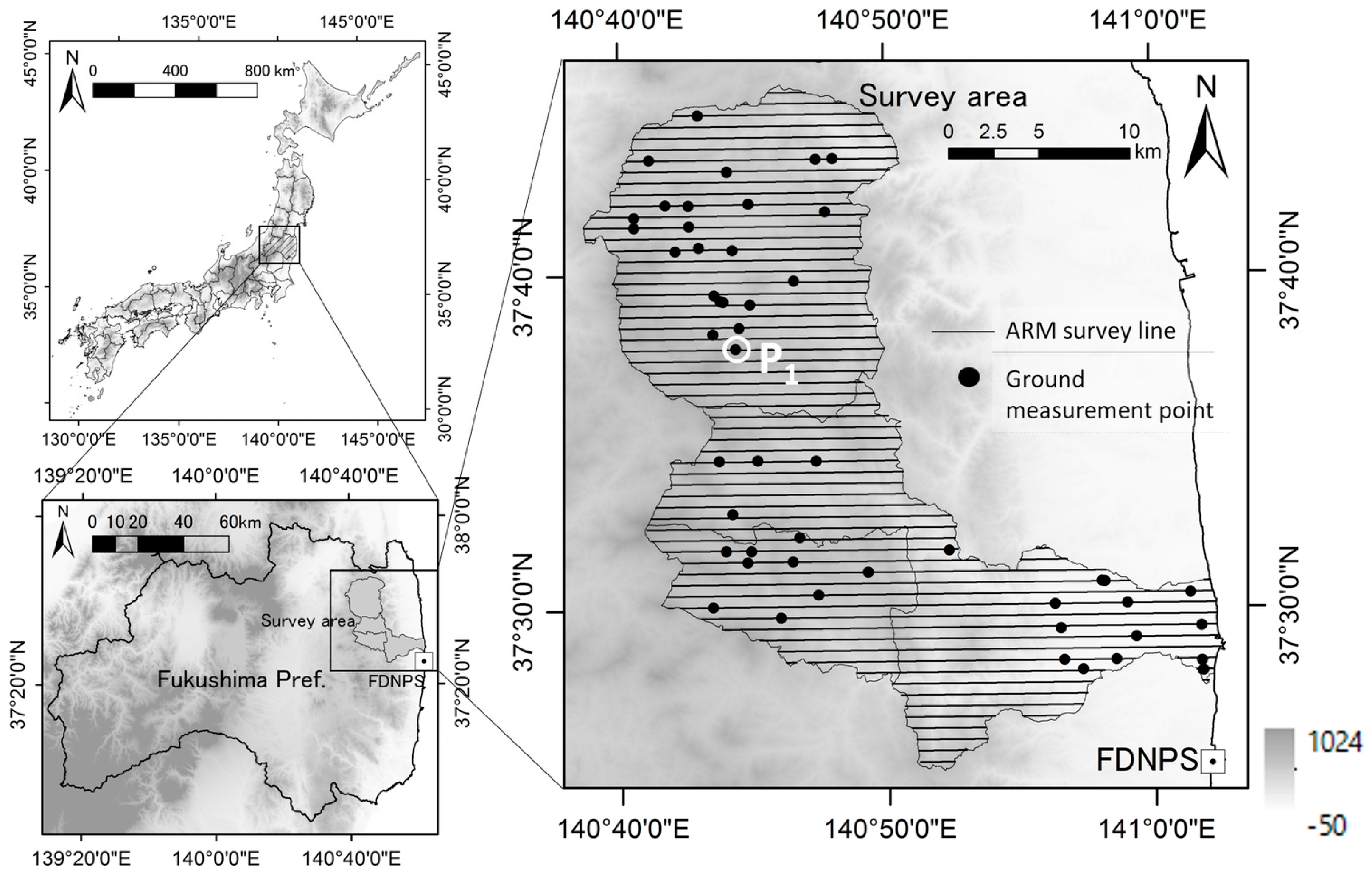
2.1. Measurement Area

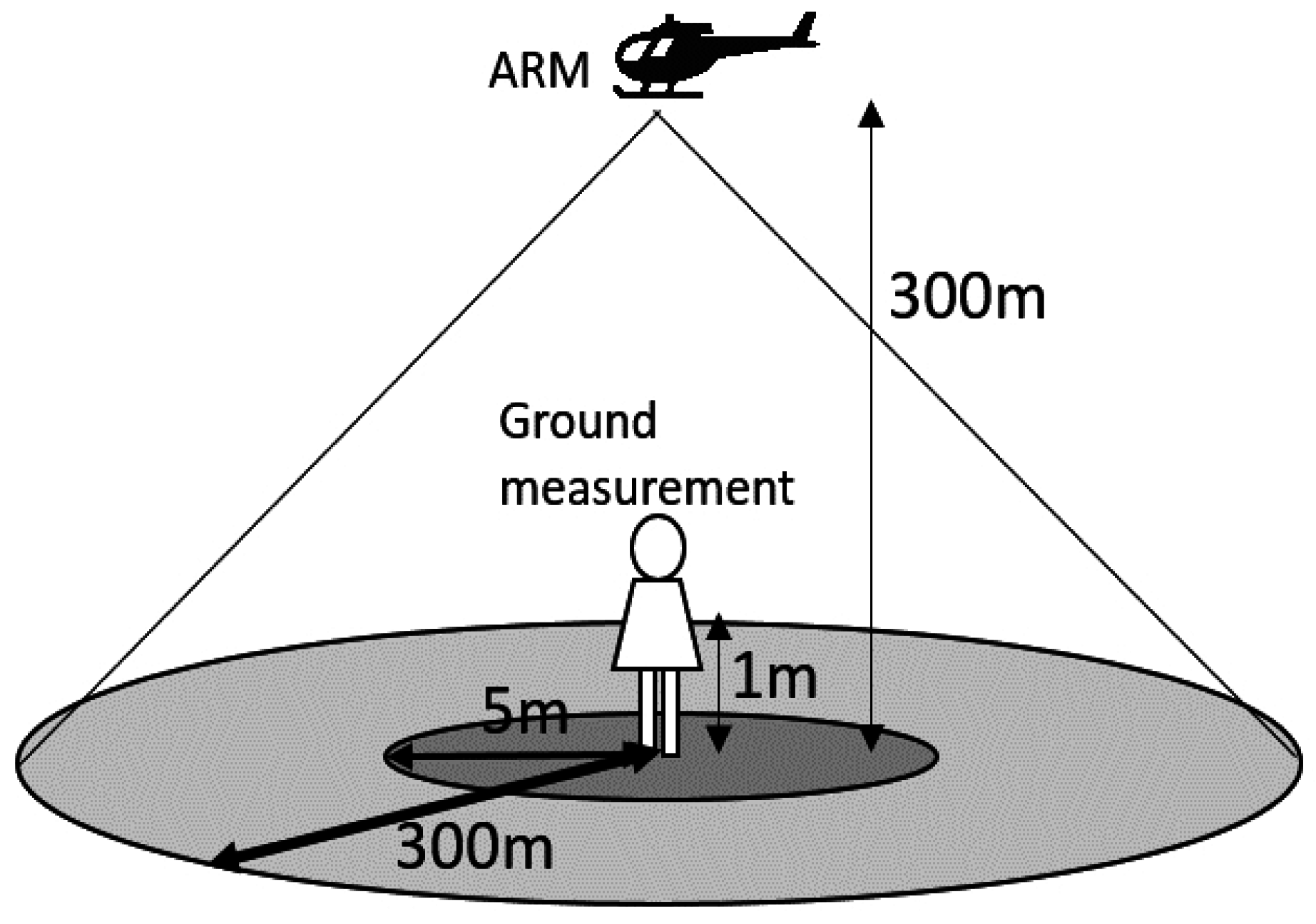
A manned helicopter was used to conduct ARM and LiDAR in an area of Fukushima prefecture in November 2015 (as the season before snowfall) and in February 2016 (as the season after snowfall in 2015). The survey area is shown in Figure 1. Essentially, the eastern region of the survey area is not subject to snow because it is warm along the coast. The ARM and LiDAR were conducted on the same day.

2.2. ARM

In the ARM, a helicopter was flown over the land surface at an altitude of 300 m above ground level. Eighty percent of the total contribution of gamma rays from the ground comes from the area within a 300 m radius just below the ARM measurement point as shown in Figure 2. The survey line was a comb-shaped pattern with intervals of 600 m.

The measurement system mounted inside the helicopter was fabricated by Radiation Solutions Inc. (Mississauga, ON, Canada). The system comprised two detection systems with three large NaI detectors (2 inch × 4 inch × 16 inch). The gamma-ray spectrum was acquired every 1 s, along with the positional information obtained using a GPS. From the spectrum, the net count rate, C_net (count per second), was obtained by subtracting the background count caused by cosmic rays. The background caused by cosmic rays, C_CR, was obtained using the cosmic-ray index, I_CR, [1] as shown in Figure 3. To calculate the I_CR, we collected a spectrum at a higher altitude of 1000 m above the ground or above the sea. In either case, the spectrum was collected without effects of natural nuclides. The spectrum was divided into two areas at an energy of 2800 keV. From the count rates in both areas, I_CR is defined as:

$$I_{CR}=\left(C_{<2800\mathrm{keV},CR}+C_{>2800\mathrm{keV},CR}\right)/C_{>2800\mathrm{keV},CR},$$

(1)

where C_{<2800 keV,CR} is the count rate below 2800 keV and C_>2800keV,CR is the count rate above 2800 keV. Using I_CR, we obtained C_CR as

$$C_{CR}=I_{CR}\times C_{>2800\mathrm{keV},m},$$

(2)

where C_{>2800 keV,m} is the count rate above 2800 keV measured in a survey flight.

By analyzing the net count rate, we obtained the air dose rate, D (μSv·h⁻¹) as

$$D=C_{net}\times CD/exp\left(AF\times \left(H_{std}-H\right)\right),$$

(3)

where CD is the dose rate conversion factor (μSv·h⁻¹·counts per second⁻¹), AF is the attenuation coefficient of gamma rays by air (m⁻¹), H_std is the standard altitude, which was determined as 300 m, and H is the flight altitude of the survey flight (m). These parameters were obtained from the test line measurement [1].

2.3. Ground Measurement

The air dose rate at 1 m above the ground was measured using a portable NaI survey meter (TCS-171B, Hitachi, Ltd., Mitaka, Japan) with a crystal size of φ25.4 × 25.4 mm, an energy resolution of ±15% for ¹³⁷Cs and an energy range from 50 keV to 3 MeV. Eighty percent of the total contribution of gamma rays from the ground originates from the area within a 5 m radius, as shown in Figure 2. In addition, the snow depth and snow weight were obtained by sampling at 52 points using a snow sampler. The sampling points are shown in Figure 1 as black points.

2.4. LiDAR

In LiDAR, the ground or snow layer surface was irradiated with a laser from a laser scanner mounted on the bottom of the helicopter. The elevation and landforms were surveyed on the basis of the distance to the ground calculated from the time lag of the reflected laser and on the basis of the positional information of the helicopter obtained using a GPS survey instrument and an internal measurement unit. In this study, the SAKURA system of the NAKANIHON Air Service Co. (Nagoya, Japan) was used. The flight conditions and the device configuration are shown in

Table 1. Flight condition and LiDAR device configuration (SAKURA system).

Parameter	Value
Flight altitude	450 m
Flight velocity	28 m/s
Frequency of laser firing	200 kHz before snowfall 100 kHz after snowfall
Scan frequency	75 Hz
Scan angle	±30°
Wave length of laser	1550 nm
Resolution of target	0.5 m
Precision of elevation	7 cm

. LiDAR was performed before and after snowfall, and digital elevation models (DEMs) were created. By subtracting both DEMs obtained from LiDAR, we obtained the snow depth, t.

3. Results

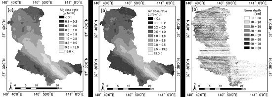
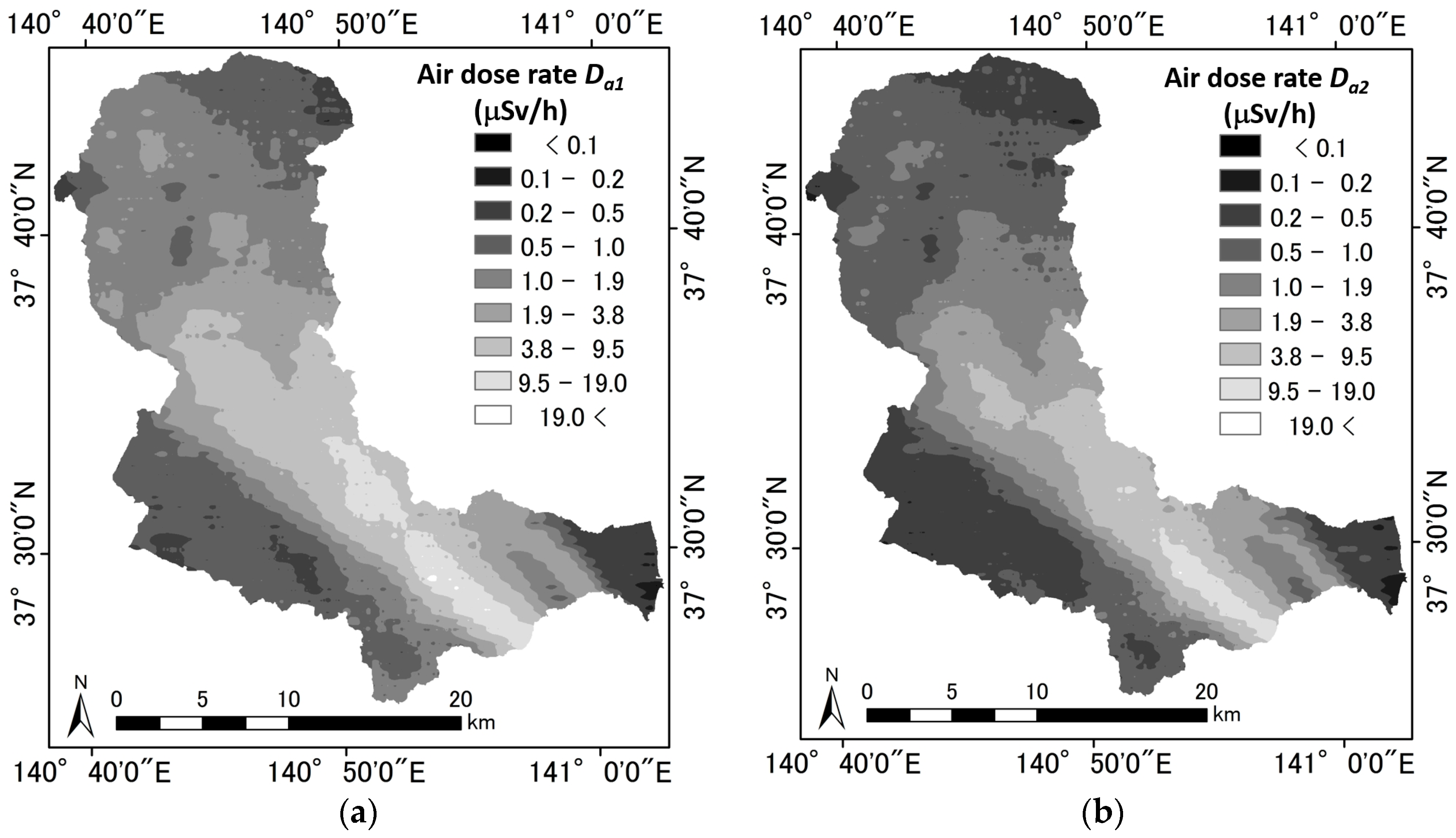
3.1. ARM Data before and after Snowfall

The dose rate maps before and after snowfall, as measured by ARM, are presented in Figure 4. The air dose rate in the northwestern area was relatively high. The air dose rates ranged from 0.1 to 20 μSv·h⁻¹. The ratio between the dose rate after snowfall, D_a2 (μSv·h⁻¹), and before snowfall, D_a1 (μSv·h⁻¹), is shown in Figure 5a. The D_a2/D_a1 ratio in the western area was higher than that in the eastern area. A large amount of snow falls in the western area because it is mountainous. Snow almost never falls in the eastern area because it is a flat coastal area.

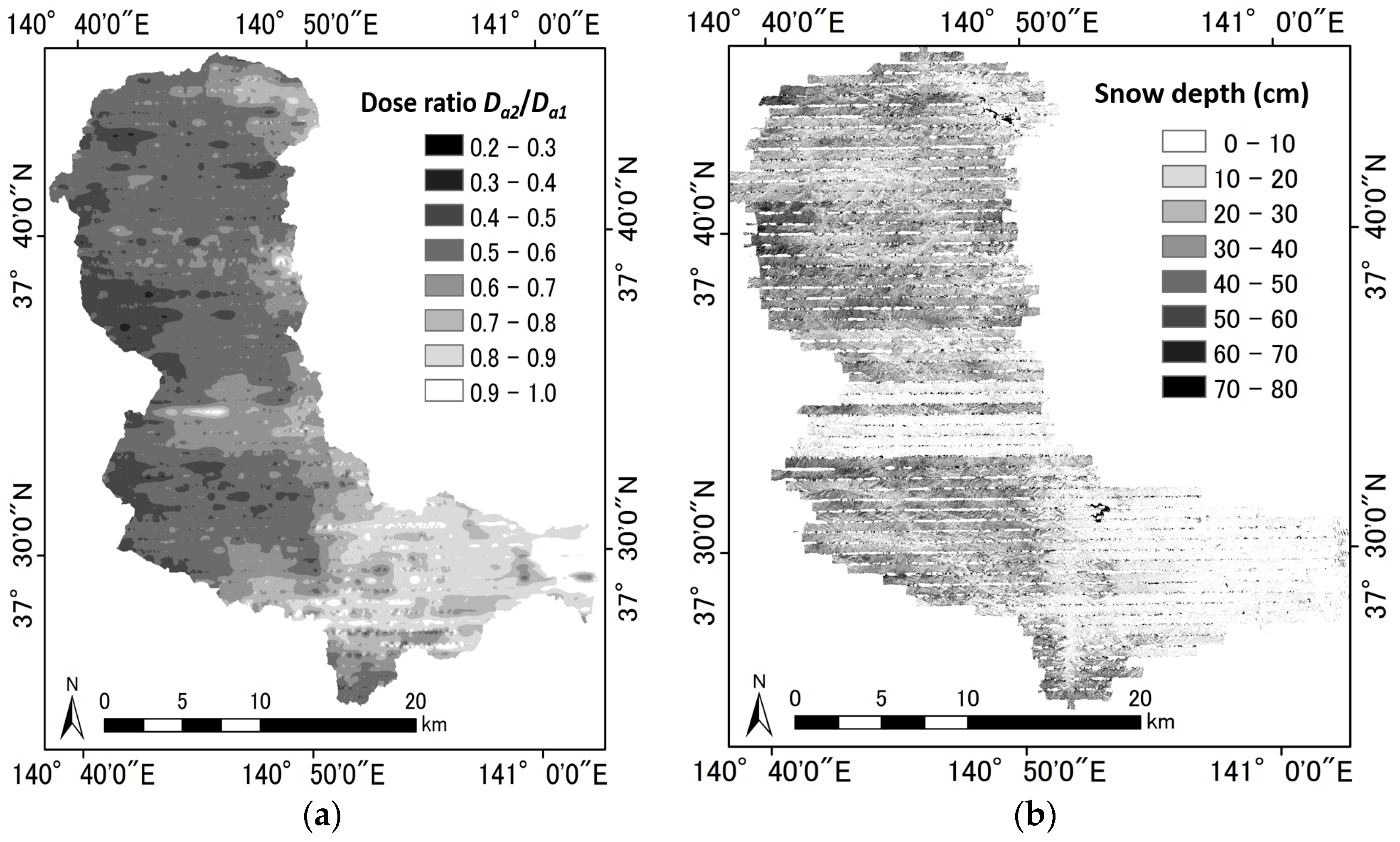
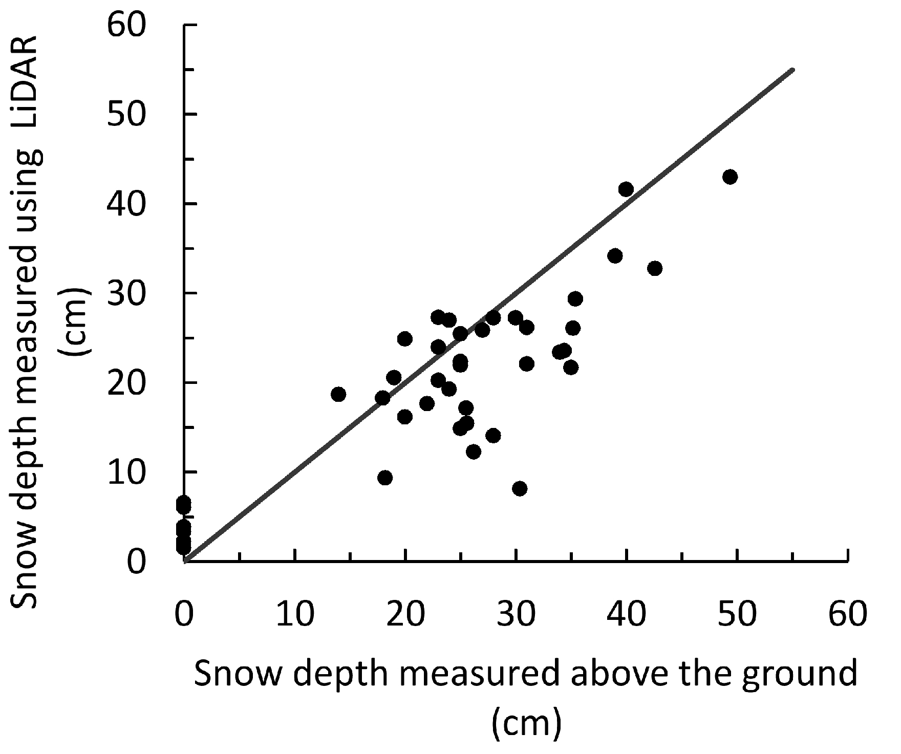
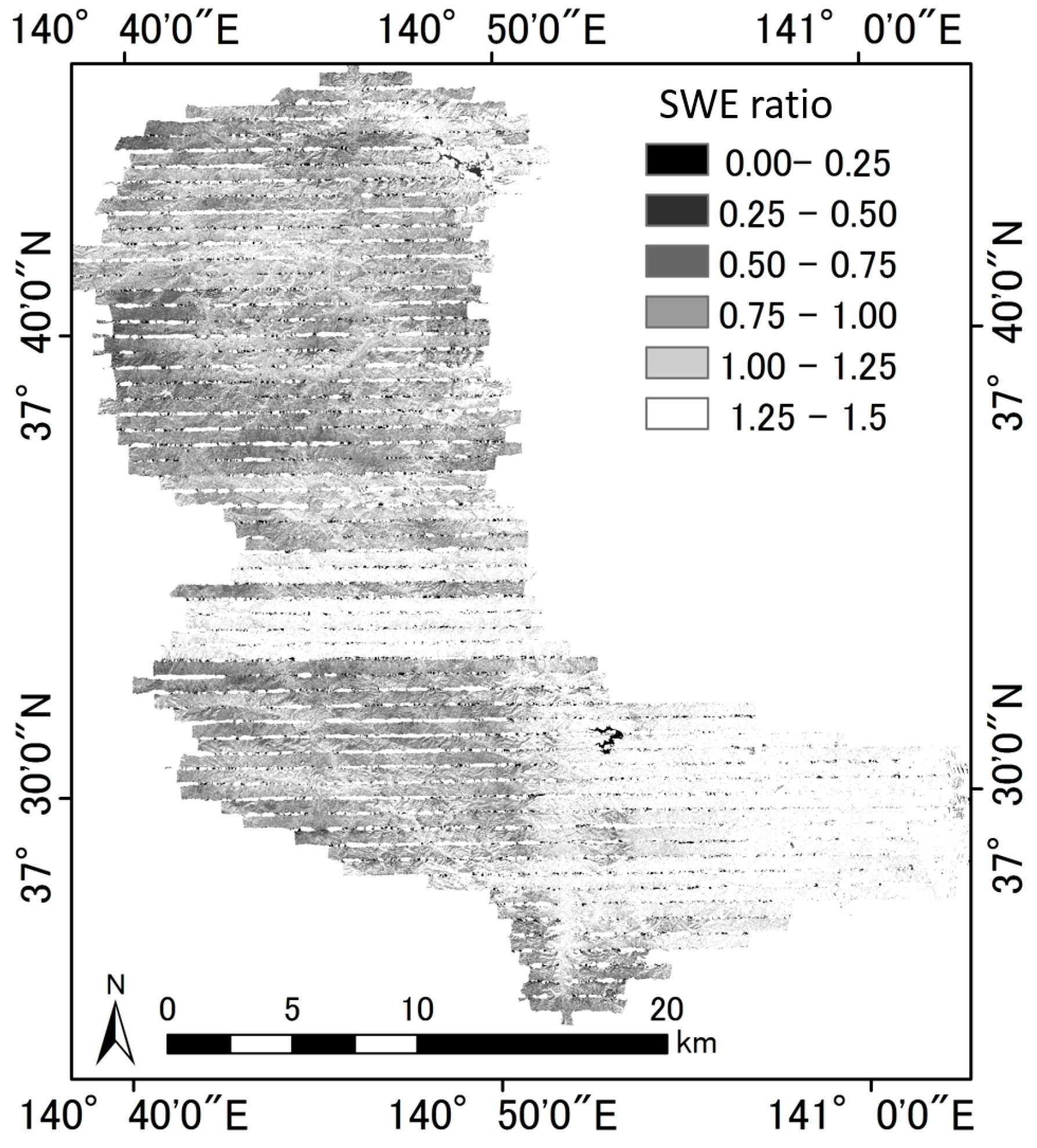
3.2. Snow Depth by LiDAR Data

The distribution map of snow depth determined from LiDAR data is shown in Figure 5b. The snow depth in the eastern region was lower than that in the western region. From Figure 5a,b, it was presented that the air dose rate decreased. A distribution map of the D_a2/D_a1 ratio appears to coincide with a map of the depth of the snow.

Some horizontal lines observed in Figure 5b appear to be caused by a lack of the overlap between the neighboring side edges of the scan area. Despite the 600 m interval between the ARM survey lines, the scan width in the direction of travel in LiDAR was less than 600 m. In addition, in the central region of Figure 5b, the snow depth decrease compared with the depth in the areas above and below the central region. This difference was caused by a difference in measurement dates.

Figure 6 compares the snow depths obtained by LiDAR with those obtained by ground measurements to confirm the validity of snow depths determined from LiDAR data. From Figure 6, it was shown that they have a positive correlation. Although the LiDAR measurement data tended to underestimate the ground measurement data, the snow depth determined from the LiDAR measurement data has enough precision to compare the radiation attenuation data by ARM.

4. Discussions

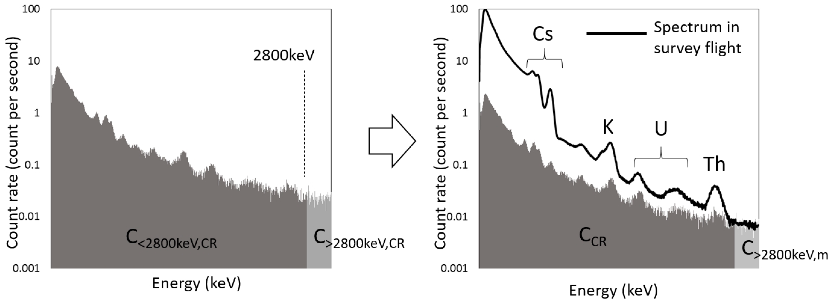
4.1. Correction Method of Snow Attenuation for ARM

The relation between D_a1 and D_a2 is shown in Figure 7a. The black circle indicates the average of D_a2. The error bars indicate the standard deviation of the air dose rate. The slope of the fitted curve was 0.78 and the D_a2 was underestimated in comparison with D_a1. This difference was caused by the attenuation of gamma rays by the snow layer. To correct this validity, the correction of the measured air dose rate after snowing was attempted. The shielding effect by snow layer are corrected with the following equation as

$$D^{\prime }=D/SF,$$

(4)

where D is the air dose rate measured using ARM after snowfall, D′ is the corrected air dose rate, and SF is the shielding factor of the snow layer. If SF can be estimated accurately, SF becomes equal to the D_a2/D_a1 ratio. Here, SF means the rate of the attenuation of gamma-ray flux due to the snow layer. Therefore, SF can be expressed as a function of the amount of snow, which is represented as SWE (g·cm⁻²). SWE is defined as the water weight per unit area and is converted from the amount of snow cover; it is obtained as

$$ESW=\rho \times t,$$

(5)

where ρ is snow density (g·cm⁻³) and t is snow depth (cm). The relation between the snow depth and the D_a2/D_a1 ratio is shown in Figure 8. The D_a2/D_a1 ratio was decreased with an increase in the snow depth up to the snow depth of 30 cm and gradually became constant over 30 cm. It is known that its trend is linked to snow density. The methods of density estimation were described in a following chapter.

In this correction method, the relation between SF and SWE have to be prepared. Then, to obtain this relation, we attempted simulation of the attenuation of gamma rays using the Monte Carlo calculation.

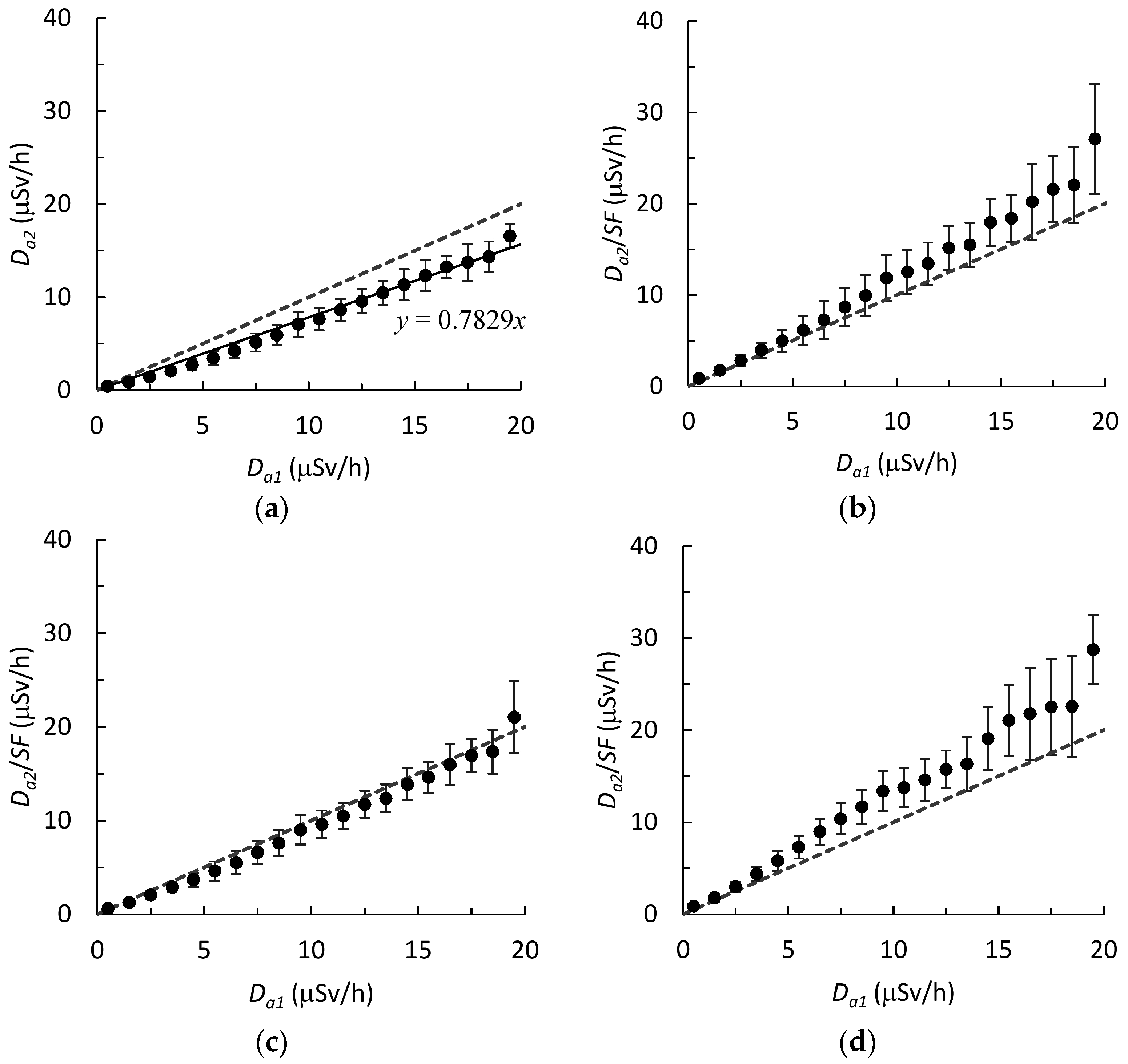
4.2. Simulation of Gamma Ray Attenuation with PHITS2

In the correction method described as Equation (4), the relation between an arbitrary SWE and gamma-ray attenuation by snow layer is essential. The gamma-ray flux in the case of snow cover with an arbitrary SWE was simulated using PHITS2, which is a Monte Carlo cord system used to simulate radiation transport [12]. In the gamma-ray flux calculation with PHITS2, the shape of the gamma-ray source is a flat plane with a radius of 500 m because almost one hundred percent of the total contribution of gamma rays from the ground originates from the area within a 500 m radius just below the ARM measurement point. Then, the snow cover is expressed as the water layer with uniform thickness of t, which is equal to SWE value and lies on the ground surface. The calculated result was shown in Figure 9. The relative flux decreased with increase in SWE.

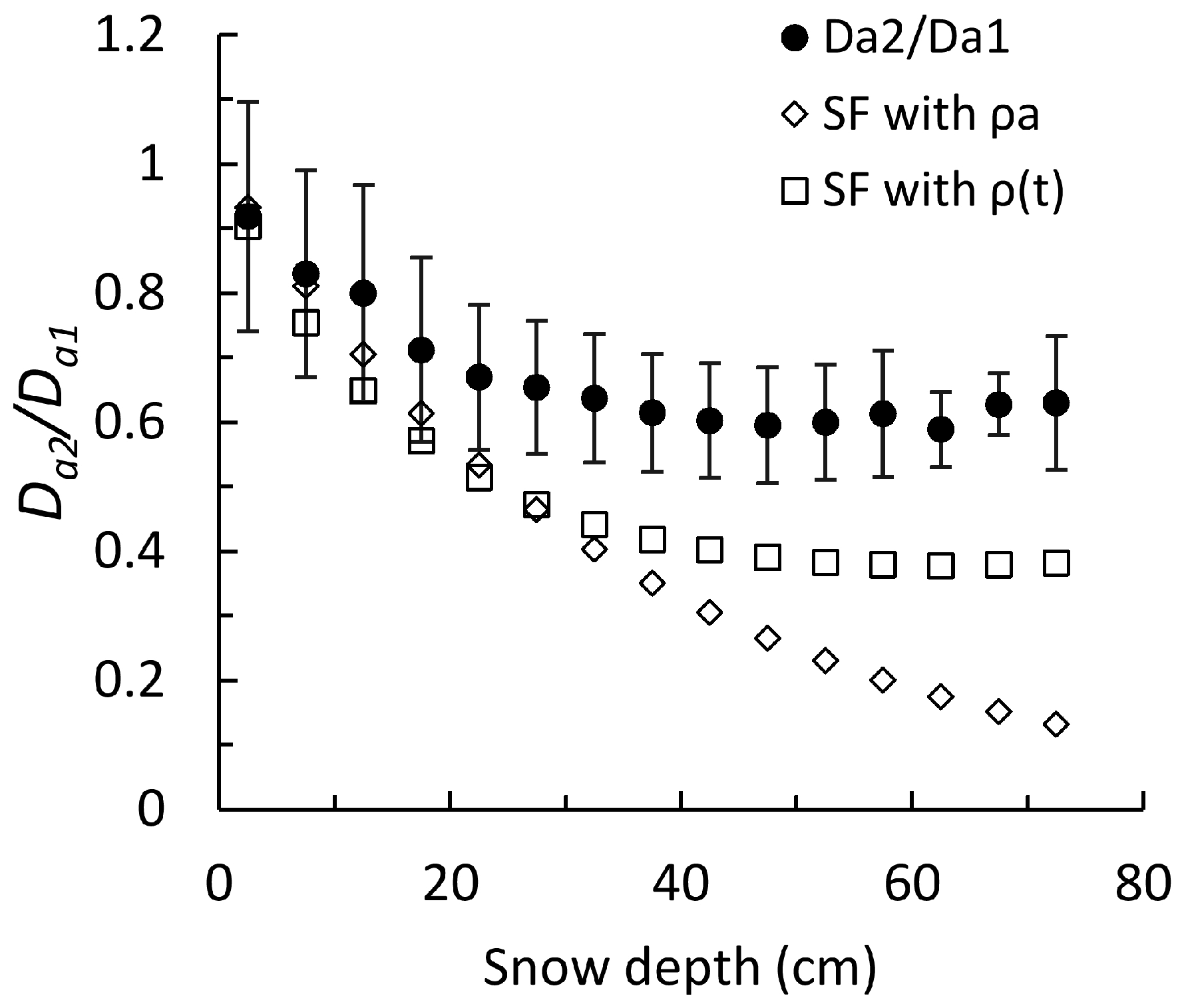
4.3. Correction Result of Attenuation by Snow Layer

Snow water equivalent is not able to measure by LiDAR. Then, we examined a method to estimate snow water equivalent with three approaches. The first is the method using the average snow density obtained from the ground measurement data and the snow depth obtained with LiDAR. The second is the method using the snow density obtained from the function of snow depth, which is defined on the basis of ground measurement data and the snow depth obtained with LiDAR. The third is the method using SWE obtained with the hydrological model. We evaluated validity of these methods by comparing the actual ARM data with corrected results using three types of methods.

4.3.1. Correction with an Average Snow Density

The method with an average snow density is simple and easy to apply. In this correction, snow depth obtained from LiDAR data and the average snow density, ρ_a, of 0.271 (g·cm⁻³) obtained from ground measurement results were used. To obtain the snow density, ρ, from ground measurement results, the snow volume, V, and the weight of snow, W, were measured above the ground by sampling snow packs. The measuring points were the same as the measuring points of the air dose rate shown in Figure 1 as black points. ρ was obtained as the following equation:

$$\rho =W/V.$$

(6)

The air dose rate was corrected using Equation (4), and the relation between D_a1 and the corrected air dose rate, D_a2/SF, is shown in Figure 7b. The corrected air dose rate was overestimated in comparison with the corresponding D_a1. In addition, the standard deviations increased. As for this cause, it is thought that snow density changes by depth. Figure 10 shows the relation between snow density and depth obtained from ground measurement results. Figure 10 shows that the snow density decreases with an increase in the snow depth. The relation between snow depth and SF obtained using PHITS2, and ρ_a is shown in as diamond shapes in Figure 8. In comparison with D_a2/D_a1, SF obtained using PHITS2 and ρ_a decreased rapidly with increase in the snow depth as shown in Figure 8. This rapid decrease caused the extra correction. Then, it resulted in the overestimation of the air dose rate. Therefore, the choice of snow density used in the calculation of SF is important. Using an appropriate value might result in an improvement of the correction accuracy and a decrease in the standard deviations. However, in the case of a wide range of snow depth in a survey area, there is a potential for an increase of the effects by the constant snow density on the correction accuracy.

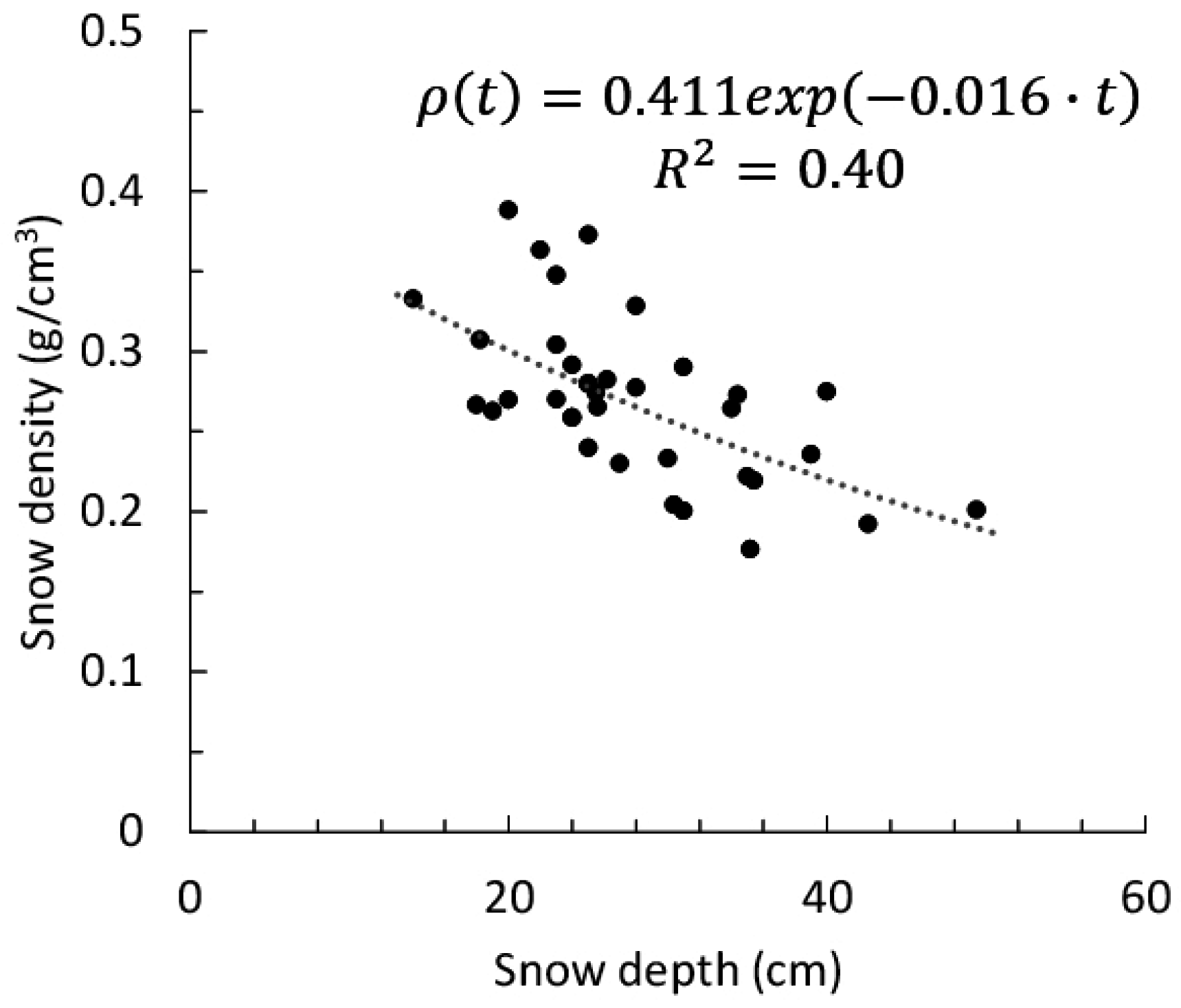
4.3.2. Correction with Density as a Function of Snow Depth

In the previous Section 4.3.1, the snow density decreased with increasing of the snow depth. Therefore, we also attempted to correct the air dose rate with PHITS2 and the snow density, ρ(t), which varies with the snow depth, as shown in Figure 10. Function ρ(t) was obtained as the fitted curve of the measurement results as shown in Figure 10. The map of the ratio of SWE obtained using ρ(t) to SWE obtained using ρ_a was shown by Figure 11. This value of SWE ratio was an index of difference of snow density. Compared with Figure 5b, the ratio was tended to decrease with increasing of the snow depth. The corrected result of the air dose rate is shown in Figure 7c. In comparison with the result obtained using ρ_a, which is shown in Figure 7b, the relation between D_a1 and D_a2/SF became closer to the line y = x line and the standard deviation became smaller. The corrected SF is shown in Figure 8 as squares. The trend of the SF obtained using ρ(t) appears to be more similar to the SF obtained from measured D_a1 and D_a2 than the trend of the SF obtained using ρ_a. Thus, the correction accuracy was improved through the use of ρ(t). However, compared with the standard deviation of D_a2 (Figure 7a), the standard deviation of the corrected air dose rate (Figure 7c) increased. This result suggests that the snow density varies not only with the snow thickness but also with local conditions such as temperature, elevation, and land use. Therefore, more accurate estimates of the local snow density are needed.

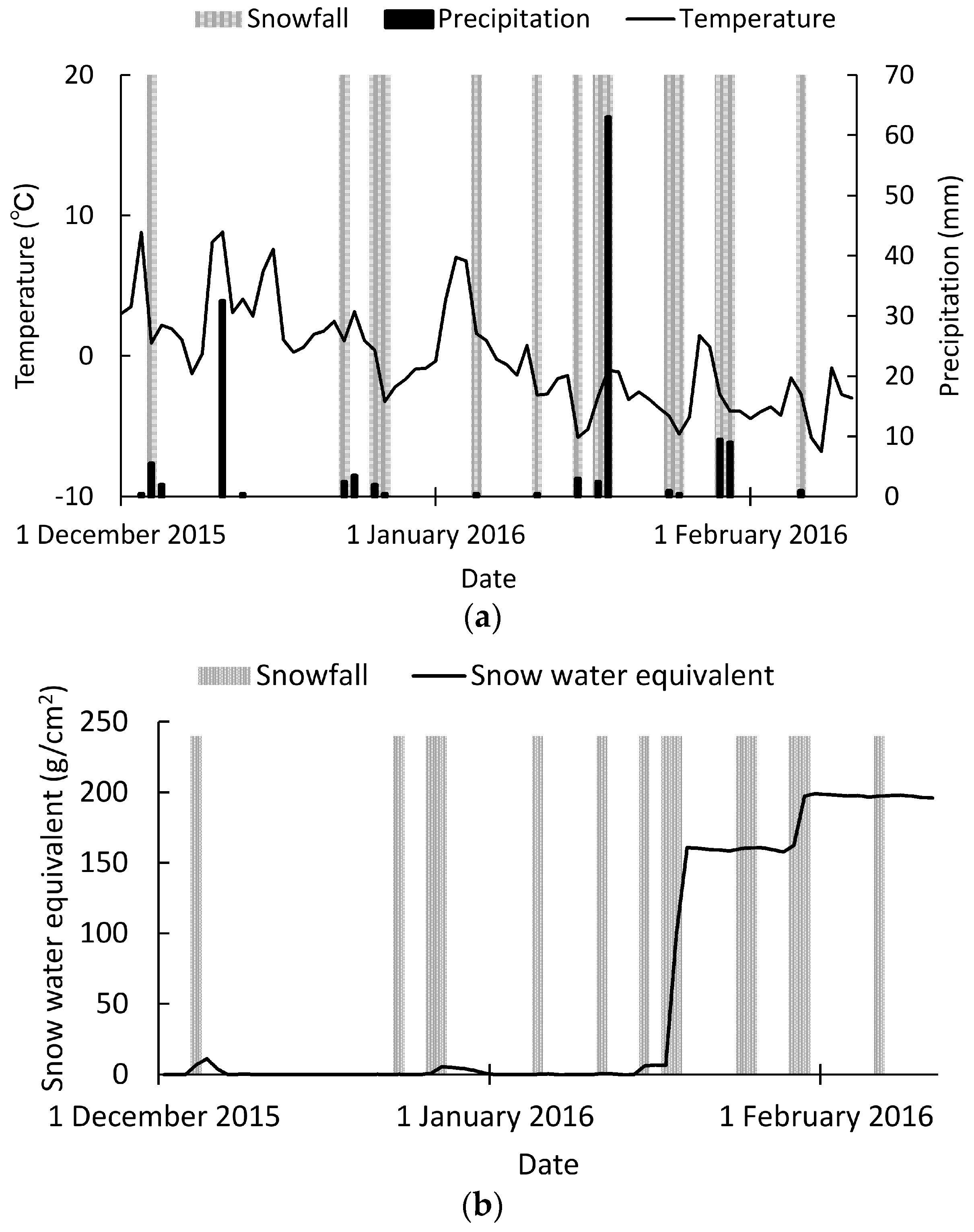
4.3.3. Correction with the Hydrological Model

The method with the hydrological model is the method with only calculation and does not need snow depth measurement. The hydrological model can represent snow conditions under the several meteorological conditions. By using the hydrological model, the process of the snow accumulating, melting and runoff can be estimated. The hydrological model was developed to model different aspects of water cycles including snow [13,14]. In the calculation with the hydrological mode, the meteorological data was required. The meteorological data was obtained from Automated Meteorological Data Acquisition System (AMeDAS) [15]. We obtained the information of precipitation, temperatures, amount of sunlight and elevations from 1 December 2015 to 11 February 2016.

The SWE at the ARM measurement positions was calculated with the hydrological model. The details of the calculation process and parameters are the same as the present Japanese research articles shown in [14]. The daily meteorological trends used in the calculations were shown in Figure 12a, and the example of calculated results of SWE at the point of P₁ was shown in Figure 12b. The point of P₁ is the point with the highest elevation among the ground measurement points shown in Figure 1. From this result, SF at each position was calculated. The corrected result of D_a2 was shown in Figure 7d. Compared with other results shown in Figure 7, the D_a2/SF was overestimated, and the standard deviation became the largest. It could be expected that the snow water equivalent can be obtained to a certain precision by using the hydrological model, though more improvement of the calculation precision is necessary.

5. Conclusions

To correct ARM data for gamma-ray attenuation due to snow layers, the measurement of snow depth with LiDAR was performed. On the whole, snow depth determined by LiDAR was shallower than that determined by ground measurements. Using snow depth obtained from LiDAR data, we collected for gamma-ray attenuation using two estimates of snow density: ρ_a and ρ(t). In the case of attenuation correction with ρ(t), the underestimation of the air dose rate was improved. In addition, comparing the correction results with each density estimate clarified that the density of the snow layer is one of the most important factors in the correction. Because the extent of gamma-ray attenuation is presumably proportional to the SWE, the density of the snow layer should be obtained as accurately as possible. If the accurate local density of the snow layer can be obtained, the correction accuracy achieved using PHITS2 is comparable with that achieved using measurement data. In this study, the snow layer density was determined using ground measurement. However, in the case where survey is required over a broader area, ground measurements have limitations. SWE has been reported to change with changes in meteorological conditions and elevations [14,16]. Then, in addition, we attempt to correct the air dose rate with SWE obtained with the hydrological model. However, the correction accuracy was not improved. In future work, we will obtain SWE estimated using data from not only the AMeDAS, but also the Earth Observing System (EOS) [17], which will enable improvement of the accuracy of the correction.

References

1. Sanada, Y.; Sugita, T.; Nishizawa, Y.; Kondo, A.; Torii, T. The aerial radiation monitoring in Japan after the Fukushima Dai-ichi nuclear power plant accident. Prog. Nucl. Sci. Technol. 2014, 4, 76–80. [Google Scholar] [CrossRef]
2. Lyons, C.; Colton, D. Aerial measurement system in Japan. Health Phys. 2012, 102, 482–484. [Google Scholar] [CrossRef] [PubMed]
3. US, Japan Develop a New Method for Radiological Dose Assessment in Area Surrounding Fukushima Daiichi Nuclear Power Plants. Available online: https://nnsa.energy.gov/mediaroom/pressreleases/nnsajaea062713 (accessed on 26 September 2016).
4. Sanada, Y.; Mori, A.; Ishizaki, A.; Munakata, M.; Nakayama, S.; Nishizawa, Y.; Urabe, Y.; Nakanishi, C. Radiation monitoring using manned helicopter around the Fukushima Nuclear Power Station in the fiscal year 2014. JAEA Res. 2015. (In Japanese) [Google Scholar] [CrossRef]
5. International Atomic Energy Agency (IAEA). Guidelines for Radioelement Mapping Using Gamma Ray Spectrometry Data; IAEA: Vienna, Austria, 2003. [Google Scholar]
6. Bergstrom, S.; Brandt, M. Snow mapping and hydrological forecasting by airborne γ-ray spectrometry in Northern Sweden. In Proceedings of the Tsunami Symposium, Hamburg, Germany, 15–16 August 1983; pp. 421–427.
7. ENDRESTØL, G.O. Principle and method for measurement of snow water equivalent by detection of natural gamma radiation. Hydrol. Sci. Bull. 1980, 25, 77–83. [Google Scholar] [CrossRef]
8. Nagaoka, T.; Sakamoto, R.; Saito, K.; Tsutsumi, M.; Moriuchi, S. Diminution of Terrestrial gamma ray exposure rate due to snow cover. Jpn. J. Health Phys. 1988, 23, 309–315. (In Japanese) [Google Scholar] [CrossRef]
9. Latifi, H.; Heurich, M.; Hartig, F.; Müller, J.; Krzystek, P.; Jehl, H.; Dech, S. Estimating over- and understorey canopy density of temperate mixed stands by airborne LiDAR data. Forestry 2016, 89, 69–81. [Google Scholar] [CrossRef]
10. Li, Z.; Guo, X. Remote sensing of terrestrial non-photosynthetic vegetation using hyperspectral, multispectral, SAR, and LiDAR data. Prog. Phys. Geogr. 2016, 40, 276–304. [Google Scholar] [CrossRef]
11. Liu, X. Airborne LiDAR for DEM generation: some critical issues. Prog. Phys. Geogr. 2008, 32, 31–49. [Google Scholar]
12. Sato, T.; Niita, K.; Matsuda, N.; Hashimoto, S.; Iwamoto, Y.; Noda, S.; Ogawa, T.; Iwase, H.; Nakashima, H.; Fukahori, T.; et al. Particle and heavy ion transport code system, PHITS, version 2.52. J. Nucl. Sci. Technol. 2013, 50, 913–923. [Google Scholar] [CrossRef]
13. Davison, B. Snow Accumulation in a Distributed Hydrological Model. Master’s Degree, University of Waterloo, Waterloo, ON, Canada, 2004. [Google Scholar]
14. Suizu, S. A snowmelt and water equivalent snow model applicable to an extensive area. J. Jpn. Soc. Snow Ice 2002, 64, 617–630. (In Japanese) [Google Scholar] [CrossRef]
15. Japan Meteorological Agency. Temperature. Available online: http://www.jma.go.jp/en/amedas/ (accessed on 1 June 2016).
16. Ohta, T. A distributed snowmelt prediction model in mountain areas based on an energy balance method. Ann. Glaciol. 1994, 19, 107–113. [Google Scholar]
17. NASA’s Earth Observing System. Available online: http://eospso.nasa.gov/ (accessed on 1 June 2016).
Figure 1. Scheme of survey area and measurement points. Black dots indicate ground measurement points. Straight lines indicate survey lines of airborne radiation survey (ARM). P1 indicates the ground measurement point with the highest elevation.
Remotesensing 08 00892 g001
Figure 2. Conceptual schema of the geometrical difference between ARM and ground measurement.
Remotesensing 08 00892 g002
Figure 3. Images of subtracting background caused by cosmic rays.
Remotesensing 08 00892 g003
Figure 4. Maps of the air dose rate: (a) before snowfall; and (b) after snowfall.
Remotesensing 08 00892 g004
Figure 5. (a) Distribution of the ratio between the air dose rate before and after snowfall (SF); and (b) distribution of snow depth.
Remotesensing 08 00892 g005
Figure 6. Relation between snow depth obtained by ground measurement and that obtained by LiDAR. The solid line indicates the y = x line.
Remotesensing 08 00892 g006
Figure 7. Relation between air dose rates before and after snowfall (a) without correction; (b) with correction using SF from results in PHITS2 and ρa; (c) with correction using SF from results in PHITS2 and ρ(t); and (d) with correction using the hydrological model. Dashed lines in each figure indicate the y = x line. The solid line in (a) indicates the fitted curve.
Remotesensing 08 00892 g007
Figure 8. Relation between snow depth and the average ratio of the air dose rate after snowfall to that before snowfall in the ARM and SF obtained using two approaches.
Remotesensing 08 00892 g008
Figure 9. Relation between snow water equivalent and relative flux 300 m up calculated with PHITS2.
Remotesensing 08 00892 g009
Figure 10. Relation between measured snow depth and density.
Remotesensing 08 00892 g010
Figure 11. Distribution of the ratio between SWE obtained using ρ(t) and SWE obtained using ρa.
Remotesensing 08 00892 g011
Figure 12. (a) Trend of temperature and precipitation at the closest observation points to the survey area; and (b) trend of the calculated snow water equivalent with the hydrological model at the point of P1 that is shown in Figure 1.
Remotesensing 08 00892 g012