
Lake Level Estimation Based on CryoSat-2 SAR Altimetry and Multi-Looked Waveform Classification


Abstract
:
1. Introduction
2. Study Area
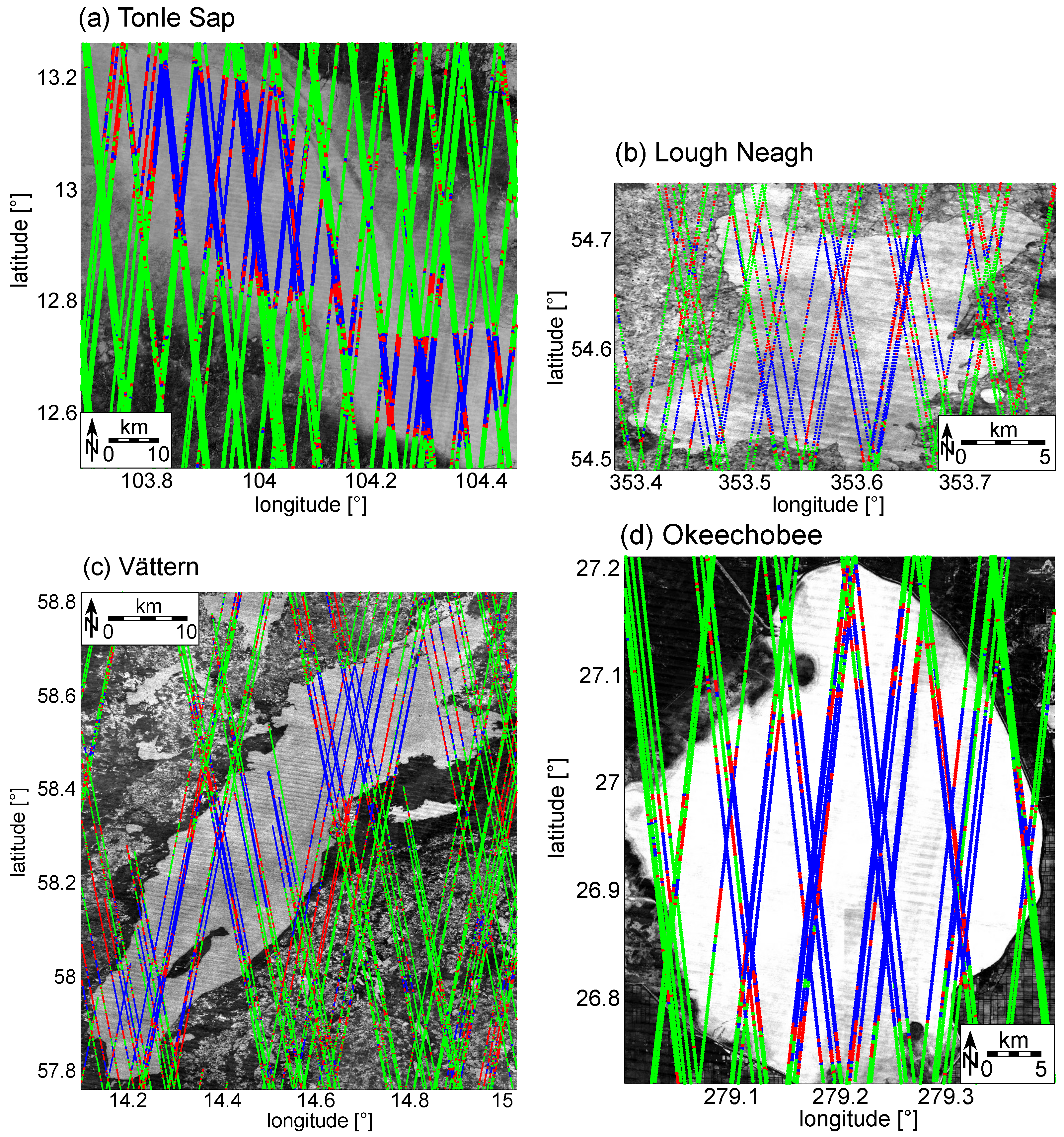
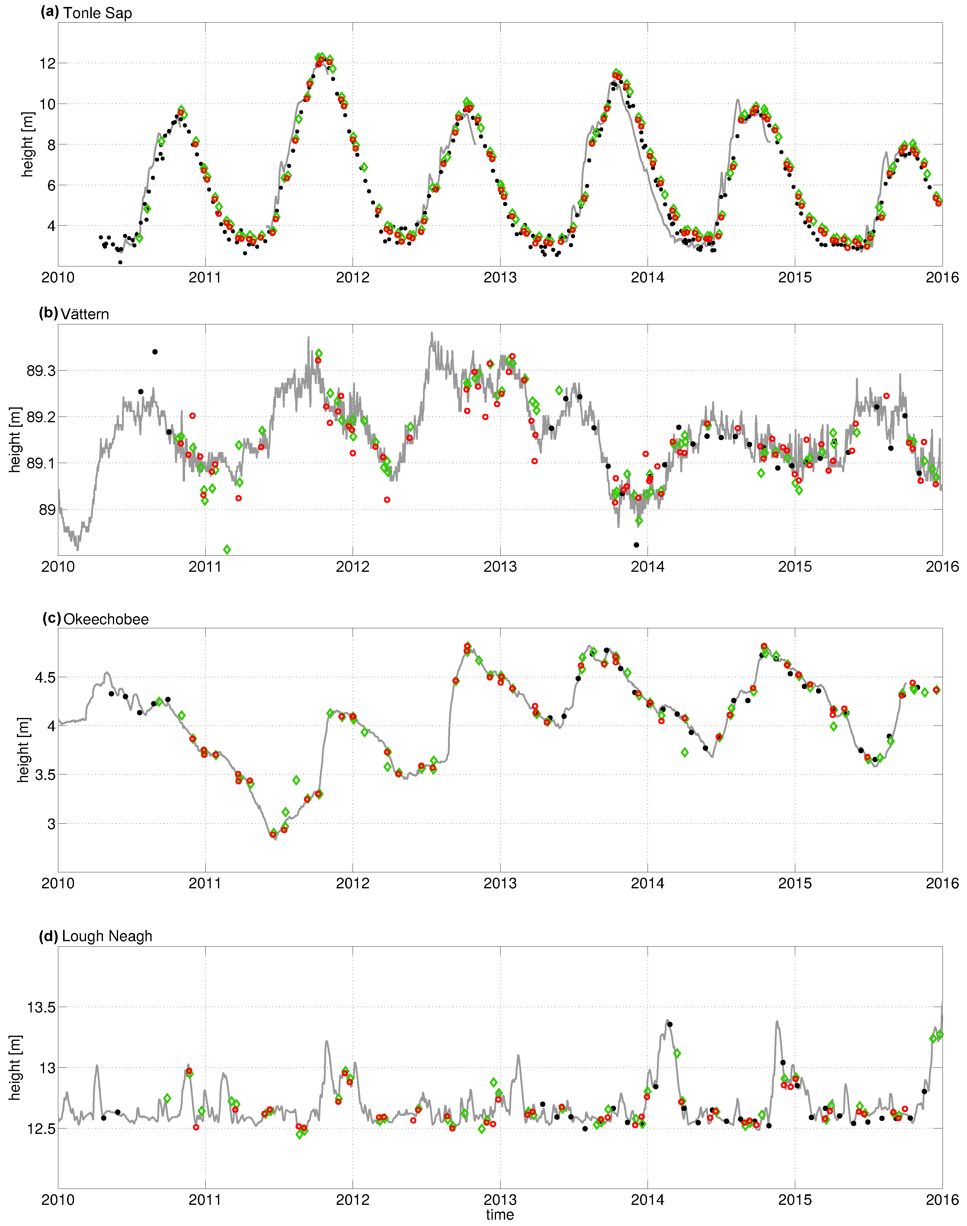
- Tonle Sap is the largest lake in Southeast Asia with a surface area of about 2600 km during the dry season and 10,400 km during the flood season. Accordingly, the water level of the lake shows a strong annual signal which varies between 2.3 m and 12.4 m. The surrounding landscape of the lake is flat and contains a great deal of rivers and wetland areas especially during the flood season.
- Vättern is the second largest lake in Sweden with a surface area of about 1912 km. It does not show a significant annual signal and the water level of the lake shows only variations of about 1 m. The landscape around the lake is flat with three small lakes around the lake Vättern.
- Okeechobee is the largest lake in Florida with a surface area of about 1900 km. The water level of the lake varies between 2.6 m and 5.4 m with no significant annual signal. The lake is located in a flat territory and it is mainly surrounded by wetlands.
- Lough Neagh is the largest lake of the island Ireland with a surface area of about 392 km. The water level of the lake shows an annual signal and varies between 12.2 m and 13.3 m. The lake is situated in lowland with a few smaller lakes around Lough Neagh.
3. Data Sources
3.1. CryoSat-2 L1b Product: SAR Mode
3.2. In-Situ Gauging Data
- The Mekong River Commission (http://ffw.mrcmekong.org/) maintains the gauging station Prek Kdam which is not located directly at the Lake Tonle Sap but next to the Lake Tonle Sap at the Prek Kdam Bridge crossing the Tonle Sap River. Therefore, these gauging data represent the water level of the Lake Tonle Sap quite well. Unfortunately, since 2009 the water level time series are only provided during the flood season from June to October but not for the dry season from November to May. The water level time series are referred to the zero gauge which is 0.08 m above the mean sea level.
- The Swedish Meteorological and Hydrological Institute (http://vattenwebb.smhi.se/station/) offers gauging data for the Lake Vättern with respect to the Swedish height system “Rikets höjdsystem 1900” (RH 00). The gauging station for the Lake Vättern is located in the city Motala along the river Motala ström.
- The National Water Information System (http://waterdata.usgs.gov/nwis/sw) provides gauging data for the Lake Okeechobee regarding to the National Geodetic Vertical Datum of 1929 (NGVD 29). The daily water levels are averages of the measurements of the 14 gauging stations located at the Lake Okeechobee.
- The Rivers Agency, Department of Agriculture and Rural Development (https://www.dardni.gov.uk/rivers-agency) holds gauging data for the Lake Lough Neagh with respect to the height system metres ordance datum Belfast (mOD Belfast). While for the time span 2002–2008 the data of two gauging stations on the Lake Lough Neagh are averaged, for the time span 2008–2016 the data of four gauging stations on the Lake Lough Neagh are averaged.
3.3. DAHITI: Water Level Time Series from Multi-Mission Satellite Altimetry
3.4. AltWater: Modeled Water Level Time Series From CryoSat-2
4. Method
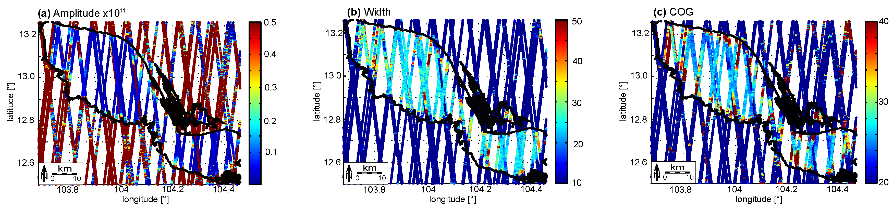
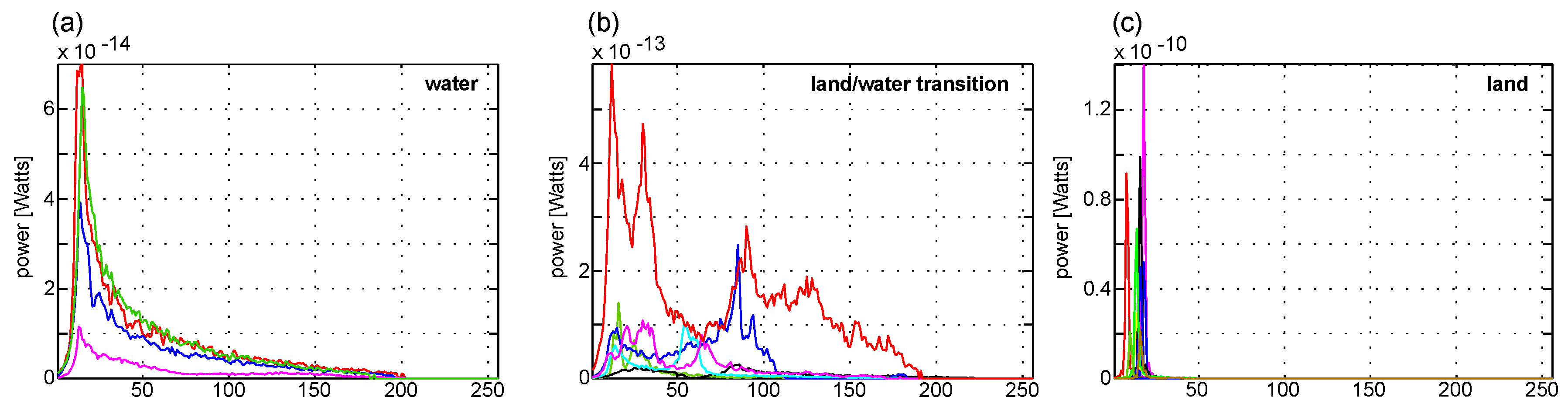
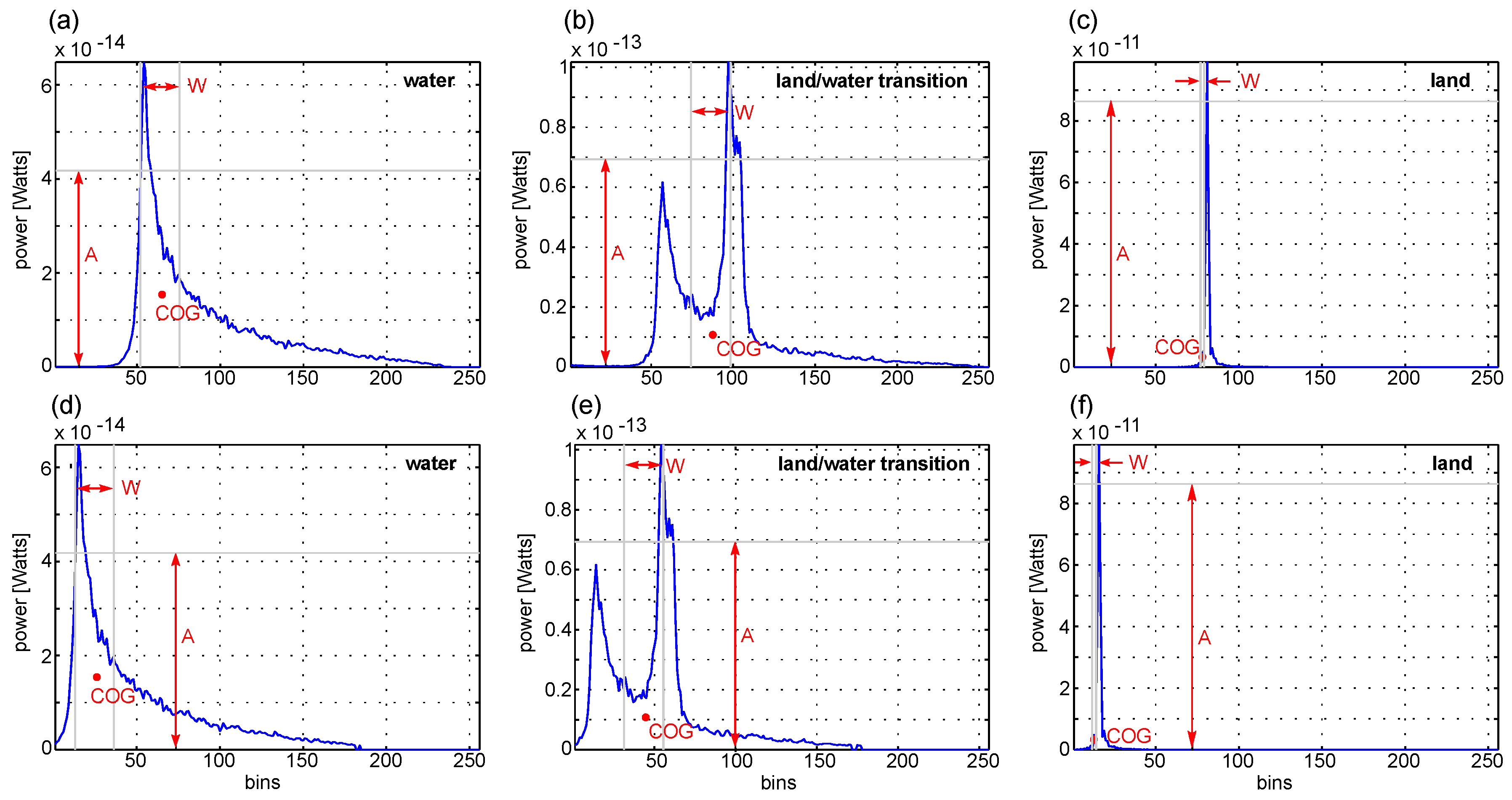
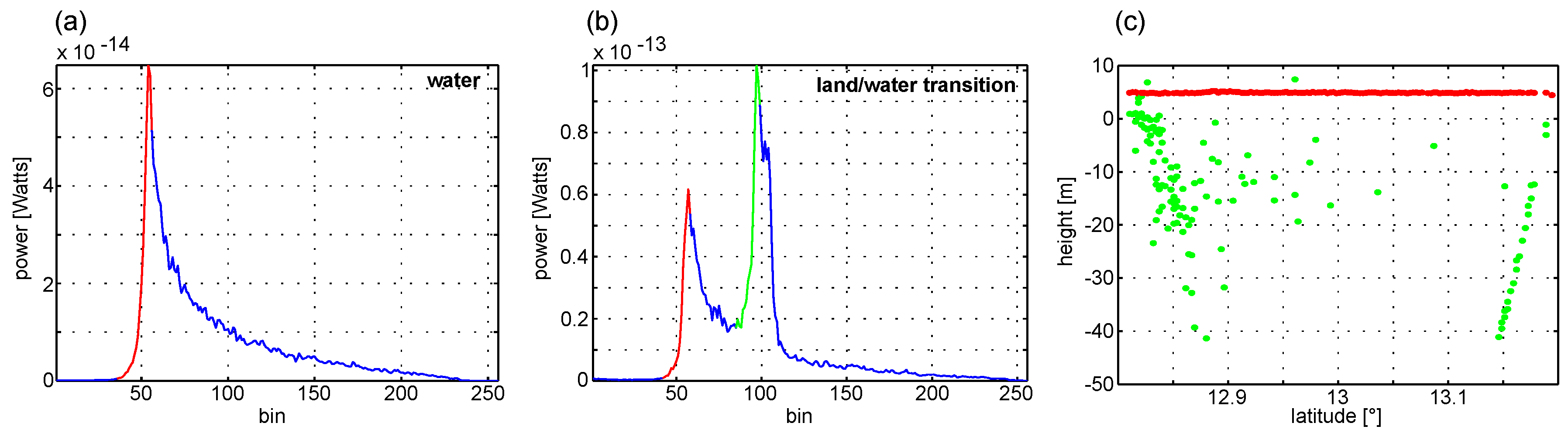
4.1. Waveform Classification
4.2. Waveform Retracking Algorithm
4.3. Outlier Rejection
5. Results, Validation and Discussion
6. Conclusions
Acknowledgments
Author Contributions
Conflicts of Interest
References
- Fekete, B.M.; Vorosmarty, C.J. The current status of global river discharge monitoring and potential new technologies complementing traditional discharge measurements. IAHS Publ. 2007, 309, 129–136. [Google Scholar]
- Birkett, C.M. Radar altimetry: A new concept in monitoring lake level changes. Eos Trans. Am. Geophys. Union 1994, 75, 273–275. [Google Scholar] [CrossRef]
- Crétaux, J.F.; Birkett, C. Lake studies from satellite radar altimetry. C. R. Geosci. 2006, 338, 1098–1112. [Google Scholar] [CrossRef]
- Crétaux, J.F.; Jelinski, W.; Calmant, S.; Kouraev, A.; Vuglinski, V.; Bergé-Nguyen, M.; Gennero, M.C.; Nino, F.; Rio, R.A.D.; Cazenave, A.; et al. SOLOS: A lake database to monitor in the Near Real Time water level and storage variations from remote sensing data. Adv. Space Res. 2011, 47, 1497–1507. [Google Scholar] [CrossRef]
- Schwatke, C.; Dettmering, D.; Boergens, E.; Bosch, W. Potential of SARAL/AltiKa for inland water applications. Mar. Geod. 2015, 38, 626–643. [Google Scholar] [CrossRef]
- Nielsen, K.; Stensen, L.; Andersen, O.B.; Villadsen, H.; Knudsen, P. Validation of CryoSat-2 SAR mode based lake levels. Remote Sens. Environ. 2015, 171, 162–170. [Google Scholar] [CrossRef] [Green Version]
- Villadsen, H.; Deng, X.; Andersen, O.B.; Stensen, L.; Nielsen, K.; Knudsen, P. Improved inland water levels from SAR altimetry using novel empirical and physical retrackers. J. Hydrol. 2016, 537, 234–247. [Google Scholar] [CrossRef] [Green Version]
- Yang, L.; Lin, M.; Liu, Q.; Pan, D. A coastal altimetry retracking strategy based on waveform classification and sub-waveform extraction. Int. J. Remote Sens. 2012, 33, 7806–7819. [Google Scholar] [CrossRef]
- Zygmuntowska, M.; Khvorostovsky, K.; Helm, V.; Sandven, S. Waveform classification on airborne synthetic aperture radar altimeter over Arctic sea ice. Cryosphere 2013, 7, 1315–1324. [Google Scholar] [CrossRef]
- Desai, S.; Chander, S.; Ganguly, D.; Chauhan, P.; Lele, P.D.; James, M.E. Waveform Classification and Water-Land Transition over the Brahmaputra River using SARAL/AltiKa & Jason-2 Altimeter. Indian Soc. Remote Sens. 2015, 43, 475–485. [Google Scholar]
- Gommenginger, C.; Thibaut, P.; Fenoglio-Marc, L.; Quartly, G.; Deng, X.; Gómez-Enri, J.; Challenor, P.; Gau, Y. Retracking altimeter waveforms near the coast. In Coastal Altimetry; Benveniste, J., Cipollini, P., Kostianoy, A.G., Vignudelli, S., Eds.; Springer: Berlin, Germany, 2011; pp. 61–101. [Google Scholar]
- Raney, R.K. The Delay/Doppler Radar Altimeter. IEEE Trans. Geosci. Remote Sens. 1998, 36, 1578–1588. [Google Scholar] [CrossRef]
- Bouzinac, C. CryoSat Product Handbook. Available online: https://earth.esa.int/documents/10174/125272/CryoSat_Product_Handbook (accessed on 1 April 2012).
- Pavlis, N.K.; Holmes, S.A.; Kenyon, S.C.; Factor, J.K. The development and evaluation of the Earth Gravitational Model 2008 (EGM2008). J. Geophys. Res. 2012, 117. [Google Scholar] [CrossRef]
- Iijima, B.A.; Harris, I.L.; Ho, C.M.; Lindqwister, U.J.; Mannucci, A.J.; Pi, X.; Reyes, M.J.; Sparks, L.C.; Wilson, B.D. Automated daily process for global ionospheric total electron content maps and satellite ocean altimeter ionospheric calibration based on Global Positioning System data. J. Atmos. Sol. Terr. Phys. 1999, 61, 1205–1218. [Google Scholar] [CrossRef]
- Boehm, J.; Kouba, J. Forecast Vienna Mapping Functions 1 for real-time analysis of space geodetic observations. J. Geod. 2009, 83, 397–401. [Google Scholar] [CrossRef]
- Förste, C.; Bruinsma, S.; Flechtner, F.; Marty, J.; Lemoine, J.; Dahle, C.; Abrikosov, O.; Neumayer, H.; Biancale, R.; Barthelmes, F.; et al. A new release of EIGEN-6: The latest combined global gravity field model including LAGEOS, GRACE and GOCE data from the collaboration of GFZ Potsdam and GRGS Toulouse. In Proceedings of the 2012 EGU General Assembly, Vienna, Austria, 22–27 April 2012.
- Schwatke, C.; Dettmering, D.; Bosch, W.; Seitz, F. DAHITI—An innovative approach for estimating water level time series over inland waters using multi-mission satellite altimetry. Hydrol. Earth Syst. Sci. 2015, 19, 4345–4364. [Google Scholar] [CrossRef]
- Smola, A.J.; Schölkopf, B. A tutorial on support vector regression. Stat. Comput. 2004, 14, 199–222. [Google Scholar] [CrossRef]
- Bosch, W.; Dettmering, D.; Schwatke, C. Multi-mission cross-calibration of satellite altimeters: Constructing a long-term data record for global and regional sea level change studies. Remote Sens. 2014, 6, 2255–2281. [Google Scholar] [CrossRef]
- Jain, M.; Andersen, O.B.; Dall, J.; Stenseng, I. Sea surface height determination in the Arctic using CryoSat-2 SAR data from primary peak empirical retrackers. Adv. Space Res. 2015, 55, 40–50. [Google Scholar] [CrossRef]
- Wingham, D.J.; Raplex, C.G.; Griffiths, H. New techniques in satellite altimeter tracking systems. In Proceedings of IGARSS 86 Symposium; ESA Publications Division: Noordwijk, The Netherlands, 1986; pp. 1339–1344. [Google Scholar]
- MacQueen, J. Some methods for classification and analysis of multivariate observations. In Proceedings of the Fifth Berkeley Symposium on Mathematical Statistics and Probability: Statistics; Le Cam, L.M., Neyman, J., Eds.; University of California Press: Berkeley, CA, USA, 1967; Volume 1, pp. 281–297. [Google Scholar]
- Singh, A.; Yadav, A.; Rana, A. K-means with Three different Distance Metrics. Int. J. Comp. Appl. 2013, 67, 13–17. [Google Scholar] [CrossRef]
- Timm, N.H. Cluster Analysis and Multidimensional Scaling. In Applied Multivariate Analysis; Casella, G., Fienberg, S., Olkin, I., Eds.; Springer Texts in Statistics: New York, NY, USA, 2002; pp. 515–555. [Google Scholar]
- Xu, R.; Wunsch, D.C. Partitional Clustering. In Clustering; Hanzo, L., Ed.; John Wiley & Sons: Hoboken, NJ, USA, 2009; pp. 63–110. [Google Scholar]


| Correction | Source/Model | Reference |
|---|---|---|
| Ionosphere | Jet Propulsion Laboratory-Global Ionosphere Maps (JPL-GIM), International Reference Ionosphere (IRI) scaled | [15] |
| Wet troposphere | ECMWF () for Vienna Mapping Functions 1 (VMF1) | [16] |
| Dry troposphere | ECMWF () for Vienna Mapping Functions 1 (VMF1) | [16] |
| Solid Earth tide | CryoSat-2 Level 1b | [13] |
| Pole tide | CryoSat-2 Level 1b | [13] |
| Lake | Size | Tracks | DGFI-TUM | DTU | DAHITI | ||||||
|---|---|---|---|---|---|---|---|---|---|---|---|
| RMS | No. | RMS | No. | RMS | No. | ||||||
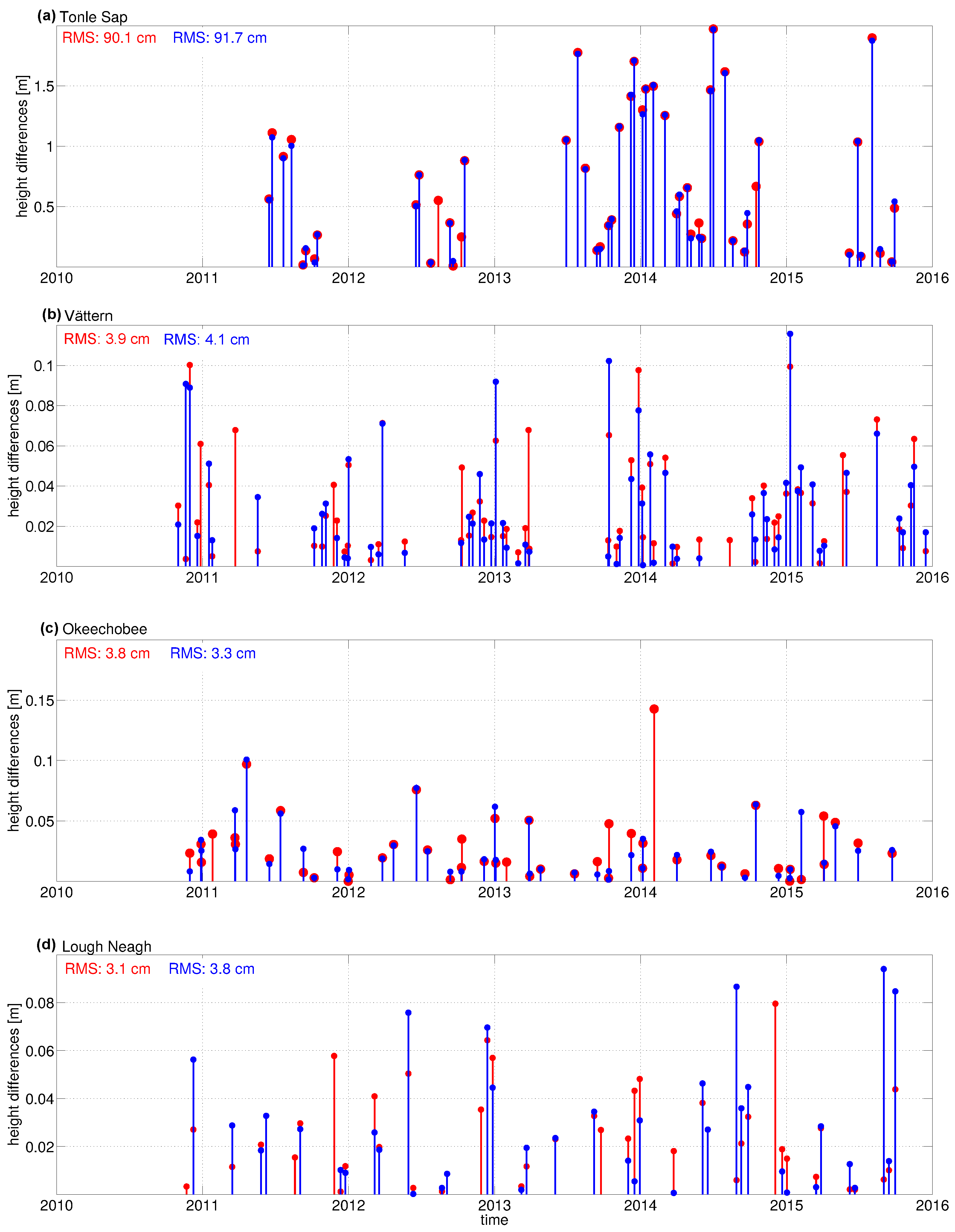
| Tonle Sap | 2600 | 107 | 90.1 | 0.90 | 107 | 96.1 | 0.87 | 137 | 72.4 | 0.93 | 233 |
| Vättern | 1912 | 76 | 3.9 | 0.79 | 71 | 4.6 | 0.75 | 71 | 4.0 | 0.73 | 29 |
| Okeechobee | 1900 | 54 | 3.8 | 0.99 | 52 | 7.3 | 0.98 | 73 | 4.9 | 0.97 | 33 |
| Neagh | 392 | 54 | 3.1 | 0.95 | 43 | 6.5 | 0.88 | 47 | 4.2 | 0.94 | 30 |
| DGFI-TUM | DTU | |||
|---|---|---|---|---|
| RMS | RMS | |||
| Tonle Sap | 90.1 | 0.90 | 94.5 | 0.89 |
| Vättern | 3.9 | 0.80 | 4.1 | 0.78 |
| Okeechobee | 3.3 | 0.99 | 6.2 | 0.98 |
| Neagh | 3.0 | 0.95 | 5.7 | 0.82 |
© 2016 by the authors; licensee MDPI, Basel, Switzerland. This article is an open access article distributed under the terms and conditions of the Creative Commons Attribution (CC-BY) license (http://creativecommons.org/licenses/by/4.0/).
Share and Cite
Göttl, F.; Dettmering, D.; Müller, F.L.; Schwatke, C. Lake Level Estimation Based on CryoSat-2 SAR Altimetry and Multi-Looked Waveform Classification. Remote Sens. 2016, 8, 885. https://doi.org/10.3390/rs8110885
Göttl F, Dettmering D, Müller FL, Schwatke C. Lake Level Estimation Based on CryoSat-2 SAR Altimetry and Multi-Looked Waveform Classification. Remote Sensing. 2016; 8(11):885. https://doi.org/10.3390/rs8110885
Chicago/Turabian StyleGöttl, Franziska, Denise Dettmering, Felix L. Müller, and Christian Schwatke. 2016. "Lake Level Estimation Based on CryoSat-2 SAR Altimetry and Multi-Looked Waveform Classification" Remote Sensing 8, no. 11: 885. https://doi.org/10.3390/rs8110885