
Mid-Season High-Resolution Satellite Imagery for Forecasting Site-Specific Corn Yield


Abstract
:1. Introduction
2. Materials and Methods
2.1. Study Area and Data Description
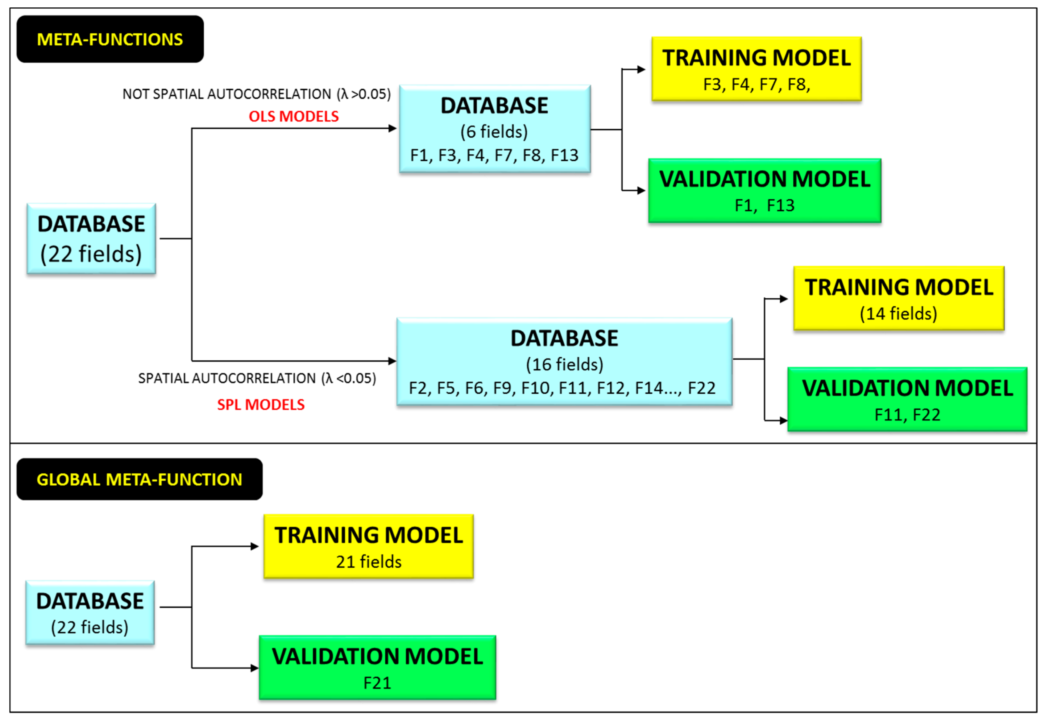
2.2. Data Analysis
3. Results
3.1. Spatial Autocorrelation on Yield and Imagery Data
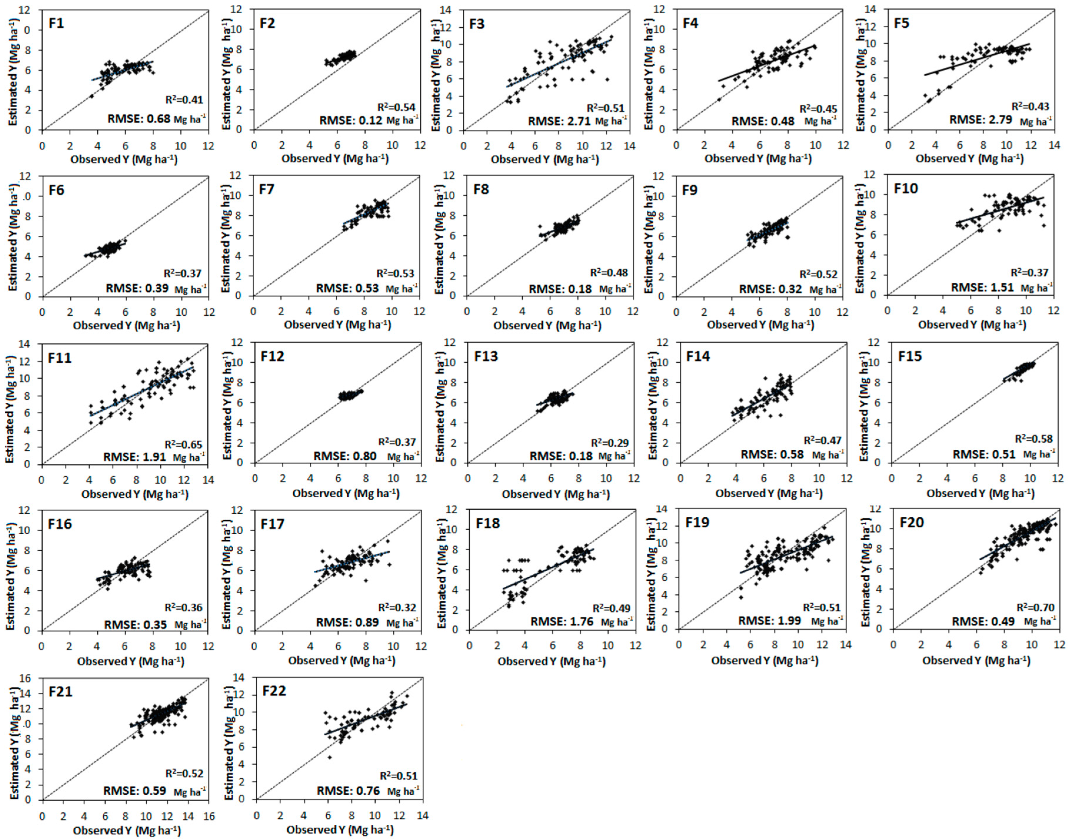
3.2. Comparison of Models for Relationship between Observed Yield and Satellite Data
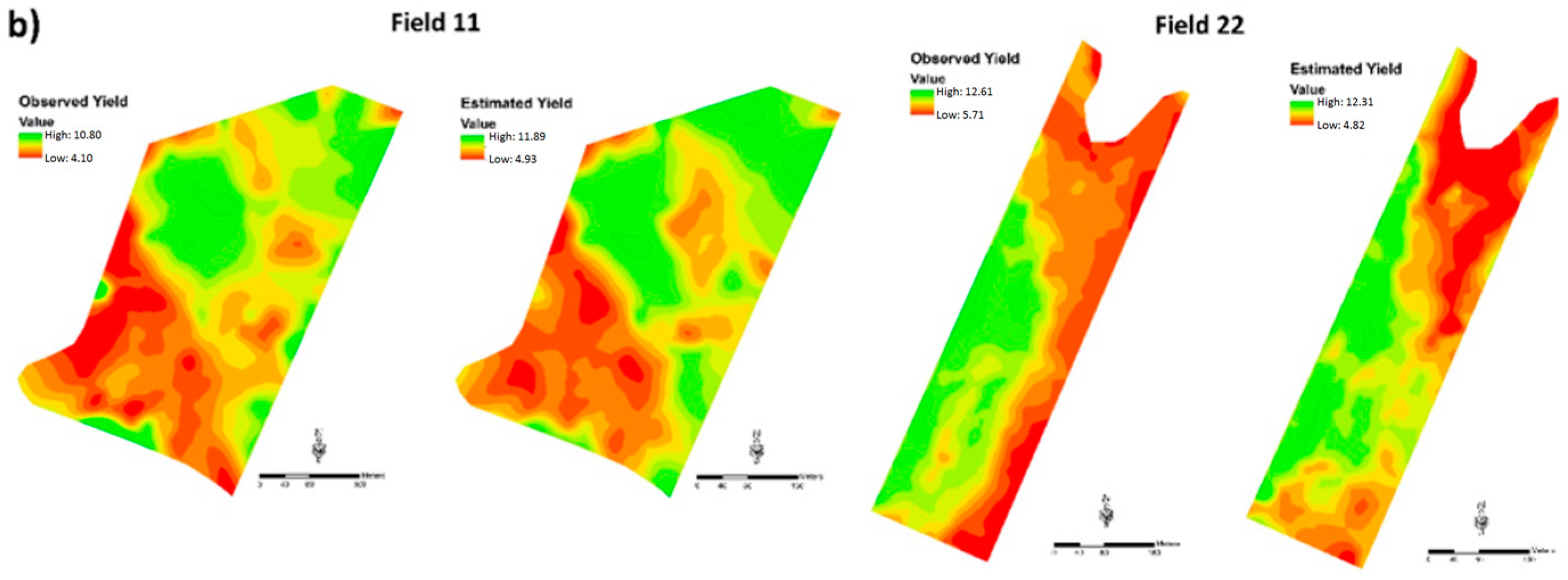
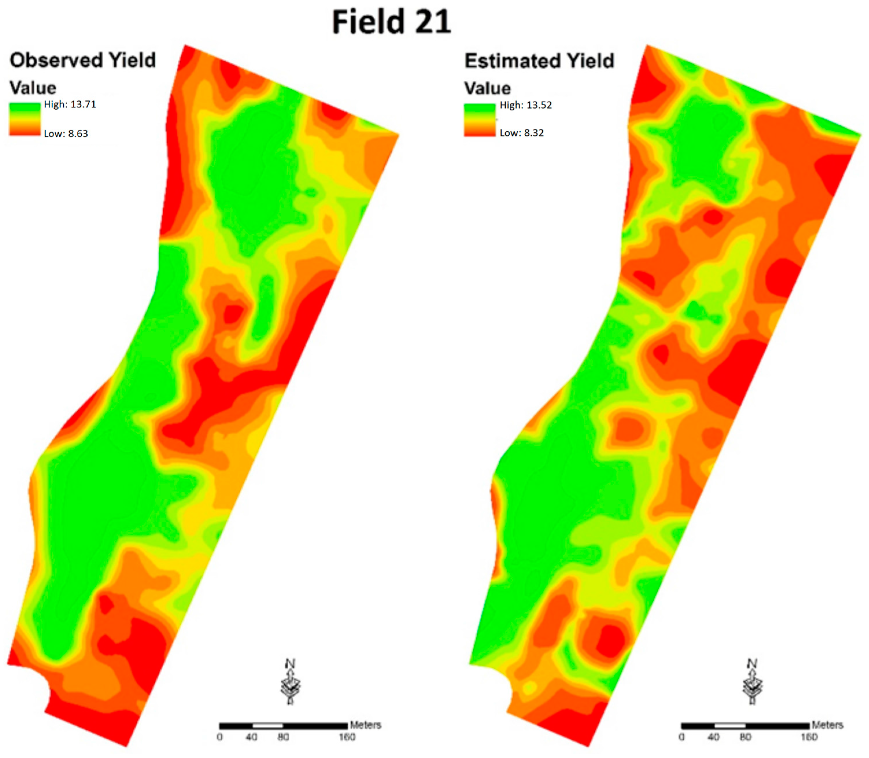
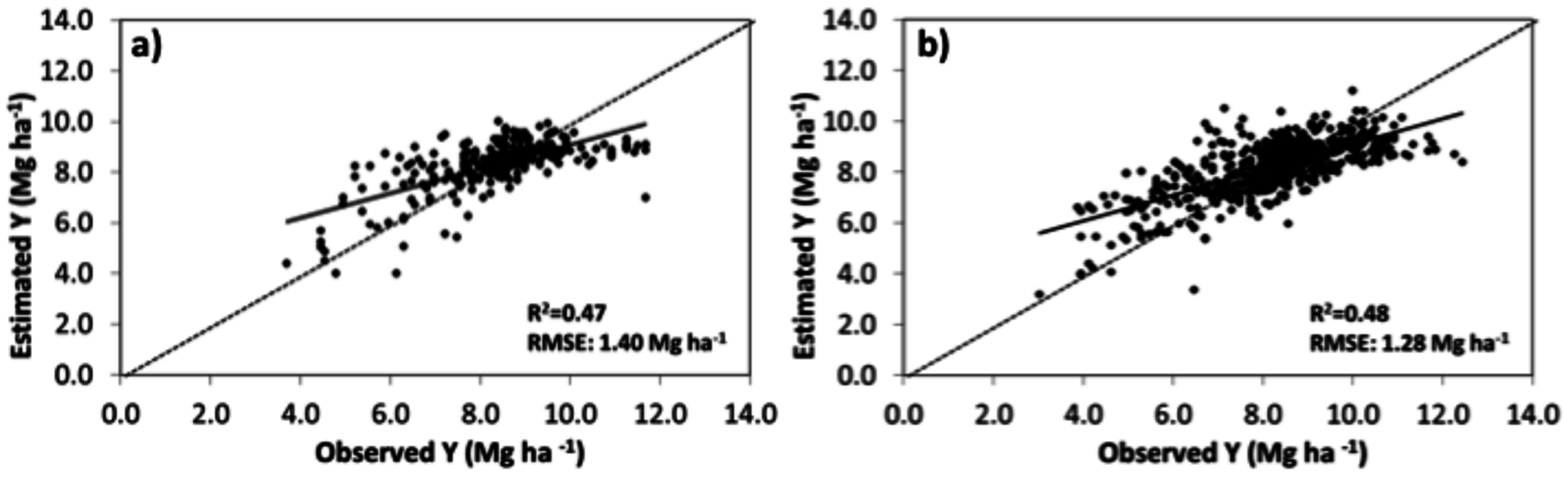
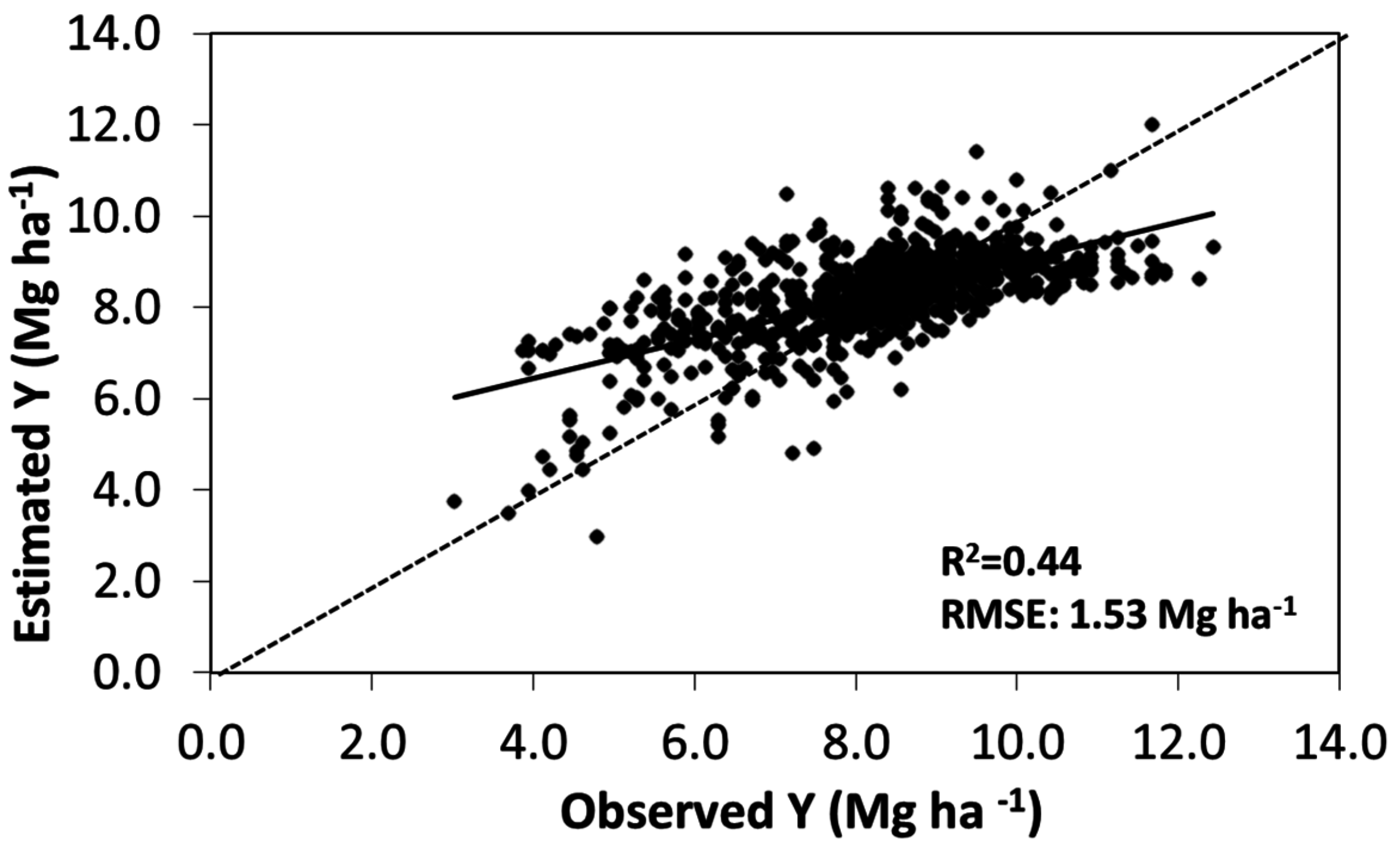
3.3. Spatial and OLS Model Variables and Validation Performance
with spatial coefficient 0.32 ***(λ)
4. Discussion
5. Conclusions
Acknowledgments
Author Contributions
Conflicts of Interest
References
- Hammer, G.L.; Hansen, J.W.; Phillips, J.G.; Mjelde, J.W.; Hill, H.; Love, A.; Potgieter, A. Advances in application of climate prediction in agriculture. Agric. Syst. 2001, 70, 515–553. [Google Scholar] [CrossRef]
- Kantanantha, N.; Serban, N.; Griffin, P. Yield and price forecasting for stochastic crop decision planning. J. Agric. Biol. Environ. Stat. 2010, 15, 362–380. [Google Scholar] [CrossRef]
- Stone, R.C.; Meinke, H. Operational seasonal forecasting of crop performance. Philos. Trans. R. Soc. Lond. B Biol. Sci. 2005, 360, 2109–2124. [Google Scholar] [CrossRef] [PubMed]
- Noureldin, N.A.; Aboelghar, M.A.; Saudy, H.S.; Ali, A.M. Rice yield forecasting models using satellite imagery in Egypt. Egypt. J. Remote Sens. Sp. Sci. 2013, 16, 125–131. [Google Scholar] [CrossRef]
- Assefa, Y.; Prasad, P.V.V.; Carter, P.; Hinds, M.; Bhalla, G. Yield responses to planting density for US modern corn hybrids: A synthesis-analysis. Crop Sci. 2016, 56, 2802–2817. [Google Scholar] [CrossRef]
- Pierce, F.J.; Nowak, P. Aspects of precision agriculture. Adv. Agron. 1999, 67, 1–85. [Google Scholar]
- Peralta, N.R.; Costa, J.L.; Balzarini, M.; Castro Franco, M.; Córdoba, M.; Bullock, D. Delineation of management zones to improve nitrogen management of wheat. Comput. Electron. Agric. 2015, 110, 103–113. [Google Scholar] [CrossRef]
- Peralta, N.R.; Costa, J.L. Delineation of management zones with soil apparent electrical conductivity to improve nutrient management. Comput. Electron. Agric. 2013, 99, 218–226. [Google Scholar] [CrossRef]
- Birrell, S.J.; Sudduth, K.A.; Borgelt, S.C. Comparison of sensors and techniques for crop yield mapping. Comput. Electron. Agric. 1996, 14, 215–233. [Google Scholar] [CrossRef]
- Kravchenko, A.N.; Bullock, D.G. Correlation of corn and soybean grain yield with topography and soil properties. Agron. J. 2000, 92, 75–83. [Google Scholar] [CrossRef]
- Sudduth, K.A.; Drummond, S.T. Yield editor. Agron. J. 2007, 99, 1471–1482. [Google Scholar] [CrossRef]
- Mulla, D.J. Twenty five years of remote sensing in precision agriculture: Key advances and remaining knowledge gaps. Biosyst. Eng. 2013, 114, 358–371. [Google Scholar] [CrossRef]
- Yang, C.; Everitt, J.H.; Du, Q.; Luo, B.; Chanussot, J. Using high-resolution airborne and satellite imagery to assess crop growth and yield variability for precision agriculture. Proc. IEEE 2013, 101, 582–592. [Google Scholar] [CrossRef]
- Haboudane, D.; Miller, J.R.; Pattey, E.; Zarco-Tejada, P.J.; Strachan, I.B. Hyperspectral vegetation indices and novel algorithms for predicting green LAI of crop canopies: Modeling and validation in the context of precision agriculture. Remote Sens. Environ. 2004, 90, 337–352. [Google Scholar] [CrossRef]
- Nguy-Robertson, A.; Gitelson, A.; Peng, Y.; Viña, A.; Arkebauer, T.; Rundquist, D. Green leaf area index estimation in maize and soybean: Combining vegetation indices to achieve maximal sensitivity. Agron. J. 2012, 104, 1336–1347. [Google Scholar] [CrossRef]
- Viña, A.; Gitelson, A.A.; Nguy-Robertson, A.L.; Peng, Y. Comparison of different vegetation indices for the remote assessment of green leaf area index of crops. Remote Sens. Environ. 2011, 115, 3468–3478. [Google Scholar] [CrossRef]
- Ramoelo, A.; Skidmore, A.K.; Cho, M.A.; Schlerf, M.; Mathieu, R.; Heitkönig, I.M. A. Regional estimation of savanna grass nitrogen using the red-edge band of the spaceborne RapidEye sensor. Int. J. Appl. Earth Obs. Geoinf. 2012, 19, 151–162. [Google Scholar] [CrossRef]
- Beckschäfer, P.; Fehrmann, L.; Harrison, R.D.; Xu, J.; Kleinn, C. Mapping leaf area index in subtropical upland ecosystems using RapidEye imagery and the randomForest algorithm. iForest-Biogeosci. For. 2014, 7. [Google Scholar] [CrossRef]
- Kross, A.; McNairn, H.; Lapen, D.; Sunohara, M.; Champagne, C. Assessment of RapidEye vegetation indices for estimation of leaf area index and biomass in corn and soybean crops. Int. J. Appl. Earth Obs. Geoinf. 2015, 34, 235–248. [Google Scholar] [CrossRef]
- Ali, M.; Montzka, C.; Stadler, A.; Menz, G.; Thonfeld, F.; Vereecken, H. Estimation and validation of RapidEye-based time-series of leaf area index for winter wheat in the Rur catchment (Germany). Remote Sens. 2015, 7, 2808–2831. [Google Scholar] [CrossRef]
- Lobell, D.B. The use of satellite data for crop yield gap analysis. Field Crops Res. 2013, 143, 56–64. [Google Scholar] [CrossRef]
- Zhao, Y.; Chen, X.; Cui, Z.; Lobell, D.B. Using satellite remote sensing to understand maize yield gaps in the North China Plain. Field Crops Res. 2015, 183, 31–42. [Google Scholar] [CrossRef]
- Rembold, F.; Atzberger, C.; Savin, I.; Rojas, O. Using low resolution satellite imagery for yield prediction and yield anomaly detection. Remote Sens. 2013, 5, 1704–1733. [Google Scholar] [CrossRef] [Green Version]
- Anselin, L.; Bongiovanni, R.; Lowenberg-DeBoer, J. A spatial econometric approach to the economics of site-specific nitrogen management in corn production. Am. J. Agric. Econ. 2004, 86, 675–687. [Google Scholar] [CrossRef]
- Lambert, D.M.; Lowenberg-Deboer, J.; Bongiovanni, R. A comparison of four spatial regression models for yield monitor data: A case study from Argentina. Precis. Agric. 2004, 5, 579–600. [Google Scholar] [CrossRef]
- Bongiovanni, R.G.; Robledo, C.W.; Lambert, D.M. Economics of site-specific nitrogen management for protein content in wheat. Comput. Electron. Agric. 2007, 58, 13–24. [Google Scholar] [CrossRef]
- Hamada, Y.; Ssegane, H.; Negri, M.C. Mapping intra-field yield variation using high resolution satellite imagery to integrate bioenergy and environmental stewardship in an agricultural watershed. Remote Sens. 2015, 7, 9753–9768. [Google Scholar] [CrossRef]
- USDA. Crop Production Historical Track Record; USDA, National Agriculture Statistics Services U.S. Goverment Print. Office: Washington, DC, USA, 2015.
- Ritchie, S.W.; Hanway, J.J. How a Corn Plant Develops; Iowa State University of Science and Technology, Cooperative Extension Service: Ames, IA, USA, 1989. [Google Scholar]
- Horowitz, J.; Ebel, R.; Ueda, K. No-Till Farming Is a Growing Practice; Economic Information Bulletin, Number 70; United States Department of Agriculture Economic Research Service: Washington, DC, USA, 2010.
- Rouse, J.W.; Haas, R.H.; Schell, J.A. Monitoring the Vernal Advancement and Retrogradation (Greenwave Effect) of Natural Vegetation; Texas A and M University: College Station, TX, USA, 1994. [Google Scholar]
- Gitelson, A.A.; Kaufman, Y.J.; Merzlyak, M.N. Use of a green channel in remote sensing of global vegetation from EOS-MODIS. Remote Sens. Environ. 1996, 58, 289–298. [Google Scholar] [CrossRef]
- Gitelson, A.; Merzlyak, M.N. Spectral reflectance changes associated with autumn senescence of Aesculus hippocastanum L. and Acer platanoides L. leaves. Spectral features and relation to chlorophyll estimation. J. Plant Physiol. 1994, 143, 286–292. [Google Scholar] [CrossRef]
- Peralta, N.R.; Costa, J.L.; Balzarini, M.; Franco, M.C.; Córdoba, M.; Bullock, D. Delineation of management zones to improve nitrogen management of wheat. Comput. Electron. Agric. 2015, 110, 103–113. [Google Scholar] [CrossRef]
- Peralta, N.R.; Costa, J.L.; Balzarini, M.; Angelini, H. Delineation of management zones with measurements of soil apparent electrical conductivity in the southeastern pampas. Can. J. Soil Sci. 2013, 93, 205–218. [Google Scholar] [CrossRef]
- Córdoba, M.A.; Bruno, C.I.; Costa, J.L.; Peralta, N.R.; Balzarini, M.G. Protocol for multivariate homogeneous zone delineation in precision agriculture. Biosyst. Eng. 2016, 143, 95–107. [Google Scholar] [CrossRef]
- Moran, P.A.P. Notes on continuous stochastic phenomena. Biometrika 1950, 37, 17–23. [Google Scholar] [CrossRef] [PubMed]
- Anselin, L. GeoDa, A Software Program for the Analysis of Spatial Data, Version 0.9. 5-i5 (Aug 3, 2004); Spatial Analysis Laboratory, Department of Agricultural and Consumer Economics, University of Illinois, Urbana-Champaign: Urbana, IL, USA, 2004. [Google Scholar]
- Cliff, A.; Ord, K. The Problem of Spatial Autocorrelation. In London Papers in Regional Science 1; Studies in Regional Science, 25–55; Scott, A.J., Ed.; Pion.: London, UK, 1969. [Google Scholar]
- Kitchen, N.R.; Sudduth, K.A.; Myers, D.B.; Drummond, S.T.; Hong, S.Y. Delineating productivity zones on claypan soil fields using apparent soil electrical conductivity. Comput. Electron. Agric. 2005, 46, 285–308. [Google Scholar] [CrossRef]
- Peralta, N.R.; Franco, C.; Costa, J.L.; Calandroni, M. Delimitation of management and relationship between soil apparent electrical conductivity and yield maps. In Proceedings of the 11th International Course on Precision Agriculture, Cordoba, Argentina, 18–20 July 2012.
- Willmott, C.J.; Ackleson, S.G.; Davis, R.E.; Feddema, J.J.; Klink, K.M.; Legates, D.R.; O’donnell, J.; Rowe, C.M. Statistics for the evaluation and comparison of models. J. Geophys. Res. 1985, 90, 8995–9005. [Google Scholar] [CrossRef]
- Searcy, S.W.; Schueller, J.K.; Bae, Y.H.; Borgelt, S.C.; Stout, B.A. Mapping of spatially variable yield during grain combining. Trans. ASAE 1989, 32, 826–829. [Google Scholar] [CrossRef]
- Yang, C.; Everitt, J.H.; Bradford, J.M. Comparisons of uniform and variable rate nitrogen and phosphorus fertilizer applications for grain sorghum. Trans. ASAE 2001, 44, 201–205. [Google Scholar] [CrossRef]
- Shanahan, J.; Schepers, J.S.; Francis, D.D.; Varvel, G.E.; Wilhelm, W.W.; Tringe, J.M.; Schlemmer, M.R.; Major, D.J. Use of remote-sensing imagery to estimate corn grain yield. Agron. J. 2001, 93, 583–589. [Google Scholar] [CrossRef]
- Timlin, D.J.; Pachepsky, Y.; Snyder, V.A.; Bryant, R.B. Spatial and temporal variability of corn grain yield on a hillslope. Soil Sci. Soc. Am. J. 1998, 62, 764–773. [Google Scholar] [CrossRef]
- Jaynes, D.B.; Colvin, T.S. Spatiotemporal variability of corn and soybean yield. Agron. J. 1997, 89, 30–37. [Google Scholar] [CrossRef]
- Bakhsh, A.; Jaynes, D.B.; Colvin, T.S.; Kanwar, R.S. Spatio-temporal analysis of yield variability for a corn-soybean field in Iowa. Trans. ASAE 2000, 43, 31–33. [Google Scholar] [CrossRef]
- Locke, C.R.; Carbone, G.J.; Filippi, A.M.; Sadler, E.J.; Gerwig, B.K.; Evans, D.E. Using remote sensing and modeling to measure crop biophysical variability. In Proceedings of the 5th International Conference on Precision Agriculture, City, Country, Bloomington, MN, USA, 16 July 2000.
- Hatfield, J.L.; Prueger, J.H. Value of using different vegetative indices to quantify agricultural crop characteristics at different growth stages under varying management practices. Remote Sens. 2010, 2, 562–578. [Google Scholar] [CrossRef]
- Sharma, L.K.; Bu, H.; Denton, A.; Franzen, D.W. Active-optical sensors using red NDVI compared to red edge NDVI for Prediction of corn grain yield in North Dakota, USA. Sensors 2015, 15, 27832–27853. [Google Scholar] [CrossRef] [PubMed]
- Sharma, L.K.; Franzen, D.W. Use of corn height to improve the relationship between active optical sensor readings and yield estimates. Precis. Agric. 2014, 15, 331–345. [Google Scholar] [CrossRef]
- Zhang, M.; Hendley, P.; Drost, D.; O’Neill, M.; Ustin, S. Corn and soybean yield indicators using remotely sensed vegetation index. Precis. Agric. 1999, 1999, 1475–1481. [Google Scholar]
- Dobermann, A.; Ping, J.L. Geostatistical integration of yield monitor data and remote sensing improves yield maps. Agron. J. 2004, 96, 285–297. [Google Scholar] [CrossRef]
- Huang, J.; Wang, X.; Li, X.; Tian, H.; Pan, Z. Remotely sensed rice yield prediction using multi-temporal NDVI data derived from NOAA’s-AVHRR. PLoS ONE 2013, 8, e70816. [Google Scholar] [CrossRef] [PubMed]
- Lopresti, M.F.; Di Bella, C.M.; Degioanni, A.J. Relationship between MODIS-NDVI data and wheat yield: A case study in Northern Buenos Aires province, Argentina. Inf. Process. Agric. 2015, 2, 73–84. [Google Scholar] [CrossRef]
- Cicek, H.; Sunohara, M.; Wilkes, G.; McNairn, H.; Pick, F.; Topp, E.; Lapen, D.R. Using vegetation indices from satellite remote sensing to assess corn and soybean response to controlled tile drainage. Agric. Water Manag. 2010, 98, 261–270. [Google Scholar] [CrossRef]
- Maddonni, G.A.; Otegui, M.E.; Cirilo, A.G. Plant population density, row spacing and hybrid effects on maize canopy architecture and light attenuation. Field Crop. Res. 2001, 71, 183–193. [Google Scholar] [CrossRef]
- Sadras, V.O.; Calviño, P.A. On-farm quantification of yield response to soil depth in soybean, maize, sunflower and wheat. Agron. J. 2001, 93, 577–583. [Google Scholar] [CrossRef]
- DiRienzo, C.; Fackler, P.; Goodwin, B.K. Modeling spatial dependence and spatial heterogeneity in county yield forecasting models. In Proceedings of the American Agricultural Economics Association Annual Meeting, Tampa, FL, USA, 1 August 2000.
- Ozaki, V.A.; Ghosh, S.K.; Goodwin, B.K.; Shirota, R. Spatio-temporal modeling of agricultural yield data with an application to pricing crop insurance contracts. Am. J. Agric. Econ. 2008, 90, 951–961. [Google Scholar] [CrossRef] [PubMed]
- Leiser, W.L.; Rattunde, H.F.; Piepho, H.; Parzies, H.K. Getting the most out of sorghum low-input field trials in west Africa using spatial adjustment. J. Agron. Crop Sci. 2012, 198, 349–359. [Google Scholar] [CrossRef]
- Richter, K.; Atzberger, C.; Vuolo, F.; D’Urso, G. Evaluation of sentinel-2 spectral sampling for radiative transfer model based LAI estimation of wheat, sugar beet, and maize. IEEE J. Sel. Top. Appl. Earth Obs. Remote Sens. 2011, 4, 458–464. [Google Scholar] [CrossRef]


| Field | County | Latitude(°) | Longitude (°) | Area (ha) | Imagery Acquisition (Date) | Final Yield (Mg·ha−1) | Yield Monitor (Year) |
|---|---|---|---|---|---|---|---|
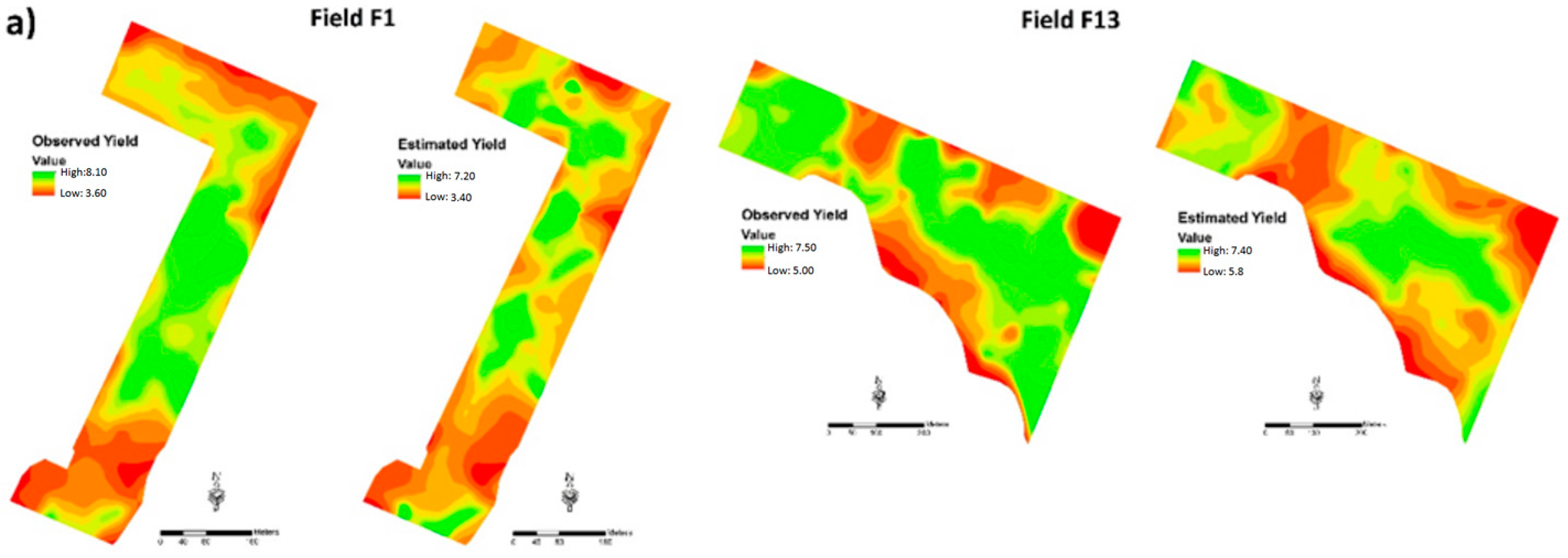
| F1 | Clay | −97.1561 | 39.5427 | 15 | 19 August 2013 | 6.0 | 2013 |
| F2 | Dickinson | −97.2091 | 39.0396 | 10 | 21 August 2015 | 6.6 | 2015 |
| F3 | Clay | −97.2430 | 39.5135 | 65 | 19 August 2013 | 8.6 | 2013 |
| F4 | Rice | −98.1857 | 38.3291 | 31 | 2 August 2014 | 7.1 | 2014 |
| F5 | Saline | −97.4505 | 38.6361 | 24 | 5 July 2015 | 8.6 | 2015 |
| F6 | Dickinson | −97.2369 | 39.0443 | 14 | 8 September 2011 | 4.8 | 2011 |
| F7 | Dickinson | −97.2934 | 39.0639 | 18 | 19 September 2013 | 8.8 | 2013 |
| F8 | Dickinson | −97.3178 | 38.9742 | 19 | 19 August 2013 | 6.9 | 2013 |
| F9 | Dickinson | −97.3179 | 38.9777 | 37 | 19 August 2013 | 6.8 | 2013 |
| F10 | Dickinson | −97.3222 | 38.9763 | 11 | 19 August 2012 | 8.6 | 2012 |
| F11 | Dickinson | −97.3510 | 38.9959 | 20 | 8 August 2012 | 8.9 | 2012 |
| F12 | Dickinson | −97.2547 | 39.0403 | 12 | 21 August 2015 | 6.7 | 2015 |
| F13 | Clay | −97.2331 | 39.5586 | 24 | 2 July 2011 | 6.4 | 2011 |
| F14 | Washington | −97.2068 | 39.5744 | 23 | 2 July 2012 | 6.3 | 2012 |
| F15 | Clay | −97.2173 | 39.5369 | 13 | 19 August 2013 | 9.5 | 2013 |
| F16 | Washington | −97.2132 | 39.5912 | 25 | 19 August 2013 | 6.1 | 2013 |
| F17 | Washington | −97.2151 | 39.5898 | 27 | 21 August 2013 | 7.0 | 2013 |
| F18 | Dickinson | −97.2467 | 39.0446 | 5 | 8 July 2014 | 6.2 | 2014 |
| F19 | Saline | −97.6010 | 38.6562 | 17 | 8 July 2014 | 8.7 | 2014 |
| F20 | Saline | −97.4254 | 38.7302 | 13 | 13 August 2013 | 9.5 | 2013 |
| F21 | Saline | −97.4379 | 38.7145 | 19 | 8 July 2013 | 11.5 | 2013 |
| F22 | Saline | −97.5983 | 38.6562 | 15 | 8 July 2014 | 9.1 | 2014 |
| Index | Abbreviation | Equation | Reference |
|---|---|---|---|
| Near infrared | NIR | ||
| Normalized difference vegetation index | NDVIr | (RNIR − RED)/(RNIR + RRED) | [31] |
| Green normalized difference vegetation index | NDVIG | (RNIR − RGREEN)/(RNIR + RGREEN) | [32] |
| Red-edge normalized difference vegetation index | NDVIre | (RNIR − REDEDGE)/(RNIR + RREDEDGE) | [33] |
| Red-edge simple radio | SRre | RNIR/REDEDGE | [33] |
| Field | NIR | SRre | NDVIr | NDVIG | NDVIre | Yield | ||||||
|---|---|---|---|---|---|---|---|---|---|---|---|---|
| MI | p-Value | MI | p-Value | MI | p-Value | MI | p-Value | MI | p-Value | MI | p-Value | |
| F1 | 0.13 | *** | 0.08 | * | 0.11 | *** | 0.12 | *** | 0.10 | ** | 0.08 | *** |
| F2 | 0.14 | *** | 0.10 | *** | 0.12 | *** | 0.10 | ** | 0.12 | *** | 0.09 | *** |
| F3 | 0.18 | *** | 0.15 | *** | 0.17 | *** | 0.16 | *** | 0.16 | *** | 0.12 | *** |
| F4 | 0.06 | * | 0.07 | ** | 0.05 | * | 0.06 | * | 0.09 | * | 0.09 | ** |
| F5 | 0.17 | *** | 0.14 | *** | 0.16 | *** | 0.18 | *** | 0.16 | *** | 0.13 | *** |
| F6 | 0.20 | *** | 0.20 | *** | 0.22 | *** | 0.20 | *** | 0.21 | *** | 0.25 | *** |
| F7 | 0.14 | *** | 0.10 | *** | 0.12 | *** | 0.10 | ** | 0.12 | *** | 0.09 | * |
| F8 | 0.10 | *** | 0.12 | *** | 0.13 | *** | 0.12 | *** | 0.13 | *** | 0.11 | ** |
| F9 | 0.13 | *** | 0.11 | *** | 0.11 | *** | 0.11 | *** | 0.12 | *** | 0.10 | ** |
| F10 | 0.19 | *** | 0.19 | *** | 0.20 | *** | 0.20 | *** | 0.19 | *** | 0.16 | *** |
| F11 | 0.28 | *** | 0.23 | *** | 0.29 | *** | 0.25 | *** | 0.26 | *** | 0.24 | *** |
| F12 | 0.24 | *** | 0.20 | *** | 0.21 | *** | 0.19 | *** | 0.17 | *** | 0.17 | *** |
| F13 | 0.16 | *** | 0.14 | *** | 0.12 | *** | 0.13 | *** | 0.12 | *** | 0.11 | *** |
| F14 | 0.06 | * | 0.07 | * | 0.08 | * | 0.07 | * | 0.08 | ** | 0.09 | ** |
| F15 | 0.14 | *** | 0.15 | *** | 0.14 | *** | 0.14 | *** | 0.15 | *** | 0.14 | *** |
| F16 | 0.13 | *** | 0.10 | ** | 0.11 | *** | 0.11 | *** | 0.12 | *** | 0.10 | *** |
| F17 | 0.15 | *** | 0.14 | *** | 0.14 | *** | 0.13 | *** | 0.12 | *** | 0.12 | *** |
| F18 | 0.16 | *** | 0.14 | *** | 0.16 | *** | 0.15 | *** | 0.15 | *** | 0.13 | *** |
| F19 | 0.12 | *** | 0.12 | *** | 0.13 | *** | 0.11 | *** | 0.12 | *** | 0.1 | ** |
| F20 | 0.16 | *** | 0.13 | *** | 0.14 | *** | 0.16 | *** | 0.14 | *** | 0.15 | *** |
| F21 | 0.14 | *** | 0.10 | ** | 0.12 | *** | 0.10 | *** | 0.12 | *** | 0.09 | *** |
| F22 | 0.29 | *** | 0.26 | *** | 0.25 | *** | 0.27 | *** | 0.27 | *** | 0.15 | *** |
| Field | Models | Equations | AIC | |
|---|---|---|---|---|
| F1 | OLS | Yield (Mg·ha−1) = −7.8 *** + 0.12(NIR)+20.0 ***(NDVIre) | 238.6 | |
| SPL | Yield (Mg·ha−1) = −6.9 *** + 0.11(NIR) + 20.2 ***(NDVIre)+ 0.28(λ) | 236.8 | ||
| F2 | OLS | Yield (Mg·ha−1) = −1.8 * + 8.2 **(NDVIG) + 1.16 ***(SRre) | 80.3 | |
| SPL | Yield (Mg·ha−1)= −0.3 + 7.8 **(NDVIG)+ 1.18 ***(SRre)+ 0.58 ***(λ) | 72.6 | ||
| F3 | OLS | Yield (Mg·ha−1)= −9.1 *** − 14.9 *(NDVI) + 26.5(NDVIG) + 34.0 ***(NDVIre) | 346.8 | |
| SPL | Yield (Mg·ha−1)= −9.2 *** − 14.7 *(NDVI) + 26.52(NDVIG) + 33.91 ***(NDVIre) − 0.06(λ) | 344.8 | ||
| F4 | OLS | Yield (Mg·ha−1) = −1.1 + 28.5 ***(NDVI) + 17.7(NDVIG) − 30.85 ***(NDVIre) | 284.2 | |
| SPL | Yield (Mg·ha−1) = −1.7 + 29.2 ***(NDVI) + 16.91(NDVIG) − 30.89 ***(NDVIre) + 0.23(Wu) | 281.9 | ||
| F5 | OLS | Yield (Mg·ha−1) = −4.8 *** + 23.6 ***(NDVI) | 391.4 | |
| SPL | Yield (Mg·ha−1) = −4.8 *** + 23.7 ***(NDVI) + 0.04 *(λ) | 391.3 | ||
| F6 | OLS | Yield (Mg·ha−1) = −0.9 * + 12.7 ***(NDVIG) | 108.2 | |
| SPL | Yield (Mg·ha−1) = −1.42 * + 13.8 ***(NDVIG) + 0.02 *(λ) | 104.2 | ||
| F7 | OLS | Yield (Mg·ha−1) = 3.5 ** + 0.12 **(NIR) | 106.8 | |
| SPL | Yield (Mg·ha−1) = 3.5 ** + 0.12 **(NIR) − 0.04(λ) | 106.6 | ||
| F8 | OLS | Yield (Mg·ha−1) = −3.1 *** + 2.2***(SRre) + 11.4***(NDVIG) | 110.5 | |
| SPL | Yield (Mg·ha−1) = −3.2 *** + 2.2 ***(SRre) + 11.7 ***(NDVIG) + 0.02(λ) | 110.5 | ||
| F9 | OLS | Yield (Mg·ha−1) = −4.69 *** + 0.95(NDVIG) + 24.1 ***(NDVIre) | 111.2 | |
| SPL | Yield (Mg·ha−1) = −4.7 *** + 0.47(NDVIG) + 24.5 ***(NDVIre) − 0.14 *(λ) | 110.5 | ||
| F10 | OLS | Yield (Mg·ha−1) = −8.6 ** + 0.57 ***(NIR) − 6.5 ***(SRre) + 20.8 ***(NDVIG) | 252.5 | |
| SPL | Yield (Mg·ha−1) = −8.1 ** + 0.48 ***(NIR) − 5.2 ***(SRre) + 21.5 ***(NDVIG) + 0.27 *(λ) | 250.0 | ||
| F11 | OLS | Yield (Mg·ha−1) = 0.46 + 32.36 ***(NDVIre) | 342.5 | |
| SPL | Yield (Mg·ha−1) = 0.53 + 32.09 ***(NDVIre) − 0.22 *(λ) | 341.8 | ||
| F12 | OLS | Yield (Mg·ha−1) = 2.2 * + 0.15 ***(NIR) − 7.4 ***(NDVIG) | 31.8 | |
| SPL | Yield (Mg·ha−1) = 2.0 * + 0.17 ***(NIR) − 9.6 **(NDVIG) + 0.39 *(λ) | 28.0 | ||
| F13 | OLS | Yield (Mg·ha−1)= −0.25 + 0.13 ***(NIR) + 22.9 ***(NDVIre) − 14.7 ***(NDVI) | 104.0 | |
| SPL | Yield (Mg·ha−1) = −0.15 + 0.12 ***(NIR) + 22.8 ***(NDVIre) − 14.6 ***(NDVI) + 0.09(λ) | 103.7 | ||
| F14 | OLS | Yield (Mg·ha−1) = −2.8 *** + 23.9 ***(NDVIre) | 239.0 | |
| SPL | Yield (Mg·ha−1) = −4.2 *** + 27.6 ***(NDVIre) + 0.63 ***(λ) | 220.6 | ||
| F15 | OLS | Yield (Mg·ha−1) = 4.1 *** + 5.1 ***(NDVI) + 4.9 ***(NDVIre) | 12.7 | |
| SPL | Yield (Mg·ha−1) = 3.1 *** + 6.0 ***(NDVI) + 5.9 ***(NDVIre) + 0.36 ***(λ) | 7.3 | ||
| F16 | OLS | Yield (Mg·ha−1) = −17.3 *** + 34.9 ***(SRre) + 16.7 ***(NDVIG) | 181.7 | |
| SPL | Yield (Mg·ha−1) = −18.7 *** + 33.7 ***(SRre) + 23.2 ***(NDVIG) + 0.71**(λ) | 165.5 | ||
| F17 | OLS | Yield (Mg·ha−1) = −12.4 *** + 31.4 ***(NDVI) | 236.3 | |
| SPL | Yield (Mg·ha−1) = −12.6 *** + 31.6 ***(NDVI) + 0.2 **(λ) | 234.5 | ||
| F18 | OLS | Yield (Mg·ha−1) = −26.5 *** + 17.8 ***(NDVI) + 41.8 ***(NDVIre) | 239.8 | |
| SPL | Yield (Mg·ha−1) = −26.4 *** + 20.8 ***(NDVI) + 37.8 ***(NDVIre) + 0.15 ***(λ) | 234.6 | ||
| F19 | OLS | Yield (Mg·ha−1) = −20.9 *** + 15.9(NDVI) + 36.1 ***(NDVIG) | 323.6 | |
| SPL | Yield (Mg·ha−1) = −20.0 *** + 17.2(NDVI) + 32.6 ***(NDVIG) + 0.39 **(λ) | 321.1 | ||
| F20 | OLS | Yield (Mg·ha−1) = −6.2 *** + 12.7 ***(NDVI) + 14.4 ***(NDVIre) | 348.2 | |
| SPL | Yield (Mg·ha−1) = −6.2 *** + 12.7 ***(NDVI) + 11.5 ***(NDVIre) + 0.21 *(λ) | 346.9 | ||
| F21 | OLS | Yield (Mg·ha−1) = −6.9 *** + 0.85 (SRre) + 6.0 **(NDVI) + 16.2 ***(NDVIG) + 12.1 ***(NDVIre) | 604.9 | |
| SPL | Yield (Mg·ha−1) = −7.1 *** + 0.69 (SRre) + 6.2 **(NDVI) + 14.6 ***(NDVIG) + 14.3 ***(NDVIre) + 0.35 ***(λ) | 592.5 | ||
| F22 | OLS | Yield (Mg·ha−1) = −21.59 *** + 57.38 ***(NDVIre) | 296.3 | |
| SPL | Yield (Mg·ha−1) = −20.07 *** + 54.47 ***(NDVIre)+ 0.27 ***(λ) | 292.5 | ||
| Models | Equations |
|---|---|
| OLS | Yield (Mg·ha−1)= −2.47 ** + 0.11 *(NIR) + 9.22 *(NDVIG) + 3.85 ***(NDVIre) |
| SPL | Yield (Mg·ha−1)= −10.43 ** + 0.31 **(NIR) − 9.21 *(NDVIG) + 16.59 ***(NDVIre) + 0.31 ***(λ) |
© 2016 by the authors; licensee MDPI, Basel, Switzerland. This article is an open access article distributed under the terms and conditions of the Creative Commons Attribution (CC-BY) license (http://creativecommons.org/licenses/by/4.0/).
Share and Cite
Peralta, N.R.; Assefa, Y.; Du, J.; Barden, C.J.; Ciampitti, I.A. Mid-Season High-Resolution Satellite Imagery for Forecasting Site-Specific Corn Yield. Remote Sens. 2016, 8, 848. https://doi.org/10.3390/rs8100848
Peralta NR, Assefa Y, Du J, Barden CJ, Ciampitti IA. Mid-Season High-Resolution Satellite Imagery for Forecasting Site-Specific Corn Yield. Remote Sensing. 2016; 8(10):848. https://doi.org/10.3390/rs8100848
Chicago/Turabian StylePeralta, Nahuel R., Yared Assefa, Juan Du, Charles J. Barden, and Ignacio A. Ciampitti. 2016. "Mid-Season High-Resolution Satellite Imagery for Forecasting Site-Specific Corn Yield" Remote Sensing 8, no. 10: 848. https://doi.org/10.3390/rs8100848