Post-Fire Changes in Forest Biomass Retrieved by Airborne LiDAR in Amazonia

Abstract

Fire is one of the main factors directly impacting Amazonian forest biomass and dynamics. Because of Amazonia’s large geographical extent, remote sensing techniques are required for comprehensively assessing forest fire impacts at the landscape level. In this context, Light Detection and Ranging (LiDAR) stands out as a technology capable of retrieving direct measurements of vegetation vertical arrangement, which can be directly associated with aboveground biomass. This work aims, for the first time, to quantify post-fire changes in forest canopy height and biomass using airborne LiDAR in western Amazonia. For this, the present study evaluated four areas located in the state of Acre, called Rio Branco, Humaitá, Bonal and Talismã. Rio Branco and Humaitá burned in 2005 and Bonal and Talismã burned in 2010. In these areas, we inventoried a total of 25 plots (0.25 ha each) in 2014. Humaitá and Talismã are located in an open forest with bamboo and Bonal and Rio Branco are located in a dense forest. Our results showed that even ten years after the fire event, there was no complete recovery of the height and biomass of the burned areas (p < 0.05). The percentage difference in height between control and burned sites was 2.23% for Rio Branco, 9.26% for Humaitá, 10.03% for Talismã and 20.25% for Bonal. All burned sites had significantly lower biomass values than control sites. In Rio Branco (ten years after fire), Humaitá (nine years after fire), Bonal (four years after fire) and Talismã (five years after fire) biomass was 6.71%, 13.66%, 17.89% and 22.69% lower than control sites, respectively. The total amount of biomass lost for the studied sites was 16,706.3 Mg, with an average loss of 4176.6 Mg for sites burned in 2005 and 2890 Mg for sites burned in 2010, with an average loss of 3615 Mg. Fire impact associated with tree mortality was clearly detected using LiDAR data up to ten years after the fire event. This study indicates that fire disturbance in the Amazon region can cause persistent above-ground biomass loss and subsequent reduction of forest carbon stocks. Continuous monitoring of burned forests is required for depicting the long-term recovery trajectory of fire-affected Amazonian forests.

1. Introduction

The Amazon is the world’s largest tropical forest, covering an area of about 5.4 million km² [1,2]. This biome has been hit by two major droughts at the beginning of the 21st century [3]. The first extreme drought occurred in 2005, which was associated with the anomalous warming of the tropical North Atlantic Ocean, related to the Atlantic Multidecadal Oscillation (AMO) [4]. The second drought, registered in 2010, was attributed to a combination of the El Niño Southern Oscillation (ENSO) with a positive phase of the AMO. These two events caused the intensification of the dry season in the Amazon region, with increased water deficits and reduction of air humidity [5,6,7]. The extended dry and hot weather conditions favored the occurrence of forest fires [8].

According to the data produced by the QUEIMADAS [9] project, which is developed by the National Institute for Space Research (INPE) , the number of active fire detections in the Brazilian Amazon for the years 2005 and 2010 increased by 67% and 16% in relation to the 2000–2014 mean. The increase of fire events recorded in these dry periods was related to land-use activities inducing the leakage of agricultural fires to neighboring forested areas [5].

Fire is one of the main factors causing degradation of Amazonian forests, due to its direct impact on forest structure and dynamics [10,11,12]. Fires are known to reduce forest biomass through direct combustion and mortality of trees [12], causing up to 40% loss of trees with diameter at breast height (DBH) greater than 10 cm. Moreover, fire-induced mortality of these individuals can be responsible for 23% to 31% decrease in forest canopy cover and 12% to 30% decrease in living forest biomass [13]. Fires can also alter forest diversity by causing a complete turnover of species [11,14].

The legacy of fire impacts is expected to be sustained for years following the fire event [14], as delayed mortality of large trees (DBH ≥ 50 cm) can promote up to 67% reduction in living biomass in relation to the remaining biomass one year after fire in central Amazonian forests [15]. Moreover, mortality rates in forests affected by fires are significantly different from zero, two to three years after the fire event [16]. Nevertheless, capturing these long-term impacts of fires on tropical forests in a systematic way remains a challenge because of the difficulty in obtaining complex forest structure information over large areas, as well as the frequency of fire events and ecological processes [15,17].

LiDAR technology, however, stands out among the variety of remote sensing technologies that could assist in resolving the issues highlighted previously. This technology can directly retrieve vegetation structure variables such as canopy height, number of individuals, and volume and crown diameter [18,19]. LiDAR can also be used for indirect biophysical measurements, such as estimates of forest biomass [20].

This study, hence, aims to quantify fire impacts on forest height and biomass in the southwestern Brazilian Amazon using LiDAR technology. Specifically, this work seeks to answer the following questions: (1) what is the magnitude of understory fire impacts on forest height and biomass up to 10 years after the event? (2) How do forest fires affect the frequency distribution of diameter and height of trees? (3) What is the total impact of fires on forest biomass in the study area?

Based on previous studies [15,21,22,23], we first hypothesize that (1) forest biomass and height should be lower in areas affected by fire four to five years prior the measurements (fire occurrence in 2010) in relation to unburned forests and that (2) forest biomass and height should be similar in areas affected by fire eight to ten years prior the measurements (fire occurrence in 2005) than in unburned forests, assuming that these areas already had time to recover their fire-affected forest structure.

2. Materials and Methods

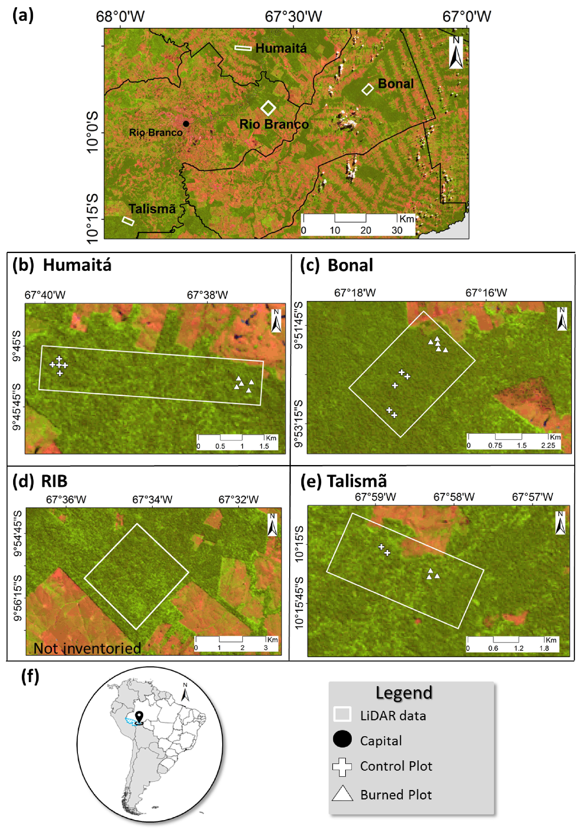
2.1. Study Area

Our survey focused on four sites affected by understory fires in southwestern Amazonia. The study sites were located in the eastern part of the state of Acre (Figure 1f). We selected two sites affected by understory fires in 2005, called Humaitá (Figure 1b) and Rio Branco (RIB) (Figure 1d). In addition to these two areas, we selected two sites affected by fires in 2010, called Bonal (Figure 1c) and Talismã (Figure 1e). Bonal and RIB are dominated by open submontane rainforest with bamboo and Humaitá and Talismã is characterized by dense submantane rainforest with emergent canopy [24,25]. The occurrence of fire events in this region was associated to two severe droughts that occurred in 2005 and 2010 [26,27,28,29]. During these events, fire incidence increased by 103.2% (2005) and 100.54% (2010) in relation to the long-term mean (2000–2014) [9] with an estimated area of degraded forest of 592 km² in 2005 and 259 km² in 2010 caused by the combination of logging and fire activities [30].

2.2. Burned Area Mapping

To locate burned sites within the LiDAR overpass region and perform subsequent analyses, we mapped burn scars for the years of 2005 and 2010 using images from TM (Thematic Mapper) sensor onboard Landsat-5 satellite and ETM+ (Enhanced Thematic Mapper Plus) sensor onboard Landsat-7 satellite, covering the period from June to November (when most active fire detections occurs, [12,31]) of these two years. To support identification of burn scars, we used surface reflectance images for the years of 2005 and 2010 from a Moderate Resolution Imaging Spectroradiometer (MODIS) sensor with 250 m resolution (Product MOD09). These images contain the best observation during an eight-day period [32].

The mapping of burned areas was carried out in two stages. In the first stage, fire scars were mapped based on visual interpretation of MODIS images (250 m spatial resolution). MODIS images were used due to their high temporal frequency, increasing the chances of acquiring cloud free images. Subsequently, to refine the boundaries of mapped burned areas, we used Landsat images with a 30 m spatial resolution. We first developed for all Landsat images linear spectral mixture models [33] to decompose each pixel into three components: soil, vegetation and shade. This procedure aimed to enhance the contrast between unburned and burned areas in the shade component, due to low reflectance of burned targets in all spectral bands [34,35]. In these images, the burned areas were also mapped based on visual interpretation. Finally, the total area burned for each studied region was mapped and quantified based on the integration of all burned polygons obtained from both MODIS and Landsat images. The total burned area mapped for RIB was of 442.14 ha (44.21%), Humaitá 119.78 ha (23.96%), Bonal was 149.69 ha (29.94%) and Talismã was 335.5 ha (55.92%).

2.3. Forest Inventory Data

Field plots were installed following a systematic design where the first field plot of each area was located randomly within the burned and unburned polygons identified from satellite data in each one of the surveyed areas. Taking the first field plot as a reference, the subsequent plots were set up following a cross design, with four plots located at the vertices of a square-like area and one plot in the middle (total of five plots per site). Each field plot was set up with a distance at least 70 m away from the central plot. The Talismã area was an exception. Due to logistical issues, we only set up two plots in the unburned area and three plots in the burned area, despite following the same experimental design. Forest inventory data were collected in 25 plots with an area of 0.25 ha (50 m × 50 m) each during June and July 2014. At Humaitá (Figure 1b) and Bonal (Figure 1c) study sites, we surveyed a total of 20 plots, with five plots per site set up in unburned forests (Control Areas—CA) paired with another cluster of five plots per site in forests affected by understory fire (Burned Areas—BA). At the Talismã study site, we surveyed a total of five plots (two plots in unburned areas and three plots in burned areas) (Figure 1e. Within each plot, we installed a subplot of 0.05 ha (10 m × 50 m). In these subplots, we measured DBH (stem diameter measured at 1.30 m above the ground level) and the total height of all trees with DBH larger than or equal to 10 cm. In the remaining 0.20 ha (40 m × 50 m) of the plot, we only measured the DBH and the total height of trees with DBH greater than or equal to 35 cm. All trees sampled were identified at least at the family level. The 2014 field campaign at the Humaitá study site allowed data collection representing nine years after the fire event, while data collection at Bonal and Talismã corresponded to four years of post-fire impact. All plots were geo-located using a differential Global Navigation Satellite System (GNSS). Geographical coordinates were measured at each one of the plot’s vertices with an average positioning error of 59 cm. In addition to the sites described above, we also used in our analysis LiDAR data for the RIB site (Figure 1d) to evaluate landscape level fire impact on height and biomass. However, no field data were collected at this site.

2.4. Field-Based Biomass Estimation

To calculate the biomass of each tree in each one of the 25 field plots, the equation developed by Chave et al. [36] was used (Equation (1)):

$$AG{B}_{est}=0.0673\times {\left(\rho D^{2}H\right)}^{0.976},$$

(1)

where $AG{B}_{est}$ corresponds to the aboveground biomass in kg; D is the DBH in cm, H is the total height in meters and ρ is the wood density in g/cm³. A wood density value for each tree identified in the field was established according to its species, genera or family name, based on the wood density database provided by [37].

To extrapolate the AGB of each tree for the whole plot, we used Equation (2). This calculation was adopted because only individuals with DBH greater than or equal to 35 cm were measured in the whole extent of the 50 m × 50 m plots. The calculation assumed that the partial sum of AGB for individuals with DBH < 35 cm measured at the 10 m × 50 m subplot was equally distributed across the whole 50 m × 50 m plot. Following this assumption, we multiplied the partial sum of AGB for individuals with DBH < 35 cm by five, and then we added this value to the partial sum of AGB for individuals with DBH ≥ 35 cm:

$$AG{B}_{plot}=5\times {\displaystyle \sum _i}AG{B}_i^{<35}+{\displaystyle \sum _i}AG{B}_i^{\ge 35},$$

(2)

where $AG{B}_{plot}$ corresponds to the total aboveground biomass of the field plot in kg, ${\sum }_{i}AG{B}_i^{<35}$ is the partial sum of biomass of the trees with DBH < 35 cm, and ${\sum }_{i}AG{B}_i^{\ge 35}$ is the partial sum of biomass of the trees with DBH ≥ 35 cm. This same approach was used to extrapolate the average height and the average DBH of each tree for the full extent of each field plot.

To calculate wood density for each plot, we used a weighted average. This value was calculated using the replication of trees with DBH < 35 cm in all plots and considering the basal area of the trees.

2.5. LiDAR Dataset

Airborne LiDAR data for this study were acquired with an Optec Orion instrument using a laser pulse emitted in the near infrared wavelength (1064 nm). This wavelength is used because vegetation targets have their highest reflectance in this region of the electromagnetic spectra, providing, therefore, a better returning signal to the LiDAR in relation to other wavelengths. In this wavelength, signal loss through scattering and absorption by the atmosphere is reduced; however, absorption of the signal by clouds is unavoidable, preventing the use of this wavelength in overcast conditions [38].

LiDAR acquisition campaigns were carried out in 2013 for Humaitá and Bonal, in 2014 for Talismã, and 2015 for RIB sites. These datasets are part of the Sustainable Landscapes Project. The total ground area covered by LiDAR data was 2600 ha for the four sites: Humaitá (500 ha), Talismã (500 ha), Bonal (600 ha) and RIB (1000 ha). The average density of laser returns was 66.61 points per square meter (ppm²) for Humaitá, 33.41 ppm² for Bonal, 40.7 ppm² for Talismã and 71.74 ppm² for RIB. The ideal point density for forest structure and biomass estimation studies was estimated to be at least four returns per square meter [39]. Here, we estimated that 96.26% , 92.02% , 96.15% and 99.98% of the area covered by the LiDAR in Humaitá, Bonal, Talismã and RIB, respectively, was in conformity with this specification.

Table 1. Laser system parameters for LiDAR data collection.

Parameter	Specification
Instrument	Optec Orion
Position system	APPLANIX 09SEN243
Average flight altitude	900 m
System frequency	100 kHz
Scan frequency	61.4 Hz
Scan Angle	11.1°
Overlap between flight lines	65%
Beam divergence	0.25 mrad

presents a detailed description of flight parameters for LiDAR data collection.

2.5.1. LiDAR Data Processing

LiDAR is an active remote sensing technology that can be operated either from ground, airborne or space-borne platforms [40,41,42,43]. In general, the LIDAR system emits a laser beam toward a surface and records the time required for the emitted pulse to travel from the laser source to the target and return to the sensor [44]. The product provided by the LIDAR is a point cloud with the geographic position (x and y) and height value (z) of each point on the Earth’s imaged surface [45,46].

Consistent data acquisition with low variability of flight height and high pulse density are fundamental to make LIDAR-derived metrics more robust and comparable across data sets [47]. The LiDAR metrics most frequently used in the estimation of forest biomass are mean or maximum canopy height, vertical canopy profile metrics, such as height percentiles and top-of-canopy height [48,49,50,51,52] . Typical methods to predict AGB with LiDAR data are based on regression models quantifying the relationship between LiDAR metrics and field-based plot-level estimates of biomass [19,20,53,54,55]. In additon, LiDAR data are sensitive to important differences in canopy structure over a wide range of conditions (i.e., from young secondary forests to primary tropical rainforests) [20].

In this work, LiDAR data were processed using the FUSION software (version 3.50) [56]. This tool was used to extract the following information from LiDAR data: number of returns, canopy height, intensity and topographical data. The height of the trees was calculated as the difference between the Canopy Surface Model (DCM) and the Digital Terrain Model (DTM) [50,57]. The products extracted from LiDAR to calculate forest biomass were: canopy height, average of height, third quartile of height, tenth percentile of height and kurtosis of the distribution of all return heights. LiDAR metrics were computed on regular 50 m × 50 m grids following the methodology of [58].

Forest biomass maps were produced by applying Equation (3) proposed by Longo et al. [58]. This equation was specifically developed for forests and degraded forests of the Brazilian Amazon. The model for estimation of forest biomass from LiDAR metrics explained 69% of the total variance across forest types, with a root mean square error of 4.27 kg·m⁻². More details can be found in Longo et al. [58]:

$$AG{B}_{LiDAR}=0.36{\mu }_z^{1.16}{z}_{75}^{0.78}{z}_{10}^{-0.18}{k}_z^{0.41},$$

(3)

where $AG{B}_{LiDAR}$ corresponds to the aboveground model based on airborne- LiDAR in Kg, ${\mu }_z$ is the mean of height, $z_{75}$ is the third quartile of height, $z_{10}$ is the tenth percentile of height, and $k_z$ is the kurtosis of the distribution of all return heights.

2.6. Statistical Analyses

For the data analyses, we grouped all the unburned areas of Humaitá, Bonal and Talismã to form our control area samples (CA). We also created two other groups of samples: (1) BA-2005: for the group of burned areas of Humaitá, and RIB; and (2) BA-2010: for the group of burned areas of Bonal and Talismã. The Kruskal–Wallis test was used to compare the distribution of DBH, height and biomass among the study sites.

The best regression model developed by Longo et al. [58] was selected based on the Bayesian Information Criterion (BIC). To evaluate the model robustness and quantify errors associated with independent predictions of aboveground biomass, a cross-validation test was applied based on 1000 bootstrap samplings [58].

We also applied a linear regression between biomass values estimated from the LiDAR data and years since the last fire occurrence to quantify changes in forest biomass as a function of the time after the fire event. From the fitted equation, we used the regression slope to depict the annual rate of biomass change following the fire event. Moreover, the intercept of the regression allowed for assessing the impact of fire on the biomass immediately after the occurrence of the event (time value approaching zero).

3. Results

3.1. Analysis of Field Plot

The average tree density was 321 trees per hectare (trees/ha) for CA, 291 trees/ha for BA-2005 and 298 trees/ha for BA-2010. These results showed that, despite the lower tree density (around 10%) in plots affected by fire four and nine years prior to the measurements, the areas are statistically similar in terms of density of trees.

Analyzing the percentage of trees per hectare by diameter class, we observed an inverted-J pattern in CA. This pattern is expected for uneven-aged stands and natural forests where a large number of trees populate the smaller diameter classes, following an exponential decrease in the number of trees with larger diameters [59] (Figure 2). Burned sites, BA-2005 (75%) and BA-2010 (77%), however, had a larger percent of trees than CA (71%) populating the smaller diameter class (10 ≤ DBH ≤ 25 cm). Conversely, both BA-2005 (15%) and BA-2010 (16%) had a lower number of trees in the 25 < DBH ≤ 40 cm size class in comparison to CA (21%). The percentage of trees with DBH > 40 cm for CA, BA-2005 and BA-2010 were 8%, 9% and 7%, respectively.

Field-based aboveground biomass (AGB), calculated using Equation (1), was 78.8 Mg·ha⁻¹ for CA, 152.9 Mg·ha⁻¹ for BA-2005 and 141.9 Mg·ha⁻¹ for BA-2010 (Figure 3). We observed a biomass loss of 25.9 Mg·ha⁻¹ for BA-2005 and 36.9 Mg·ha⁻¹ for BA-2010 when compared with CA. These values represented a percentage decrease of 14.49% for BA-2005 and 20.64% for BA-2010 when compared with CA. Comparing BA-2005 with BA-2010, the biomass loss was 11 Mg·ha⁻¹, which represents a reduction of 7.19%. There was no significant difference between the distribution of AGB of CA and BA-2005 (p-value = 0.16). On the other hand, there was a significant difference (p-value < 0.05) between CA and BA-2010 and between BA-2005 and BA-2010.

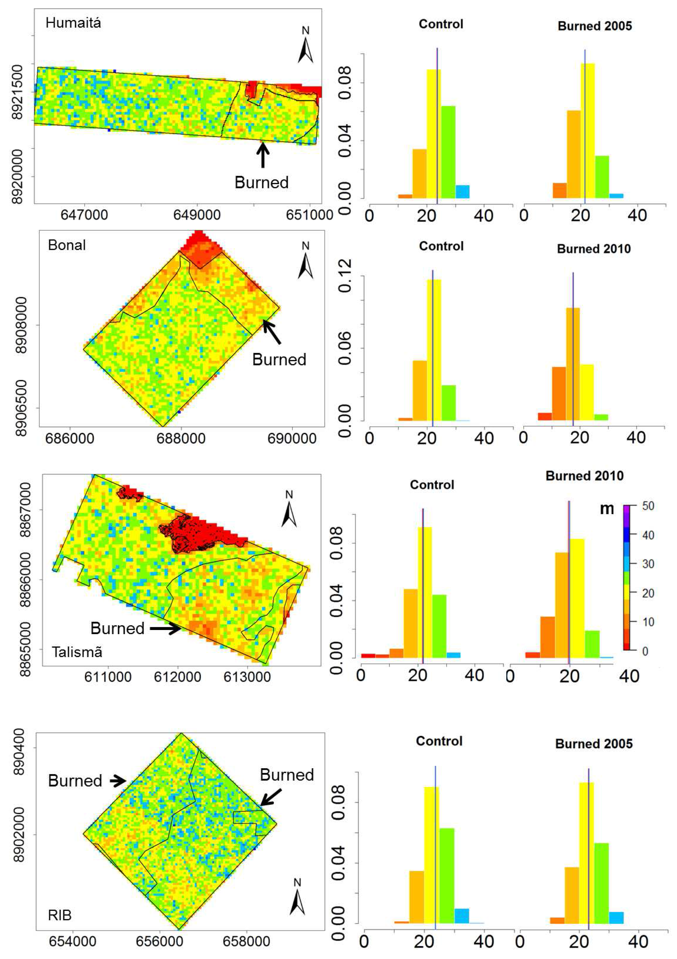
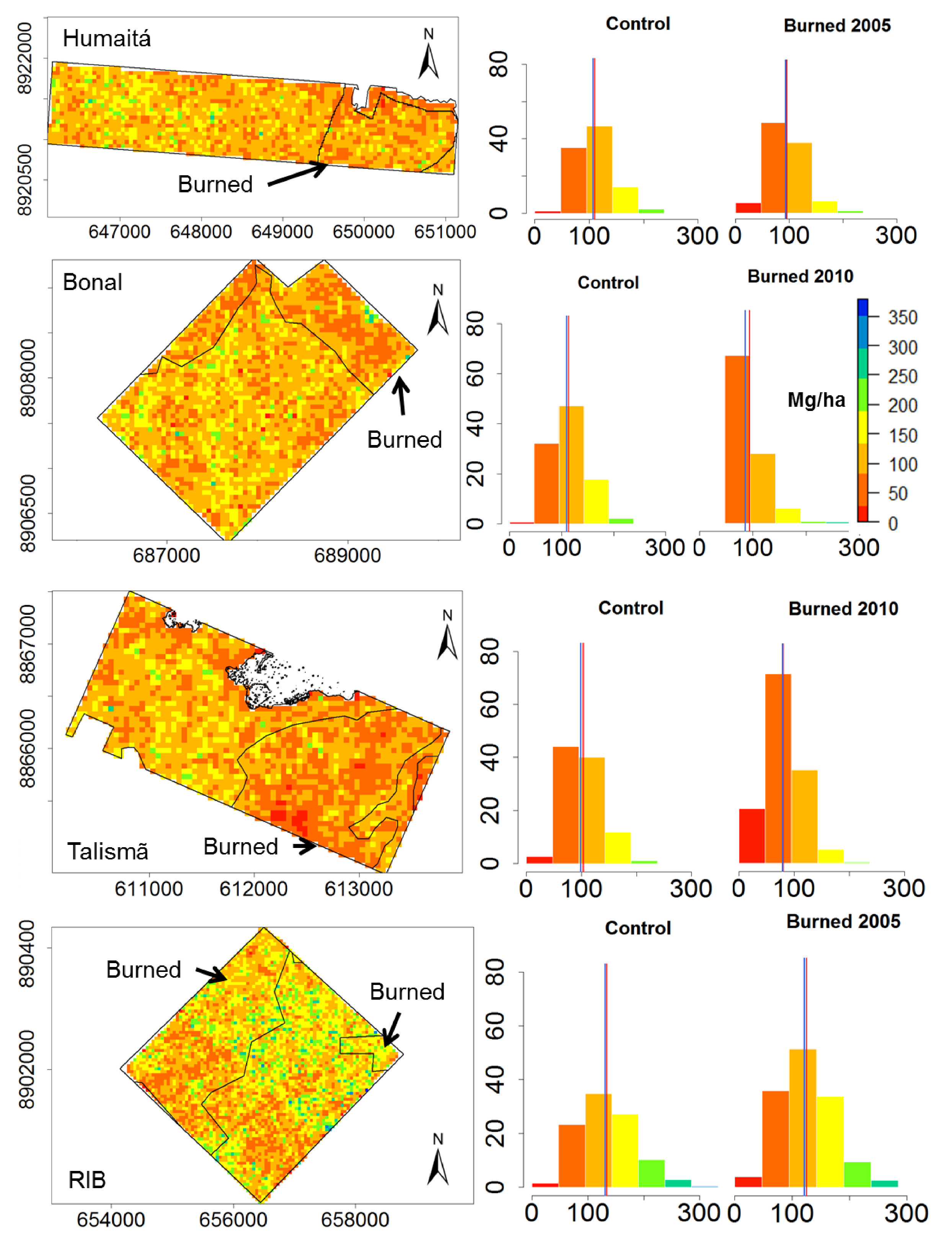
3.2. Analysis of LiDAR Data

Analyzing the LiDAR-derived height values, we found significant differences between the height distribution of CA and BA-2005, CA and BA-2010, and BA-2005 and BA-2010 (p-value < 0.05). For burned areas in 2005, the average height was 23.54 m (control) and 23.66 m (burned) for Humaitá and 21.36 m (control) and 23.11 m (burned) for RIB . For burned areas in 2010, the average height was 21.93 m (control) and 21.73 m (burned) for Bonal and 17.49 m (control) and 19.55 m (burned) for Talismã. Figure 4 shows the maps of height from LiDAR resampled to a regular 50 m × 50 m grid.

Differently from field-based measurements, we found significant differences between the distribution of AGB of CA and BA-2005, CA and BA-2010, and BA-2005 and BA-2010 (p-value < 0.05) , when analyzing the whole landscape affected by fire using LiDAR information. For burned areas in 2005, we observed a biomass loss of 8.99 Mg·ha⁻¹ for RIB (6.71% decrease) and 15.07 Mg·ha⁻¹ for Humaitá (13.66% decrease). For burned areas in 2010, we found a biomass loss of 20.39 Mg·ha⁻¹ for Bonal (17.89% decrease) and 23.47 Mg·ha⁻¹ for Talismã (22.69% decrease). The total forest biomass loss was 12,505.02 Mg for the four studies areas, with an average loss of 2890 Mg for sites burned in 2005 and 5463.2 Mg for sites burned in 2010, and with an average loss of 4176.6 Mg. Figure 5 shows the maps of AGB from LiDAR resampled to a regular 50 m × 50 m grid.

Table 2. Summary statistics from estimated aboveground biomass and Height by LiDAR data for Humaitá, Bonal, Talismã and Rio Branco. Mean and Median in Mg·ha⁻¹.

Sites	Years of Occurrence of Fire	Height (m)		AGB (Mg·ha−1)
		Control Mean ± stdev	Burned Mean ± stdev	Control Mean ± stdev	Burned Mean ± stdev
		RIB	2005	23.66 ± 3.90	23.13 ± 3.99	134.03 ± 50.61	125.04 ± 46.89
Humaitá	2005	23.54 ± 3.96	21.36 ± 3.82	110.35 ± 35.44	95.28 ± 32.60
Bonal	2010	21.93 ± 3.02	17.49 ± 3.99	113.95 ± 34.37	93.56 ± 30.97
Talismã	2010	21.73 ± 4.81	19.55 ± 4.50	103.46 ± 34.20	79.99 ± 32.72

presents the statistics from estimated height and AGB by LiDAR data for each area.

Exploring the relationship showing changes in the original biomass as a function of years since the last fire. It is interesting to note that if the recovery process followed a linear pattern ($R^2$ = 0.95, p < 0.01), burned forests would recover its original biomass at a rate of 1.84% a year (Figure 6) based on the slope of the regression. Moreover, the loss of biomass of the studied forests immediately after fire occurrence is likely to correspond to 27% of the original biomass according to the intercept of the regression.

4. Discussion

In this study, we showed for the first time that LIDAR technology is able to detect changes in forest biomass and height for a period equivalent to at least 10 years after the occurrence of an understory fire event. Fire impact on these forests, directly associated to the mortality of trees, is clearly differentiated using LIDAR data during the years succeeding the fire event. The difference between the results obtained from field and LiDAR data can be related to the low sample size of field data. Differently from field-based quantification of forest fire impacts, airborne LiDAR is capable of surveying larger areas allowing the detection of changes in forest structure, such as canopy gaps, which directly influence forest biomass after the occurrence of disturbances caused by fire. These findings confirm that fire-related impacts in Amazonian forests are more persistent than previously recorded in the literature (up to three years; [15]). However, very little is still known about the fate of forest biomass and carbon stocks following forest fire events considering the long-term dynamics of vegetation that remain in these areas [15,16]. LiDAR, therefore, is a powerful technology to further explore these impacts.

Forest biomass values estimated from LiDAR data in this study were consistent with our field biomass values. The mean biomass of the four forest sites analyzed in this study (114.45 ± 43.66 Mg·ha⁻¹) was lower than the mean biomass of Amazonian forests (318.4 Mg·ha⁻¹ [60]; 305.3 Mg·ha⁻¹ [61]; and 290.5 Mg·ha⁻¹ [62]). Our values, however, are in agreement with results from other forests with bamboo presence [63]. Several authors associate the reduced biomass of western Amazonian forests to the presence of bamboo [64,65,66]. Bamboo tends to reduce density and basal area of trees [67,68], restraining forest biomass development due to a negative feedback with the recruitment, growth, and survival of other individuals [69,70]. Tree recruitment is suppressed by the low density of seedlings and saplings [71,72,73,74].

Similar to other studies [22,23,75], we showed a significant biomass reduction in forest affected by fire. More interestingly, our LIDAR analysis allowed the detection of subtle changes in the canopy of burned sites in subsequent years after fire. LIDAR analysis showed that unburned sites had a significantly higher biomass than the sites that burned in 2005 and 2010. Moreover, sites that burned in 2005 had significantly higher biomass than sites burned in 2010. These results clearly demonstrate the persistent loss of biomass up to 10 years after fire. We estimated that initial loss of biomass from understory forest fire is equivalent to 27% of the original biomass value, with a succeeding recovery of forest biomass with a rate of 1.84% year⁻¹. It is interesting to note that field-based measurements of biomass are unable to detect the landscape scale changes in post-fire biomass. Despite finding a significant lower mean biomass for sites burned in 2010 in relation to the biomass of 2005 burned sites and control sites, we did not observe significant differences between biomass measured in 2005 burned and control sites.

Field-based measurements indicate that the reduction in the biomass of burned forests recorded by our field and LiDAR analyses is associated with a rearrangement of the diameter distribution of trees in the different diameter classes. The percentage of trees with small diameter (10 ≤ DBH ≤ 25 cm) tended to increase in areas affected by fires five and nine years prior to field measurements. This clearly demonstrated the regeneration process within burned sites [15]. The opposite behavior is observed in trees with diameters between 25 < DBH ≤ 40 cm . In this diameter class, the percentage of trees tended to decrease in areas affected by fire. This reduction is related to the delayed recovery time of trees to populate this diameter class. In most of the cases found in this diameter class, sites that burned in 2005 had a higher percentage of trees than sites burned in 2010. In most of the cases of this diameter class, sites that burned in 2005 had a higher percentage of trees than sites burned in 2010. We observed an exception for the 25–30 cm diameter class, as sites that burned in 2005 had fewer trees than sites that burned in 2010. The percentage reduction of trees can be related to late mortality [15,22,68]. A better understanding of this delayed mortality pattern is likely to be achievable through the continuous monitoring of the 2010 burned sites.

Surprisingly, we did not detect the impact of fire on large trees (DBH > 40 cm). Apparently, the intensity of fires in the studied area was not enough to impact the survivorship of large trees and the distribution pattern of these individuals yet. As expected, our field-based measurements show that these trees store the highest proportion of the aboveground biomass [22,36,76].

5. Conclusions

These results confirmed our first hypothesis that four to six years after fire, forest biomass and height were not yet recovered. Surprisingly, we demonstrate with the LiDAR analysis that even eight to 10 years after fire, forest biomass and height are not fully recovered. This finding rejects our second hypothesis and opens a new perspective on the long-term persistence of understory fire effects on tropical forests. We firmly recognize that Amazonian burned forests are likely to play an important role in the Amazonian forest carbon budget for at least 10 years after fire, due to the biomass loss and recovery dynamics of these forests observed here.

These results highlight the need for a larger sample size when carrying out field measurements for detecting these temporally dynamic subtle changes in post-fire forest biomass. LiDAR data, however, allows the retrieval of structural forest biophysical parameters over a much larger geographical extent than plot-based work does. LiDAR data, for instance, account for fire-induced gap formation, which is normally not contemplated by plot-based measurements. We advocate that LiDAR data is essential complementary information for landscape level estimates of post-fire biomass loss and recovery of tropical forests.

Continuous monitoring of burned forests at regional scales in Amazonia is critical for quantifying long-term impacts of fires not only on biomass and forest structure, but also for depicting changes in biodiversity [13]. LiDAR technology applied for tropical forest studies allow the mapping of forest biomass in areas with high tree density and with difficult access for conducting forest inventories. The results presented in this work can serve as a basis for future evaluations of fire impact between different types of forest in the Brazilian Amazon. Finally, the results found in this work can contribute to the perspective of the REDD (Reducing Emissions from Deforestation and Forest Degradation) mechanism and contribute to understanding and quantifying the dynamics of carbon stocks in burned areas [77,78,79].

References

1. Clement, C.R.; Higuchi, N. A floresta amazônica e o futuro do Brasil. Ciência Cultura 2006, 58, 44–49. [Google Scholar]
2. Nobre, C.A.; Sampaio, G.; Salazar, L. Mudanças climáticas e Amazônia. Ciência Cultura 2007, 59, 22–27. [Google Scholar]
3. Bi, J.; Myneni, R.; Lyapustin, A.; Wang, Y.; Park, T.; Chi, C.; Yan, K.; Knyazikhin, Y. Amazon forests’ response to droughts: A perspective from the MAIAC product. Remote Sens. 2016, 8. [Google Scholar] [CrossRef]
4. Marengo, J.A.; Nobre, C.A.; Tomasella, J.; Oyama, M.D.; Oliveira, G.S.; de Oliveira, R.; Camargo, H.; Alves, L.M.; Brown, I.F. The drought of Amazonia in 2005. J. Clim. 2008, 21, 495–516. [Google Scholar] [CrossRef]
5. Aragão, L.E.O.C.; Poulter, B.; Barlow, J.B.; Anderson, L.O.; Malhi, Y.; Saatchi, S.; Phillips, O.L.; Gloor, E. Environmental change and the carbon balance of Amazonian forests. Biol. Rev. 2014, 89, 913–931. [Google Scholar] [CrossRef] [PubMed]
6. Marengo, J.A.; Tomasella, J.; Alves, L.M.; Soares, W.R.; Rodriguez, D.A. The drought of 2010 in the context of historical droughts in the Amazon region. Geophys. Res. Lett. 2011, 38. [Google Scholar] [CrossRef]
7. Lewis, S.L.; Brando, P.M.; Phillips, O.L.; van der Heijden, G.M.F.; Nepstad, D. The 2010 Amazon drought. Science 2011, 331, 554. [Google Scholar] [CrossRef] [PubMed]
8. Vasconcelos, S.S.; Fearnside, P.M.; Graça, P.M.L.A.; Silva, P.R.T.; Dias, D.V. Suscetibilidade da vegetação ao fogo no sul do Amazonas sob condições meteorológicas atípicas durante a seca de 2005. Revista Brasileira Meteorologia 2015, 30, 134–144. [Google Scholar] [CrossRef]
9. Monitoramento de Queimadas e Incêndios. Available online: http://www.inpe.br/queimadas (accessed on 20 May 2015).
10. Lima, R.A.F. Estrutura e regeneração de clareiras em florestas pluviais tropicais. Braz. J. Bot. 2005, 28, 651–670. [Google Scholar] [CrossRef]
11. Martins, F.S.R.V. Caracterização e Estimativa de Biomassa aérea de Florestas Atingidas Pelo Fogo a Partir de Imagens Polarimétricas ALOS/PALSAR. Master’s Thesis, Instituto Nacional de Pesquisas Espaciais (INPE), São José dos Campos, Brazil, 2012. [Google Scholar]
12. Anderson, L.O.; Aragão, L.E.O.C.; Gloor, M.; Arai, E.; Adami, M.; Saatchi, S.S.; Malhi, Y.; Shimabukuro, Y.E.; Barlow, J.; Berenguer, E.; et al. Disentangling the contribution of multiple land covers to fire-mediated carbon emissions in Amazonia during the 2010 drought. Glob. Biogeochem. Cycles 2015, 29, 1739–1753. [Google Scholar] [CrossRef] [PubMed] [Green Version]
13. Barlow, J.; Peres, C.A. Fire-mediated dieback and compositional cascade in an Amazonian forest. Philos. Trans. R. Soc. Lond. B Biol. Sci. 2008, 363, 1787–1794. [Google Scholar] [CrossRef] [PubMed]
14. Vasconcelos, S.S.; Fearnside, P.M.; Alencastro Graça, P.M.L.; Nogueira, E.M.; Oliveira, L.C.; Figueiredo, E.O. Forest fires in southwestern Brazilian Amazonia: Estimates of area and potential carbon emissions. For. Ecol. Manag. 2013, 291, 199–208. [Google Scholar] [CrossRef]
15. Barlow, J.; Peres, C.A.; Lagan, B.O.; Haugaasen, T. Large tree mortality and the decline of forest biomass following Amazonian wildfires. Ecol. Lett. 2003, 6, 6–8. [Google Scholar] [CrossRef]
16. Brando, P.M.; Nepstad, D.C.; Balch, J.K.; Bolker, B.; Christman, M.C.; Coe, M.; Putz, F.E. Fire-induced tree mortality in a neotropical forest: The roles of bark traits, tree size, wood density and fire behavior. Glob. Chang. Biol. 2012, 18, 630–641. [Google Scholar] [CrossRef]
17. Xaud, H.A.M. Abordagem Multisensor Aplicada ao Monitoramento de Florestas Tropicais Atingidas por Incêndios em Roraima. Ph.D. Thesis, Instituto Nacional de Pesquisas Espaciais (INPE), São José dos Campos, Brazil, 2013. [Google Scholar]
18. Dubayah, R.; Knox, R.; Hofton, M.; Blair, J.B.; Drake, J. Land surface characterization using LiDAR remote sensing. In Spatial Information for Land Use Management; Hill, M., Aspinall, R., Eds.; CRC Press: Boca Raton, FL, USA, 2000; pp. 25–38. [Google Scholar]
19. Popescu, S.C.; Zhao, K.; Neuenschwander, A.; Lin, C. Satellite LiDAR vs. small footprint airborne LiDAR: Comparing the accuracy of aboveground biomass estimates and forest structure metrics at footprint level. Remote Sens. Environ. 2011, 115, 2786–2797. [Google Scholar] [CrossRef]
20. Drake, J.B.; Knox, R.G.; Dubayah, R.O.; Clark, D.B.; Condit, R.; Blair, J.B.; Hofton, M. Above-ground biomass estimation in closed canopy Neotropical forests using LiDAR remote sensing: Factors affecting the generality of relationships. Glob. Ecol. Biogeogr. 2003, 12, 147–159. [Google Scholar] [CrossRef]
21. Balch, J.K.; Nepstad, D.C.; Curran, L.M.; Brando, P.M.; Portela, O.; Guilherme, P.; Reuning-Scherer, J.D.; Carvalho, O., Jr. Size, species, and fire behavior predict tree and liana mortality from experimental burns in the Brazilian Amazon. For. Ecol. Manag. 2011, 261, 68–77. [Google Scholar] [CrossRef]
22. Brando, P.M.; Oliveria-Santos, C.; Rocha, W.; Cury, R.; Coe, M.T. Effects of experimental fuel additions on fire intensity and severity: Unexpected carbon resilience of a neotropical forest. Glob. Chang. Biol. 2016, 22, 2516–2525. [Google Scholar] [CrossRef] [PubMed]
23. Devisscher, T.; Malhi, Y.; Landívar, V.D.R.; Oliveras, I. Understanding ecological transitions under recurrent wildfire: A case study in the seasonally dry tropical forests of the Chiquitania, Bolivia. For. Ecol. Manag. 2016, 360, 273–286. [Google Scholar] [CrossRef]
24. Acre. Governo do Estado do Acre. Programa Estadual de Zoneamento Ecológico-Econômico do Acre; Secretaria de Estado de Meio Ambiente do Acre: Rio Branco, Brazil, 2006.
25. Instituto Brasileiro de Geografia e Estatística (IBGE). Potencial Florestal do Estado do Acre; IBGE: Rio de Janeiro, Brazil, 2005.
26. Brazil: Drought and Fire Response in the Amazon; World Resources Institute: Washington, DC, USA, 2011.
27. Brown, I.F.; Schroeder, W.; Setzer, A.; De Los Rios Maldonado, M.; Pantoja, N.; Duarte, A.; Marengo, J. Monitoring fires in southwestern Amazonia rain forests. Eos Trans. Am. Geophys. Union 2006, 87, 253–259. [Google Scholar] [CrossRef]
28. Aragão, L.E.O.; Malhi, Y.; Barbier, N.; Lima, A.; Shimabukuro, Y.; Anderson, L.; Saatchi, S. Interactions between rainfall, deforestation and fires during recent years in the Brazilian Amazonia. Philos. Trans. R. Soc. Lond. B Biol. Sci. 2008, 363, 1779–1785. [Google Scholar] [CrossRef] [PubMed] [Green Version]
29. Morton, D.C.; Le Page, Y.; DeFries, R.; Collatz, G.J.; Hurtt, G.C. Understorey fire frequency and the fate of burned forests in southern Amazonia. Philos. Trans. R. Soc. Lond. B Biol. Sci. 2013, 368, 20120163. [Google Scholar] [CrossRef] [PubMed]
30. Mapaeamento da Degradação Florestal na Amazônia Brasileira. Available online: http://www.obt.inpe.br/degrad (accessed on 20 May 2015).
31. Anderson, L.O.; Aragão, L.E.O.C.; Lima, A.; Shimabukuro, Y.E. Detecão de cicatrizes de Áreas queimadas baseada no modelo linear de mistura espectral e imagens Índice de vegetação utilizando dados multitemporais do sensor MODIS/TERRA no estado do Mato Grosso, Amazônia brasileira. Acta Amazonica 2005, 35, 445–456. [Google Scholar] [CrossRef]
32. Vermote, E.F.; Kotchenova, J.P.R. MODIS Surface Reflectance User’s Guide. Available online: http://modis-sr.ltdri.org/guide/MOD09_UserGuide_v1_3.pdf (accessed on 11 June 2016).
33. Shimabukuro, Y.E.; Smith, J.A. The least-squares mixing models to generate fraction images derived from remote sensing multispectral data. IEEE Trans. Geosci. Remote Sens. 1991, 29, 16–20. [Google Scholar] [CrossRef]
34. Shimabukuro, Y.E.; Duarte, V.; Arai, E.; Freitas, R.M.; Martini, P.R.; Lima, A. Monitoring land cover in Acre State, western Brazilian Amazonia, using multitemporal remote sensing data. Int. J. Image Data Fusion 2010, 1, 325–335. [Google Scholar] [CrossRef]
35. Lima, A.; Silva, T.S.F.; Aragão, L.E.O.C.; Feitas, R.M.; Adami, M.; Formaggio, A.R.; Shimabukuro, Y.E. Land use and land cover changes determine the spatial relationship between fire and deforestation in the Brazilian Amazon. Appl. Geogr. 2012, 34, 239–246. [Google Scholar] [CrossRef]
36. Chave, J.; Réjou-Méchain, M.; Búrquez, A.; Chidumayo, E.; Colgan, M.S.; Delitti, W.B.; Duque, A.; Eid, T.; Fearnside, P.M.; Goodman, R.C.; et al. Improved allometric models to estimate the aboveground biomass of tropical trees. Glob. Chang. Biol. 2014, 20, 3177–3190. [Google Scholar] [CrossRef] [PubMed]
37. Zanne, A.E.; Lopez-Gonzalez, G.; Coomes, D.A.; Ilic, J.; Jansen, S.; Lewis, S.L.; Miller, R.B.; Swenson, N.G.; Wiemann, M.C.; Chave, J. Data from: Towards a worldwide wood economics spectrum. Ecol. Lett. 2009, 12, 351–366. [Google Scholar]
38. Lefsky, M.A.; Cohen, W.B.; Parker, G.G.; Harding, D.J. LiDAR Remote Sensing for Ecosystem Studies: LiDAR, an emerging remote sensing technology that directly measures the three-dimensional distribution of plant canopies, can accurately estimate vegetation structural attributes and should be of particular interest to forest, landscape, and global ecologists. BioScience 2002, 52, 19–30. [Google Scholar]
39. Leitold, V.; Keller, M.; Morton, D.C.; Cook, B.D.; Shimabukuro, Y.E. Airborne LiDAR-based estimates of tropical forest structure in complex terrain: Opportunities and trade-offs for REDD+. Carbon Balance Manag. 2015, 10, 1–12. [Google Scholar] [CrossRef] [PubMed]
40. Reutebuch, S.E.; Andersen, H.E.; McGaughey, R.J. Light detection and ranging (LIDAR): An emerging tool for multiple resource inventory. J. For. 2005, 103, 286–292. [Google Scholar]
41. Farid, A.; Goodrich, D.; Sorooshian, S. Using airborne LiDAR to discern age classes of cottonwood trees in a riparian area. West. J. Appl. For. 2006, 21, 149–158. [Google Scholar]
42. Mutlu, M.; Popescu, S.C.; Zhao, K. Sensitivity analysis of fire behavior modeling with LIDAR-derived surface fuel maps. For. Ecol. Manag. 2008, 256, 289–294. [Google Scholar] [CrossRef]
43. Hassebo, Y. Active remote sensing: LiDAR SNR improvements. Remote Sens. Adv. Tech. Platf. 2012. [Google Scholar] [CrossRef]
44. Wehr, A.; Lohr, U. Airborne laser scanning-an introduction and overview. ISPRS 1999, 54, 68–82. [Google Scholar] [CrossRef]
45. Large, A.R.G.; Heritage, G.L. Laser scanning—Evolution of the discipline. In Laser Scanning for the Environmental Sciences; Wiley-Blackwell: Oxford, UK, 2009; pp. 1–20. [Google Scholar]
46. Carter, J.; Schmid, K.; Waters, K.; Betzhold, L.; Hadley, B.; Mataosky, R.; Halleran, J.; Center, N.C.S. An Introduction to LiDAR Technology, Data, and Applications; NOAA Coastal Services Center: Charleston, SC, USA, 2012.
47. Naesset, E. Accuracy of forest inventory using airborne laser scanning: Evaluating the first nordic full-scale operational project. Scand. J. For. Res. 2004, 19, 554–557. [Google Scholar] [CrossRef]
48. Clark, M.L.; Roberts, D.A.; Ewel, J.J.; Clark, D.B. Estimation of tropical rain forest aboveground biomass with small-footprint LiDAR and hyperspectral sensors. Remote Sens. Environ. 2011, 115, 2931–2942. [Google Scholar] [CrossRef]
49. Mascaro, J.; Detto, M.; Asner, G.P.; Muller-Landau, H.C. Evaluating uncertainty in mapping forest carbon with airborne LiDAR. Remote Sens. Environ. 2011, 115, 3770–3774. [Google Scholar] [CrossRef]
50. Asner, G.P.; Clark, J.K.; Mascaro, J.; Galindo García, G.A.; Chadwick, K.D.; Navarrete Encinales, D.A.; Paez-Acosta, G.; Cabrera Montenegro, E.; Kennedy-Bowdoin, T.; Duque, A.; et al. High-resolution mapping of forest carbon stocks in the Colombian Amazon. Biogeosciences 2012, 9, 2683–2696. [Google Scholar] [CrossRef]
51. D’Oliveira, M.V.; Reutebuch, S.E.; McGaughey, R.J.; Andersen, H.E. Estimating forest biomass and identifying low-intensity logging areas using airborne scanning LiDAR in Antimary State Forest, Acre State, Western Brazilian Amazon. Remote Sens. Environ. 2012, 124, 479–491. [Google Scholar] [CrossRef]
52. Asner, G.P.; Mascaro, J. Mapping tropical forest carbon: Calibrating plot estimates to a simple LiDAR metric. Remote Sens. Environ. 2014, 140, 614–624. [Google Scholar] [CrossRef]
53. Garcia, M.; Riaño, D.; Chuvieco, E.; Danson, F.M. Estimating biomass carbon stocks for a Mediterranean forest in central Spain using LiDAR height and intensity data. Remote Sens. Environ. 2010, 114, 816–830. [Google Scholar] [CrossRef]
54. Estornell, J.; Ruiz, L.; Velázquez-Martí, B.; Hermosilla, T. Estimation of biomass and volume of shrub vegetation using LiDAR and spectral data in a Mediterranean environment. Biomass Bioenergy 2012, 46, 710–721. [Google Scholar] [CrossRef]
55. Zhao, F.; Guo, Q.; Kelly, M. Allometric equation choice impacts LiDAR-based forest biomass estimates: A case study from the Sierra National Forest, CA. Agric. For. Meteorol. 2012, 165, 64–72. [Google Scholar] [CrossRef]
56. McGaughey, R. FUSION/LDV: Software for LIDAR Data Analysis and Visualization; U.S. Department of Agriculture, Forest Service, Pacific Northwest Research Station: Seattle, WA, USA, 2015.
57. Kronseder, K.; Ballhorn, U.; Böhm, V.; Siegert, F. Above ground biomass estimation across forest types at different degradation levels in Central Kalimantan using LiDAR data. Int. J. Appl. Earth Obs. Geoinf. 2012, 18, 37–48. [Google Scholar] [CrossRef]
58. Longo, M.; Keller, M.; dos Santos, M.N.; Leitold, V.; Pinagé, E.R.; Baccini, A.; Saatchi, S.; Nogueira, E.M.; Batistella, M.; Morton, D.C. Aboveground biomass variability across intact and degraded forests in the Brazilian Amazon. Glob. Biogeochem. Cycles 2016. under review. [Google Scholar] [CrossRef]
59. Odum, E.P. Fundamentos de Ecologia, 6ed.; Fundação Calouste Gulbenkian: Lisboa, Portugal, 2001. [Google Scholar]
60. Saatchi, S.S.; Harris, N.L.; Brown, S.; Lefsky, M.; Mitchard, E.T.A.; Salas, W.; Zutta, B.R.; Buermann, W.; Lewis, S.L.; Hagen, S.; et al. Benchmark map of forest carbon stocks in tropical regions across three continents. Proc. Natl. Acad. Sci. USA 2011, 108, 9899–9904. [Google Scholar] [CrossRef] [PubMed]
61. Nogueira, E.M.; Fearnside, P.M.; Nelson, B.W.; Barbosa, R.I.; Keizer, E.W.H. Estimates of forest biomass in the Brazilian Amazon: New allometric equations and adjustments to biomass from wood-volume inventories. For. Ecol. Manag. 2008, 256, 1853–1867. [Google Scholar] [CrossRef]
62. Baccini, A.; Goetz, S.J.; Walker, W.S.; Laporte, N.T.; Sun, M.; Sulla-Menashe, D.; Hackler, J.; Beck, P.S.A.; Dubayah, R.; Friedl, M.A.; et al. Estimated carbon dioxide emissions from tropical deforestation improved by carbon-density maps. Nat. Clim. Chang. 2012, 2, 182–185. [Google Scholar] [CrossRef]
63. Réjou-Méchain, M.; Tymen, B.; Blanc, L.; Fauset, S.; Feldpausch, T.R.; Monteagudo, A.; Phillips, O.L.; Richard, H.; Chave, J. Using repeated small-footprint LiDAR acquisitions to infer spatial and temporal variations of a high-biomass Neotropical forest. Remote Sens. Environ. 2015, 169, 93–101. [Google Scholar] [CrossRef] [Green Version]
64. Espírito-Santo, F.D.B.; Silva, B.S.G.; Shimabukuro, Y.E. Detecção da dinâmica da floresta de bambu no sudeste do Acre com o uso de técnicas de processamento de imagens de satélites. In Proceedings of the XI SBSR, Belo Horizonte, Brasil, 5–10 April 2003; pp. 649–656.
65. Barlow, J.; Silveira, J.M.; Mestre, L.A.M.; Andrade, R.B.; Camacho D’Andrea, G.; Louzada, J.; Vaz-de Mello, F.Z.; Numata, I.; Lacau, S.; Cochrane, M.A. Wildfires in Bamboo-Dominated Amazonian Forest: Impacts on Above-Ground Biomass and Biodiversity. PLoS ONE 2012, 7, 1–11. [Google Scholar] [CrossRef]
66. Silva, C.V.J.; Latorre, N.S.; Silva, R.D.A.; Brown, I.F.; Aragão, L.E.O.C. Alterações nos padrões espectrais e da paisagem devido ao impacto do fogo nas florestas dominadas por Bambu no Estado do Acre. In Proceedings of the XVII SBSR, João Pessoa, Brasil, 25–29 April 2015; pp. 6211–6218.
67. Budke, J.C.; Alberti, M.S.; Zanardi, C.; Baratto, C.; Zanin, E.M. Bamboo dieback and tree regeneration responses in a subtropical forest of South America. For. Ecol. Manag. 2010, 260, 1345–1349. [Google Scholar] [CrossRef]
68. De Carvalho, A.L.; Nelson, B.W.; Bianchini, M.C.; Plagnol, D.; Kuplich, T.M.; Daly, D.C. Bamboo-Dominated Forests of the Southwest Amazon: Detection, Spatial Extent, Life Cycle Length and Flowering Waves. PLoS ONE 2013, 8, 1–13. [Google Scholar] [CrossRef] [PubMed]
69. Campanello, P.I.; Gatti, M.G.; Ares, A.; Montti, L.; Goldstein, G. Tree regeneration and microclimate in a liana and bamboo-dominated semideciduous Atlantic Forest. For. Ecol. Manag. 2007, 252, 108–117. [Google Scholar] [CrossRef]
70. González, M.E.; Veblen, T.T.; Donoso, C.; Valeria, L. Tree regeneration responses in a lowland Nothofagus-dominated forest after bamboo dieback in South-Central Chile. Plant Ecol. 2002, 161, 59–73. [Google Scholar] [CrossRef]
71. Montti, L.; Villagra, M.; Campanello, P.I.; Gatti, M.G.; Goldstein, G. Functional traits enhance invasiveness of bamboos over co-occurring tree saplings in the semideciduous Atlantic Forest. Acta Oecol. 2014, 54, 36–44. [Google Scholar] [CrossRef]
72. Taylor, A.H.; Jinyan, H.; ShiQiang, Z. Canopy tree development and undergrowth bamboo dynamics in old-growth Abies–Betula forests in southwestern China: A 12-year study. For. Ecol. Manag. 2004, 200, 347–360. [Google Scholar] [CrossRef]
73. Marchesini, V.A.; Sala, O.E.; Austin, A.T. Ecological consequences of a massive flowering event of bamboo (Chusquea culeou) in a temperate forest of Patagonia, Argentina. J. Veg. Sci. 2009, 20, 424–432. [Google Scholar] [CrossRef]
74. Paul, R.; Gagnon, W.J.P. Multiple Disturbances Accelerate Clonal Growth in a Potentially Monodominant Bamboo. Ecology 2008, 89, 612–618. [Google Scholar]
75. Cochrane, M.A.; Alencar, A.; Schulze, M.D.; Souza, C.M.; Nepstad, D.C.; Lefebvre, P.; Davidson, E.A. Positive Feedbacks in the Fire Dynamic of Closed Canopy Tropical Forests. Science 1999, 284, 1832–1835. [Google Scholar] [CrossRef] [PubMed]
76. Slik, J.W.F.; Paoli, G.; McGuire, K.; Amaral, I.; Barroso, J.; Bastian, M.; Blanc, L.; Bongers, F.; Boundja, P.; Clark, C.; et al. Large trees drive forest aboveground biomass variation in moist lowland forests across the tropics. Glob. Ecol. Biogeogr. 2013, 22, 1261–1271. [Google Scholar] [CrossRef]
77. Aragão, L.E.O.C.; Shimabukuro, Y.E. The Incidence of Fire in Amazonian Forests with Implications for REDD. Science 2010, 328, 1275–1278. [Google Scholar] [CrossRef] [PubMed]
78. Aragao, L.E.O.C.; Malhi, Y.; Metcalfe, D.; Silva-Espejo, J.; Jimenez, E.; Navarrete, D.; Almeida, S.; Costa, A.; Salinas, N.; Phillips, O.; et al. Above- and below-ground net primary productivity across ten Amazonian forests on contrasting soils. Biogeosciences 2009, 6, 2759–2778. [Google Scholar] [CrossRef]
79. Lima, A.; Shimabukuro, Y.E.; Adami, M.; Freitas, R.M.; Aragão, L.E.O.C.; Formaggio, A.R.; Lombardi, R. Mapeamento de Cicatrizes de Queimadas na Amazônia Brasileira a partir da aplicação do Modelo Linear de Mistura Espectral em imagens do sensor MODIS. In Proceedings of the Anais XIV Simpósio Brasileiro de Sensoriamento Remoto, Natal, Brasil, 25–30 April 2009; pp. 5925–5932.
Figure 1. (a) the composition map (Red/Green/Blue = Band 5/4/3) of Landsat-5 Thematic Mapper (TM) images of the study area; (b) Humaitá; (c) Bonal; (d) Rio Branco; (e) Talismã; and (f) map of the studied region. The white polygons (in be) represent the LiDAR covered. The blue polygons are the plots not affected by fire and the red polygons are the plots affected by fire.
Remotesensing 08 00839 g001
Figure 2. Diameter distribution of the control areas (dark gray), burned areas in 2005 (gray) and burned areas in 2010 (light gray).
Remotesensing 08 00839 g002
Figure 3. Aboveground biomass (AGB) in Mg·ha−1 for Control Area (CA) (dark gray), Burned Areas (BA)-2005 (gray) and BA-2010 (light gray). Above the bars are the accumulated AGB and inside the bars are total trees in each diameter at breast height (DBH) class.
Remotesensing 08 00839 g003
Figure 4. Map of Height (on the left) and a histogram of the heights distribution of the control and burned areas (on the right) for Humaitá, Bonal, Talismã and Rio Branco. On the histogram, the red lines are the average heights and the blue lines are the median heights.
Remotesensing 08 00839 g004
Figure 5. Map of AGB (on the left) and a histogram of the biomass distribution of the control and burned areas (on the right) for Humaitá, Bonal, Talismã and Rio Branco study sites. On the histogram, the red lines are the average biomass and the blue lines are the median biomass.
Remotesensing 08 00839 g005
Figure 6. Relationship between percent of the original biomass (%) and years since last fire based on LiDAR data. Black circles correspond to each area of study.
Remotesensing 08 00839 g006