
Investigation on the Weighted RANSAC Approaches for Building Roof Plane Segmentation from LiDAR Point Clouds


Abstract
:
1. Introduction
2. Background
2.1. RANSAC-based Segmentation
2.2. Spurious Planes

2.3. Existing Weighted RANSAC Methods
3. Weighted RANSAC for Point Cloud Segmentation
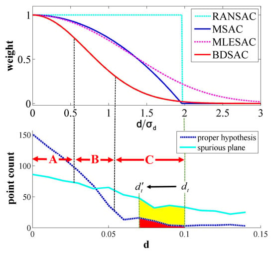
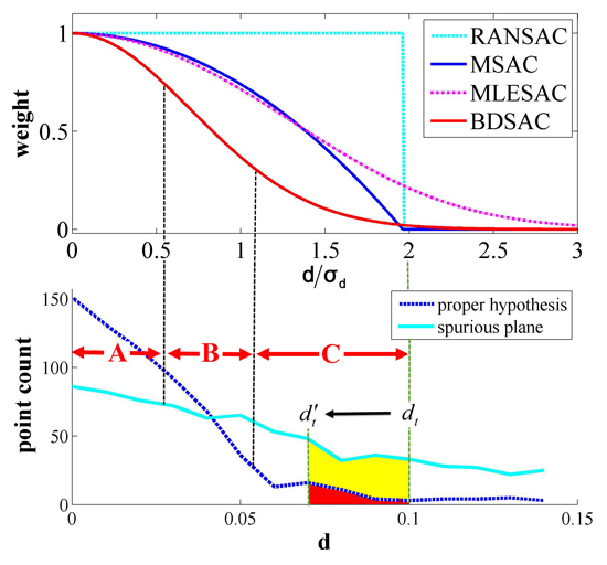
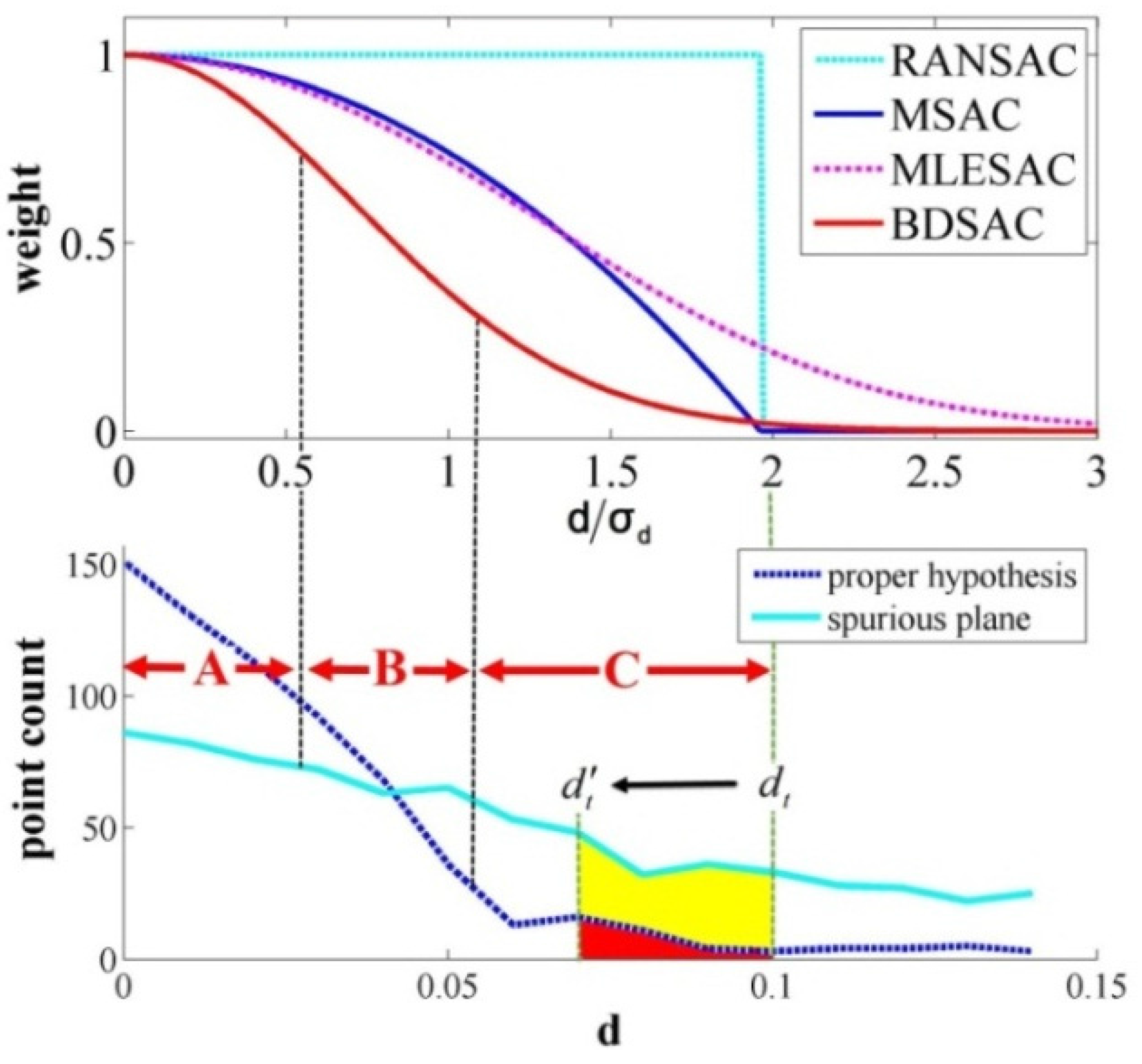
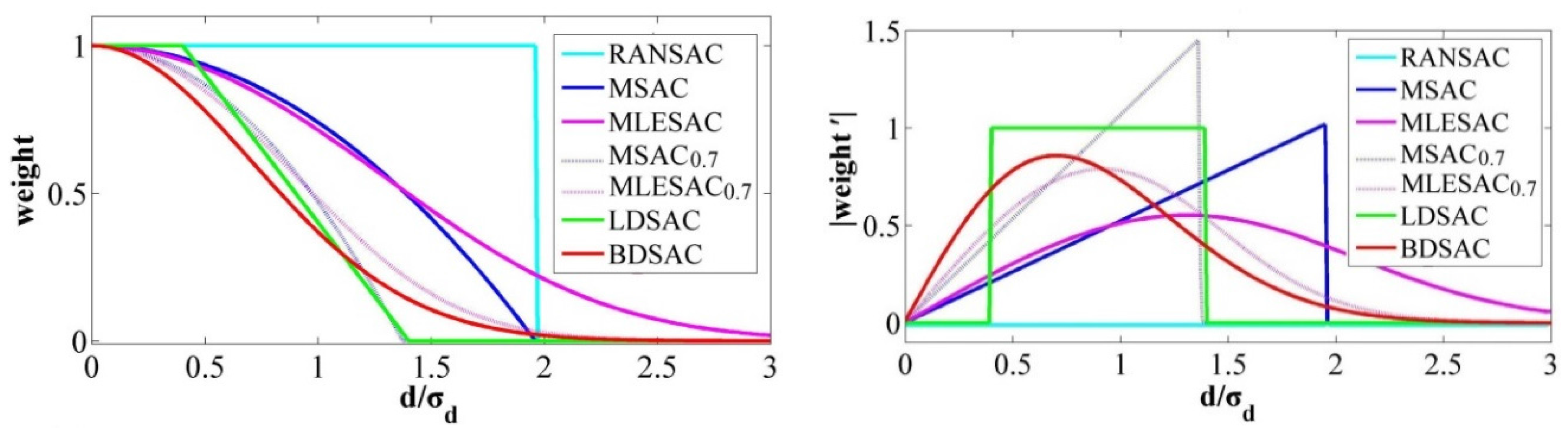
3.1. Improvements Consideration of the Weighted Function

3.2. Modified Weight Functions and New Weight Functions

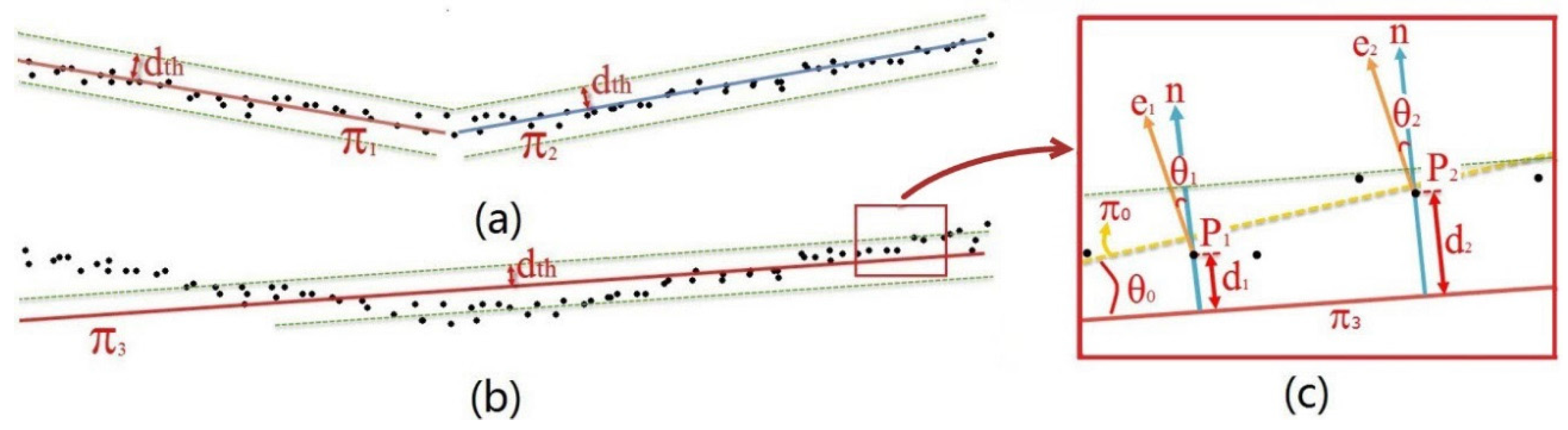
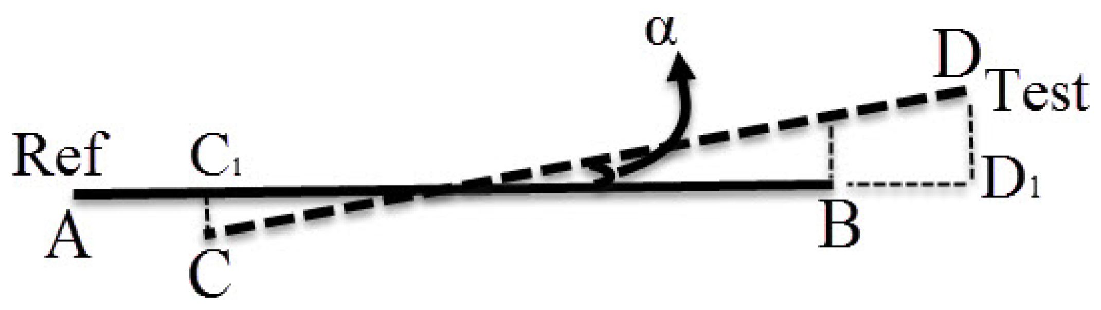
3.3. Joint Weight Function Regarding Angular Difference
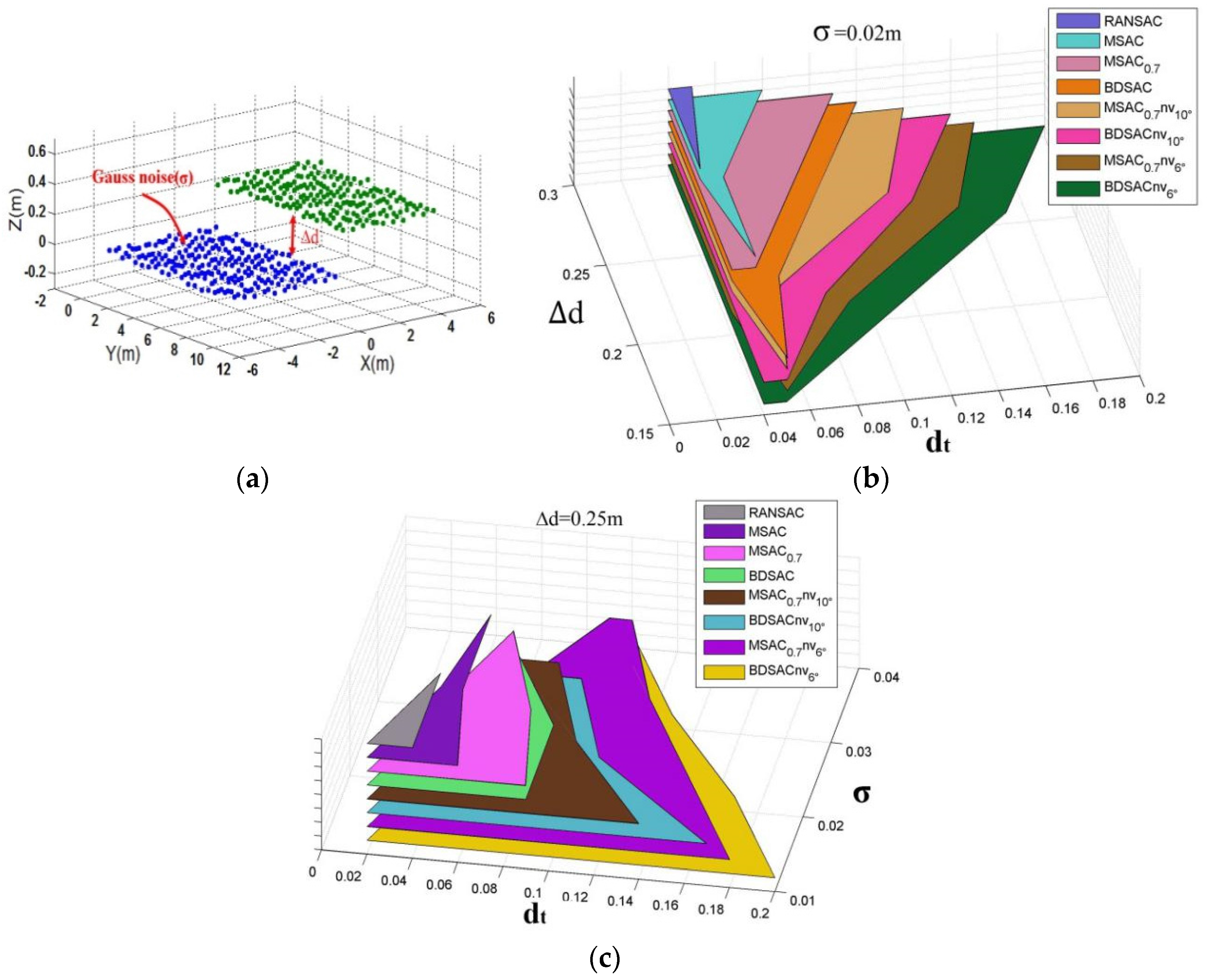
3.4. Weight Function Evaluation
- (1)
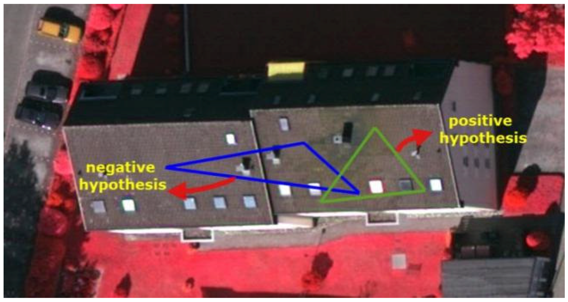
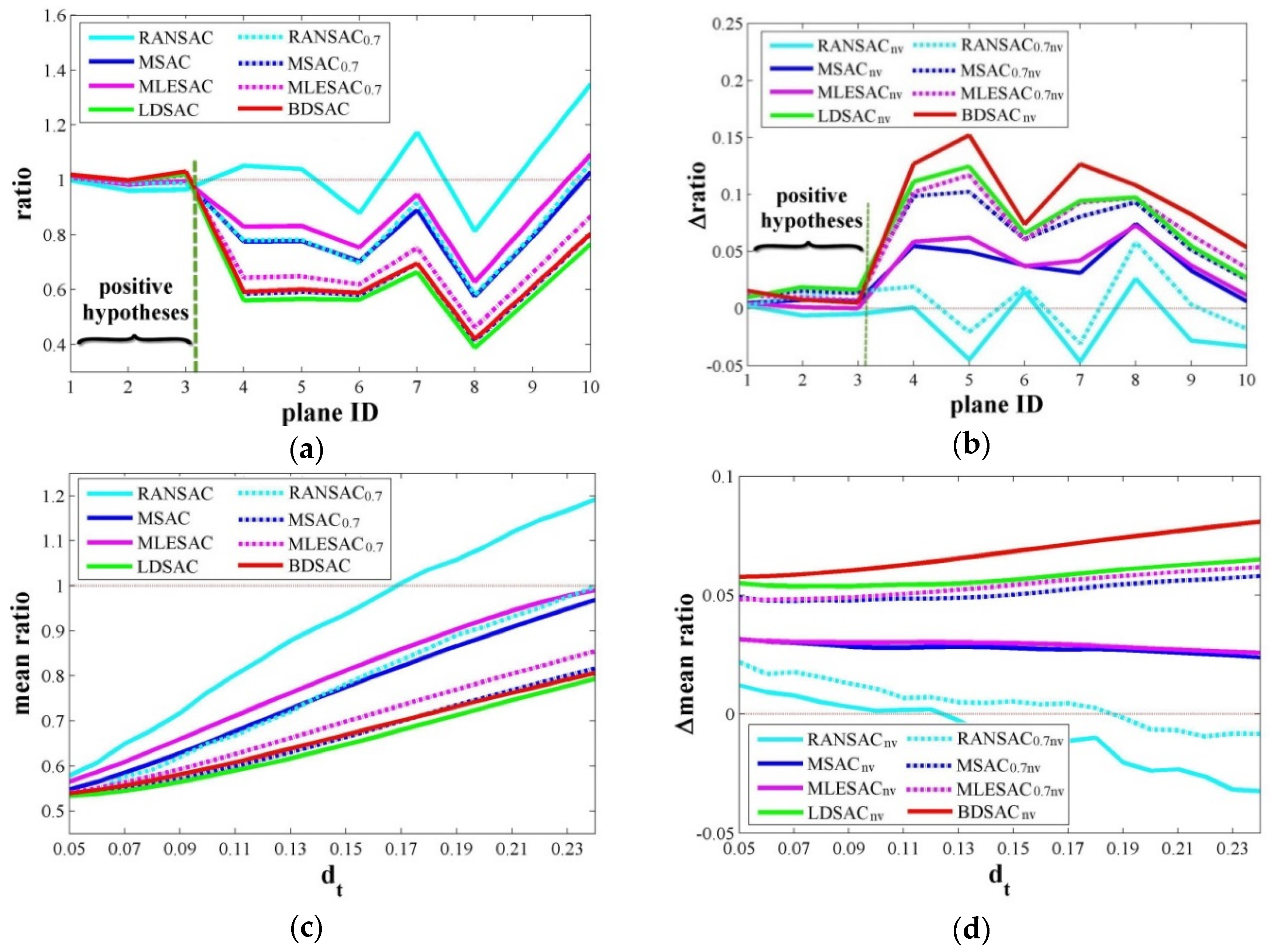
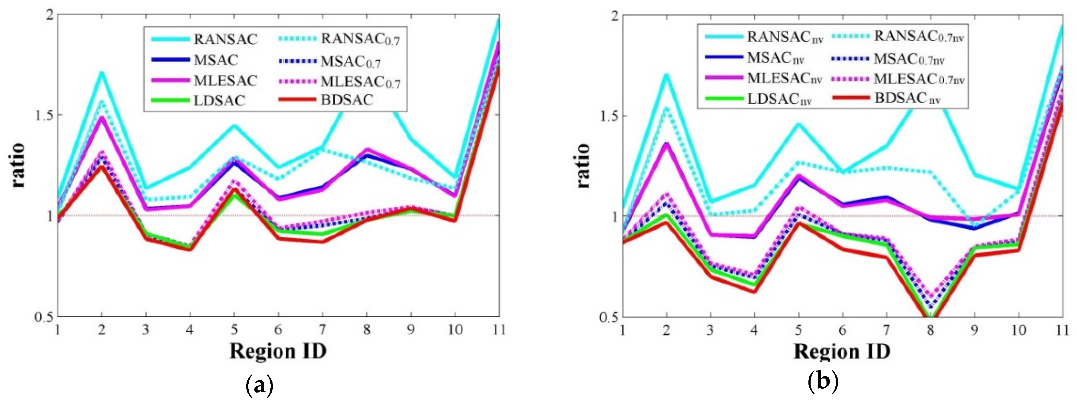
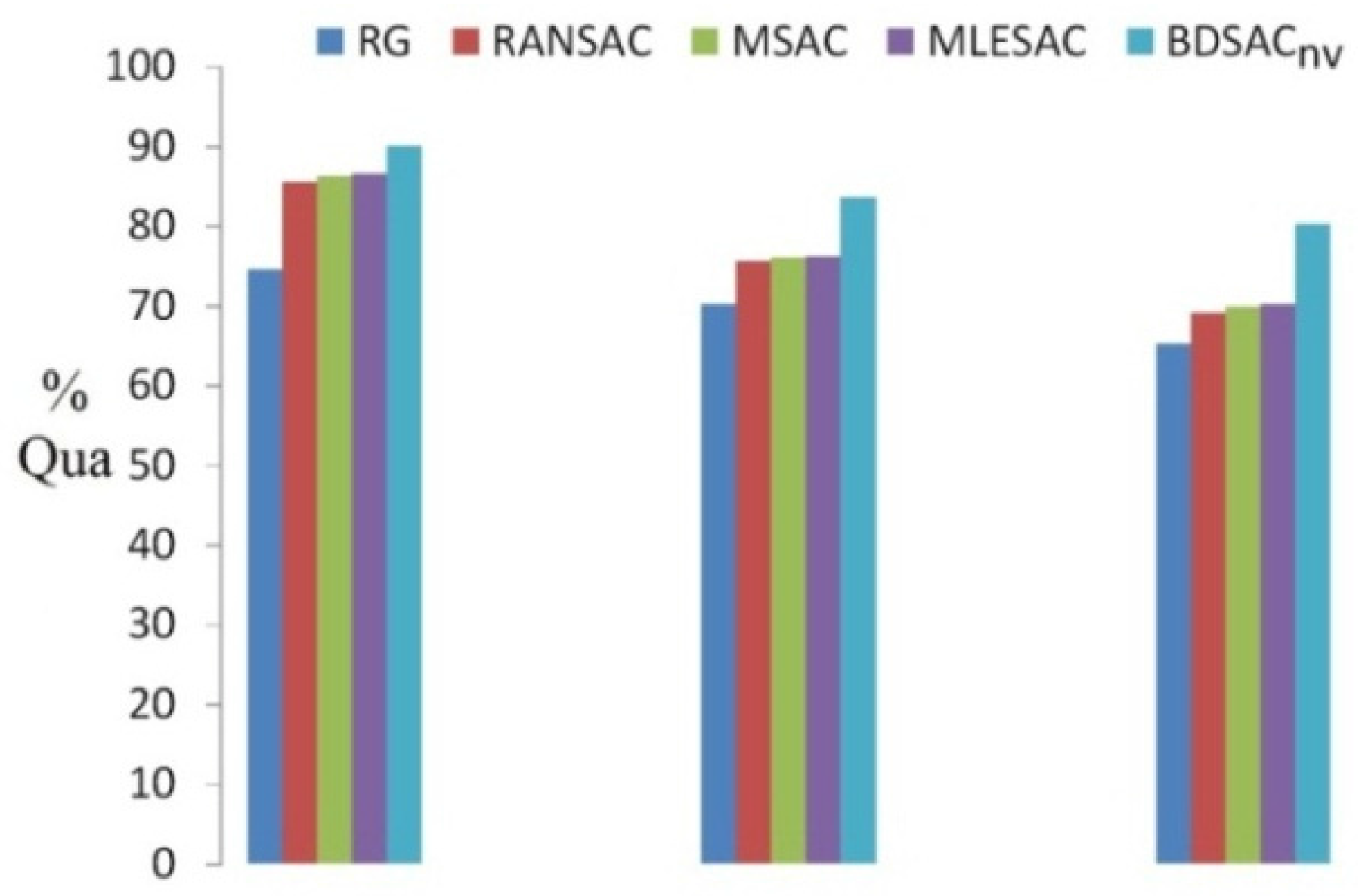
- For all the weighted methods, the evaluation of the positive hypotheses (planes 1, 2, and 3) are stable as the ratios in Figure 5a are close to 1.0 and the ratio reductions in Figure 5b are close to 0. Meanwhile, all the weighted methods can significantly decrease the ratios of the negative hypotheses when compared to RANSAC, but their suppressing ability are different.
- (2)
- By comparing the results between the modified weight functions and the original functions (i.e., MSAC0.7 and MSAC), it can be concluded that reduction of the inlier threshold can suppress the outliers effectively. The newly designed LDSAC and BDSAC functions have the best performances, which verifies our considerations in Section 3.1.
- (3)
- From Figure 5c, it can be seen that all the methods can be affected by the threshold in some degree, but the newly designed weighted methods are least influenced.
- (4)
- Figure 5b,d illustrate the improvements after taking the angular differences into the weight functions. All the weighted methods gain positive effects and the effects are not sensitive to the thresholds.
4. Experiments and Evaluation
4.1. Datasets and Fundamental Algorithm

| Site | Vaihingen | Wuhan |
|---|---|---|
| Acquisition Date | 22 August 2008 | 22 July 2014 |
| Acquisition System | Leica ALS 50 | Trimble Harrier 68i |
| Fly Height | 500 m | 1000 m (cross flight) |
| Point Density | ~4/m2 | >15/m2 |
| MinPt | MinLen | Angle | dt | θt | Ncc | Dcc | P0 | NbPt1 | NbPt2 | |
|---|---|---|---|---|---|---|---|---|---|---|
| Vaihingen | 5 | 1 m | 15° | 0.15 m | 10° | 5 | 1.5 m | 0.99 | 5 | 20 |
| Wuhan | 20 | 1 m | 15° | 0.20 m | 10° | 5 | 0.75 m | 0.99 | 10 | 30 |
4.2. Evaluation Metrics

4.3. Experiments
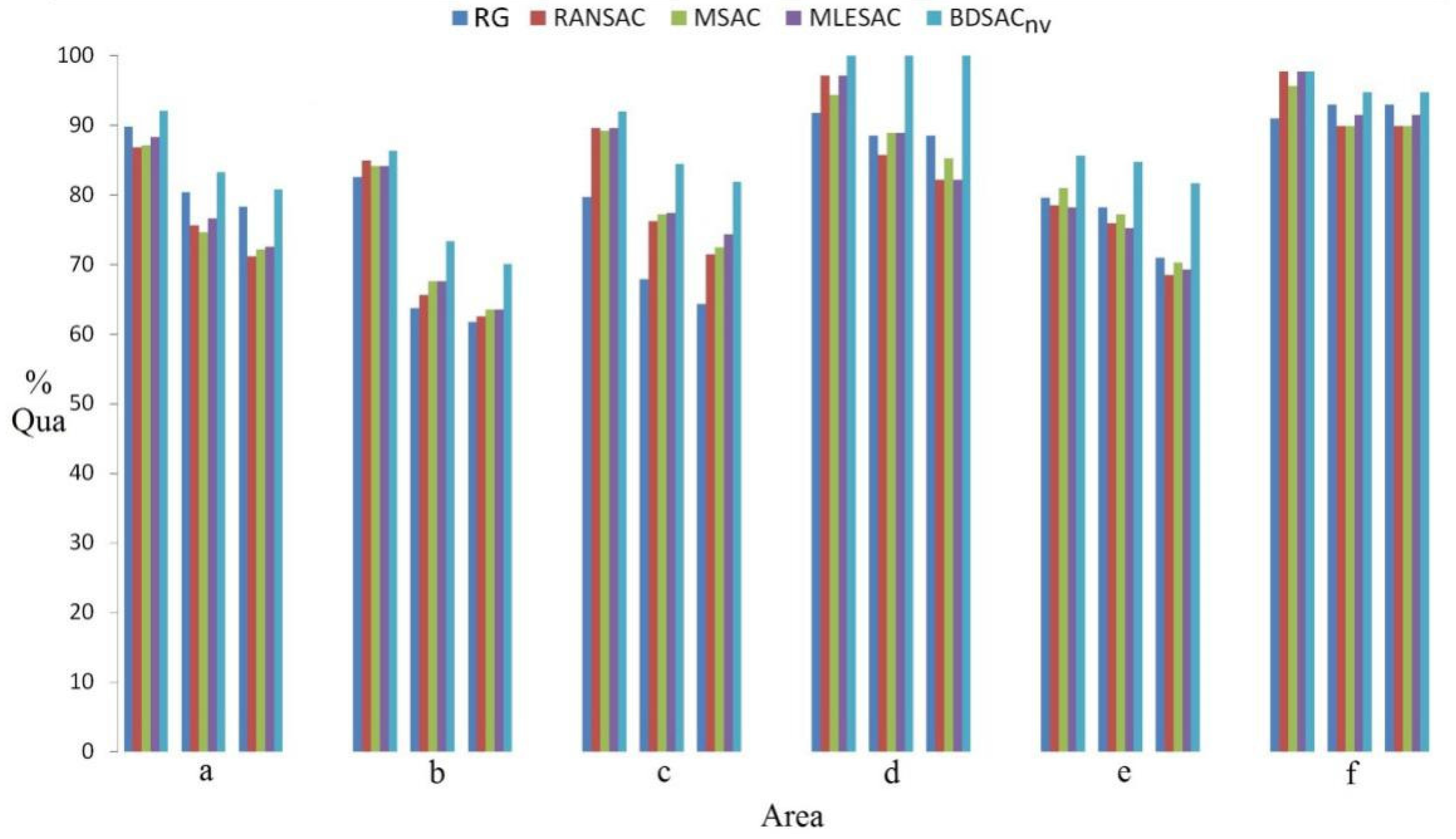
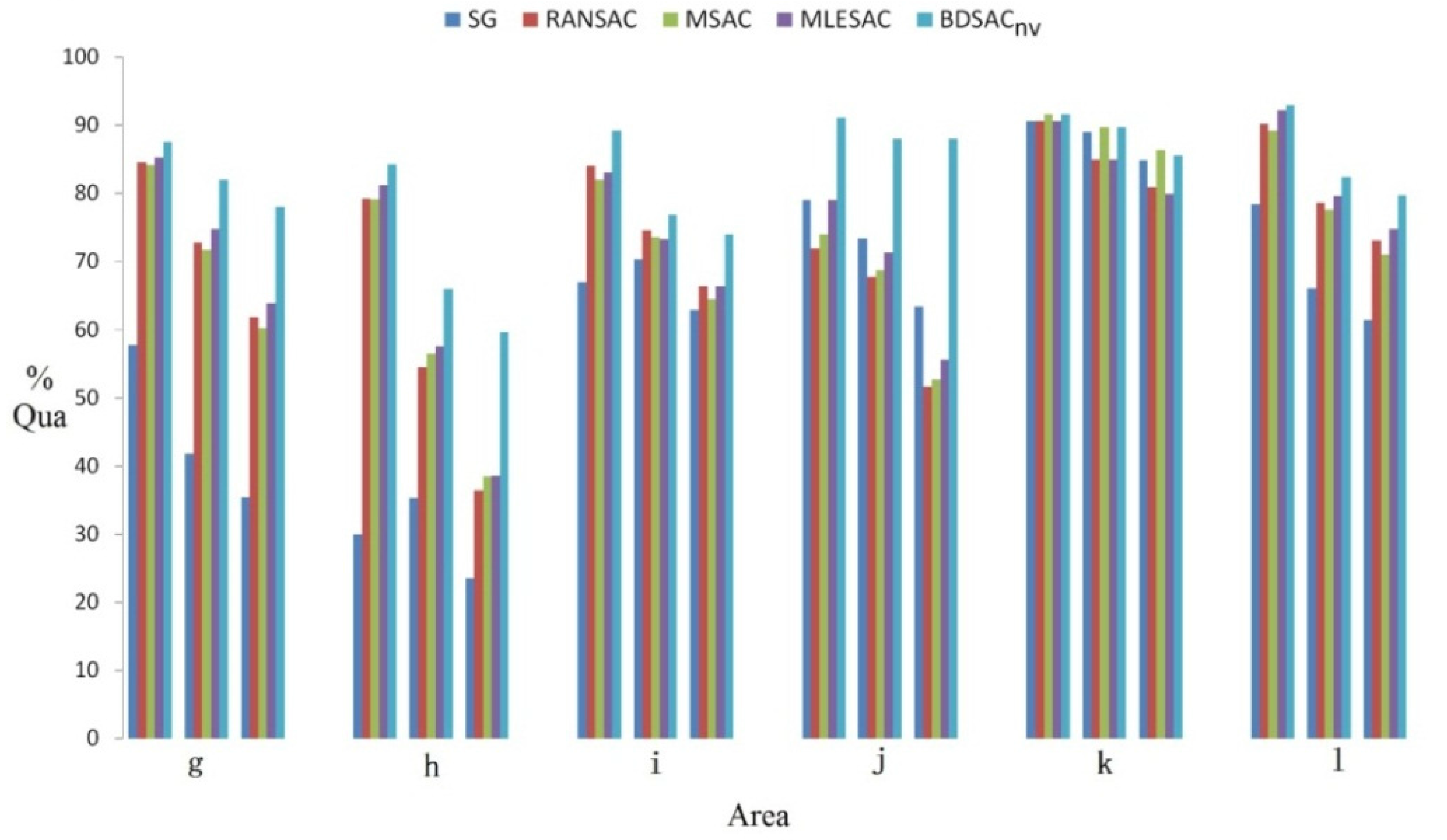
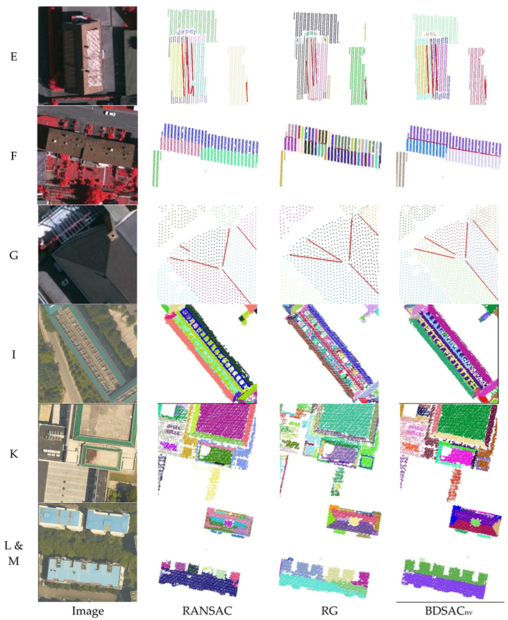
4.3.1. Local Data


| ID | nPls | nRidges | Method | Segmentation | Ridges (RTG) | Ridges (ic > 0.3) | ||||||
|---|---|---|---|---|---|---|---|---|---|---|---|---|
| %Cm | %Cr | %Qua | %Cm | %Cr | %Qua | %Cm | %Cr | %Qua | ||||
| a | 10 | 7 | RANSAC | 80 | 100 | 80 | 71.4 | 55.5 | 45.5 | 57.1 | 44.4 | 33.3 |
| RG | 100 | 100 | 100 | 71.4 | 100 | 71.4 | 71.4 | 100 | 71.4 | |||
| BDSACnv | 100 | 100 | 100 | 100 | 100 | 100 | 71.4 | 100 | 71.4 | |||
| b | 5 | 3 | RANSAC | 80 | 57.1 | 50 | 66.7 | 50.0 | 40.0 | 0 | 0 | 0 |
| RG | 100 | 100 | 100 | 100 | 100 | 100 | 100 | 100 | 100 | |||
| BDSACnv | 100 | 100 | 100 | 100 | 100 | 100 | 100 | 100 | 100 | |||
| c | 7 | 5 | RANSAC | 85.7 | 60 | 51.5 | 60.0 | 37.5 | 30.0 | 40.0 | 25.0 | 18.2 |
| RG | 85.7 | 75 | 66.7 | 100 | 71.4 | 71.4 | 100 | 71.4 | 71.4 | |||
| BDSACnv | 100 | 100 | 100 | 100 | 83.3 | 83.3 | 100 | 83.3 | 83.3 | |||
| d | 10 | 11 | RANSAC | 80.0 | 100 | 80.0 | 90.9 | 100 | 90.9 | 90.9 | 100 | 90.9 |
| RG | 80.0 | 100 | 80.0 | 90.9 | 100 | 90.9 | 90.9 | 100 | 90.9 | |||
| BDSACnv | 100 | 100 | 100 | 100 | 100 | 100 | 100 | 100 | 100 | |||
| e | 9 | 7 | RANSAC | 88.9 | 100 | 88.9 | 71.4 | 100 | 71.4 | 57.1 | 80 | 50 |
| RG | 60 | 100 | 60 | 71.4 | 100 | 71.4 | 57.1 | 80 | 50 | |||
| BDSACnv | 100 | 100 | 100 | 100 | 100 | 100 | 100 | 100 | 100 | |||
| f | 12 | 12 | RANSAC | 66.7 | 66.7 | 50 | 33.3 | 50.0 | 25.0 | 33.3 | 50 | 25.0 |
| RG | 83.3 | 90.9 | 76.9 | 41.7 | 55.5 | 31.2 | 41.7 | 55.5 | 31.2 | |||
| BDSACnv | 91.7 | 91.7 | 84.6 | 91.7 | 91.7 | 84.6 | 66.7 | 66.7 | 50.0 | |||
| g | 23 | 5 | RANSAC | 69.6 | 64.0 | 50.0 | 100 | 62.5 | 62.5 | 100 | 62.5 | 62.5 |
| RG | 78.3 | 72.0 | 60.0 | 100 | 71.4 | 71.4 | 100 | 71.4 | 71.4 | |||
| BDSACnv | 69.6 | 66.7 | 51.6 | 100 | 50.0 | 50.0 | 100 | 50.0 | 50.0 | |||
| h | 11 | 10 | RANSAC | 90.9 | 71.4 | 66.7 | 90.0 | 64.3 | 60.0 | 80.0 | 57.1 | 50.0 |
| RG | 81.8 | 69.2 | 60.0 | 70.0 | 46.7 | 38.9 | 60.0 | 40.0 | 31.6 | |||
| BDSACnv | 90.9 | 66.7 | 62.5 | 90.0 | 69.2 | 64.3 | 80.0 | 61.5 | 53.3 | |||
| sum | 87 | 60 | RANSAC | 78.2 | 73.9 | 61.3 | 71.7 | 65.2 | 51.8 | 61.7 | 56.1 | 41.6 |
| RG | 82.8 | 83.7 | 71.3 | 75.0 | 73.8 | 59.2 | 71.7 | 70.5 | 55.1 | |||
| BDSACnv | 89.7 | 84.8 | 77.2 | 96.7 | 84.1 | 81.7 | 86.7 | 77.6 | 69.3 | |||
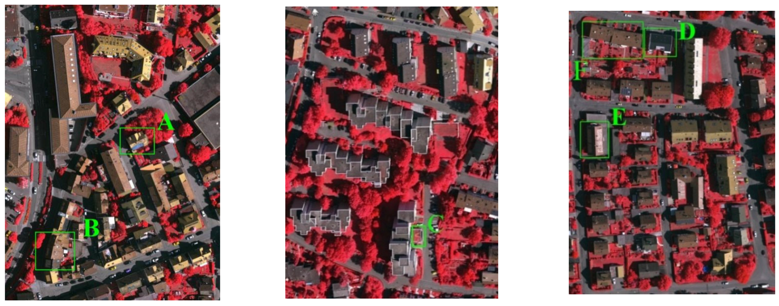
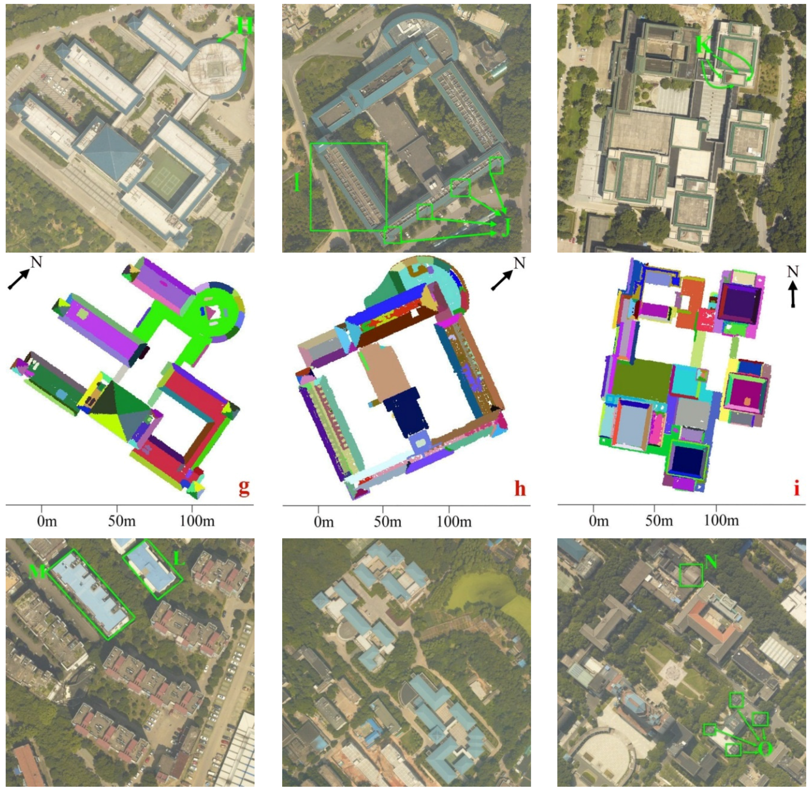
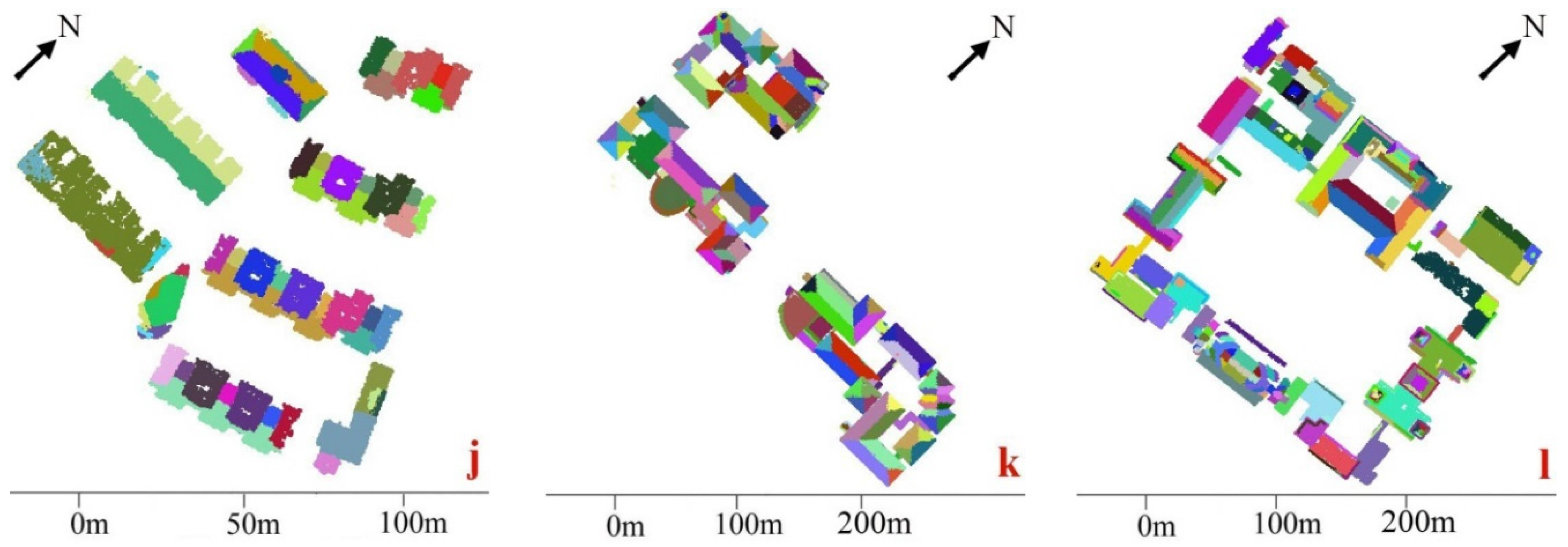
4.3.2. Vaihingen (Germany)

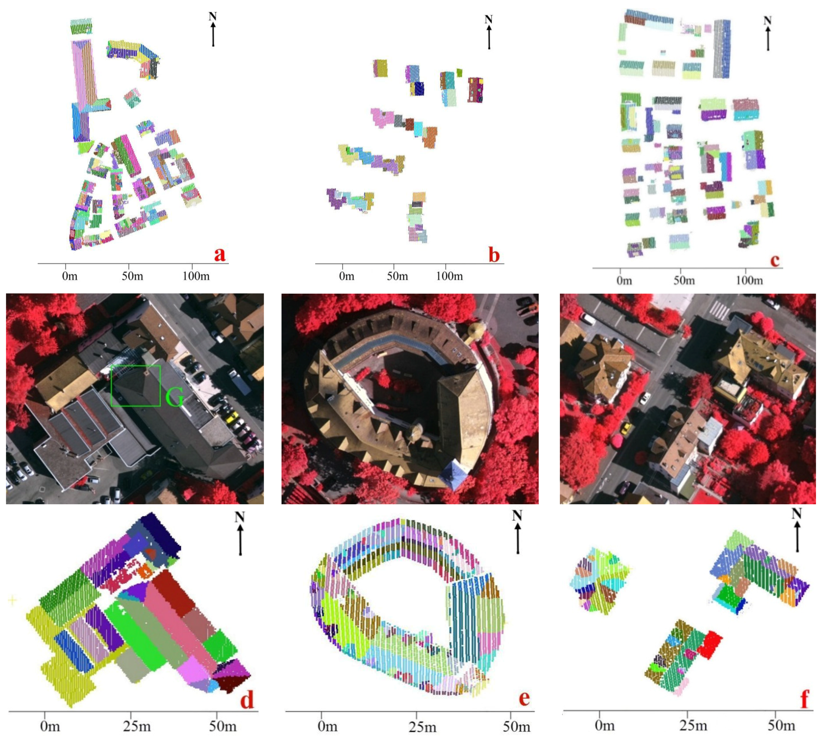

4.3.3. Wuhan University (China)

5. Conclusions
Acknowledgments
Author Contributions
Conflicts of Interest
Appendix I
References
- Baltsavias, E.P. Object extraction and revision by image analysis using existing geodata and knowledge: Current status and steps towards operational systems. ISPRS J. Photogramm. Remote Sens. 2004, 58, 129–151. [Google Scholar] [CrossRef]
- Haala, N.; Kada, M. An update on automatic 3D building reconstruction. ISPRS J. Photogramm. Remote Sens. 2010, 65, 570–580. [Google Scholar] [CrossRef]
- Rottensteiner, F.; Sohn, G.; Gerke, M.; Wegner, J.D.; Breitkopf, U.; Jung, J. Results of the ISPRS benchmark on urban object detection and 3D building reconstruction. ISPRS J. Photogramm. Remote Sens. 2014, 93, 256–271. [Google Scholar] [CrossRef]
- Chen, D.; Zhang, L.Q.; Li, J.; Liu, R. Urban building roof segmentation from airborne Lidar point clouds. Int. J. Remote Sens. 2012, 33, 6497–6515. [Google Scholar] [CrossRef]
- Tarsha-Kurdi, F.; Landes, T.; Grussenmeyer, P.; Koehl, M. Model-driven and data-driven approaches using Lidar data analysis and comparison. In Proceedings of the ISPRS, Workshop, Photogrammetric Image Analysis (PIA07), Munich, Germany, 19–21 September 2007.
- Sampath, A.; Shan, J. Segmentation and reconstruction of polyhedral building roofs from aerial Lidar point clouds. IEEE Trans. Geosci. Remote Sens. 2010, 48, 1554–1567. [Google Scholar] [CrossRef]
- Awwad, T.M.; Zhu, Q.; Du, Z.; Zhang, Y. An improved segmentation approach for planar surfaces from unconstructed 3D point clouds. Photogramm. Rec. 2010, 25, 5–23. [Google Scholar] [CrossRef]
- Fan, T.J.; Medioni, G.; Nevatia, R. Segmented descriptions of 3-D surfaces. IEEE Trans. Rob. Autom. 1987, 3, 527–538. [Google Scholar]
- Alharthy, A.; Bethel, J. Detailed building reconstruction from airborne laser data using a moving surface method. Int. Arch. Photogramm. Remote Sens. 2004, 35, 213–218. [Google Scholar]
- You, R.J.; Lin, B.C. Building feature extraction from airborne Lidar data based on tensor voting algorithm. Photogramm. Eng. Remote Sens. 2011, 77, 1221–1231. [Google Scholar] [CrossRef]
- Vosselman, G. Automated planimetric quality control in high accuracy airborne laser scanning surveys. ISPRS J. Photogramm. Remote Sens. 2012, 74, 90–100. [Google Scholar] [CrossRef]
- Lagüela, S.; Díaz-Vilariño, L.; Armesto, J.; Arias, P. Non-destructive approach for the generation and thermal characterization of an as-built BIM. Constr. Build. Mater. 2014, 51, 55–61. [Google Scholar] [CrossRef]
- Hoffman, R.; Jain, A.K. Segmentation and classification of range images. IEEE Trans. Pattern Anal. Mach. Intell. 1987, 9, 608–620. [Google Scholar] [CrossRef] [PubMed]
- Filin, S. Surface clustering from airborne laser scanning data. Int. Arch. Photogramm. Remote Sens. 2002, 34, 119–124. [Google Scholar]
- Filin, S.; Pfeifer, N. Segmentation of airborne laser scanning data using a slope adaptive neighborhood. ISPRS J. Photogramm. Remote Sens. 2006, 60, 71–80. [Google Scholar] [CrossRef]
- Biosca, J.M.; Lerma, J.L. Unsupervised robust planar segmentation of terrestrial laser scanner point clouds based on fuzzy clustering methods. ISPRS J. Photogramm. Remote Sens. 2008, 63, 84–98. [Google Scholar] [CrossRef]
- Dorninger, P.; Pfeifer, N. A comprehensive automated 3D approach for building extraction, reconstruction, and regularization from airborne laser scanning point clouds. Sensors 2008, 8, 7323–7343. [Google Scholar] [CrossRef]
- Awrangjeb, M.; Fraser, C.S. Automatic segmentation of raw Lidar data for extraction of building roofs. Remote Sens. 2014, 6, 3716–3751. [Google Scholar] [CrossRef]
- Fischler, M.A.; Bolles, R.C. Random sample consensus—A paradigm for model-fitting with applications to image-analysis and automated cartography. Commun. ACM 1981, 24, 381–395. [Google Scholar] [CrossRef]
- Schnabel, R.; Wahl, R.; Klein, R. Efficient RANSAC for point-cloud shape detection. Comput. Graph. Forum 2007, 26, 214–226. [Google Scholar] [CrossRef]
- Choi, S.; Kim, T.; Yu, W. Performance evaluation of RANSAC family. In Proceedings of the British Machine Vision Conference, London, UK, 7–10 September 2009.
- Frahm, J.-M.; Pollefeys, M. RANSAC for (Quasi-) degenerate data (QDEGSAC). In Proceedings of the IEEE Computer Society Conference on Computer Vision and Pattern Recognition, New York, NY, USA, 17–22 June 2006.
- Chum, O.R.; Matas, J.R.I. Matching with PROSAC-progressive sampling consensus. In Proceedings of the IEEE Computer Society Conference on Computer Vision and Pattern Recognition, Miami, FL, USA, 20–25 June 2005.
- Chum, O.; Matas, J. Optimal randomized RANSAC. IEEE Trans. Pattern Anal. Mach. Intell. 2008, 30, 1472–1482. [Google Scholar] [CrossRef] [PubMed]
- Berkhin, P. A Survey of Clustering Data Mining Techniques; Springer Berlin Heidelberg: New York, NY, USA, 2006. [Google Scholar]
- Gallo, O.; Manduchi, R.; Rafii, A. CC-RANSAC: Fitting planes in the presence of multiple surfaces in range data. Pattern Recognit. Lett. 2011, 32, 403–410. [Google Scholar] [CrossRef]
- Yan, J.X.; Shan, J.; Jiang, W.S. A global optimization approach to roof segmentation from airborne Lidar point clouds. ISPRS J. Photogramm. Remote Sens. 2014, 94, 183–193. [Google Scholar] [CrossRef]
- Xiong, B.; Elberink, S.O.; Vosselman, G. A graph edit dictionary for correcting errors in roof topology graphs reconstructed from point clouds. ISPRS J. Photogramm. Remote Sens. 2014, 93, 227–242. [Google Scholar] [CrossRef]
- Elberink, S.O.; Vosselman, G. Building reconstruction by target based graph matching on incomplete laser data: Analysis and limitations. Sensors 2009, 9, 6101–6118. [Google Scholar] [CrossRef] [PubMed]
- Hesami, R.; BabHadiashar, A.; HosseinNezhad, R. Range segmentation of large building exteriors: A hierarchical robust approach. Comput. Vis. Image Underst. 2010, 114, 475–490. [Google Scholar] [CrossRef]
- Torr, P.H.S.; Zisserman, A. Mlesac: A new robust estimator with application to estimating image geometry. Comput. Vis. Image Underst. 2000, 78, 138–156. [Google Scholar] [CrossRef]
- Bretar, F.; Roux, M. Hybrid image segmentation using Lidar 3D planar primitives. In Proceedings of the ISPRS Workshop Laser Scanning, Enschede, The Netherlands, 12–14 September 2005.
- López-Fernández, L.; Lagüela, S.; Picón, I.; González-Aguilera, D. Large-scale automatic analysis and classification of roof surfaces for the installation of solar panels using a multi-sensor aerial platform. Remote Sens. 2015, 7, 11226–11248. [Google Scholar] [CrossRef]
- Wang, C.; Sha, Y. A designed beta-hairpin forming peptide undergoes a consecutive stepwise process for self-assembly into nanofibrils. Protein Pept. Lett. 2010, 17, 410–415. [Google Scholar] [CrossRef] [PubMed]
- Girardeau-Montaut, D. Detection de Changement sur des Données Géométriques 3D. Ph.D. Thesis, Télécom ParisTech, Paris, France, 2006. [Google Scholar]
- Awrangjeb, M.; Fraser, C.S. An automatic and threshold-free performance evaluation system for building extraction techniques from airborne Lidar data. IEEE J. Sel. Top. Appl. Earth Observ. Remote Sens. 2014, 7, 4184–4198. [Google Scholar] [CrossRef]
- Rutzinger, M.; Rottensteiner, F.; Pfeifer, N. A comparison of evaluation techniques for building extraction from airborne laser scanning. IEEE J. Sel. Top. Appl. Earth Observ. Remote Sens. 2009, 2, 11–20. [Google Scholar] [CrossRef]
- Perera, G.S.N.; Maas, H.G. Cycle graph analysis for 3D roof structure modeling: Concepts and performance. ISPRS J. Photogramm. Remote Sens. 2014, 93, 213–226. [Google Scholar] [CrossRef]
© 2015 by the authors; licensee MDPI, Basel, Switzerland. This article is an open access article distributed under the terms and conditions of the Creative Commons by Attribution (CC-BY) license (http://creativecommons.org/licenses/by/4.0/).
Share and Cite
Xu, B.; Jiang, W.; Shan, J.; Zhang, J.; Li, L. Investigation on the Weighted RANSAC Approaches for Building Roof Plane Segmentation from LiDAR Point Clouds. Remote Sens. 2016, 8, 5. https://doi.org/10.3390/rs8010005
Xu B, Jiang W, Shan J, Zhang J, Li L. Investigation on the Weighted RANSAC Approaches for Building Roof Plane Segmentation from LiDAR Point Clouds. Remote Sensing. 2016; 8(1):5. https://doi.org/10.3390/rs8010005
Chicago/Turabian StyleXu, Bo, Wanshou Jiang, Jie Shan, Jing Zhang, and Lelin Li. 2016. "Investigation on the Weighted RANSAC Approaches for Building Roof Plane Segmentation from LiDAR Point Clouds" Remote Sensing 8, no. 1: 5. https://doi.org/10.3390/rs8010005
APA StyleXu, B., Jiang, W., Shan, J., Zhang, J., & Li, L. (2016). Investigation on the Weighted RANSAC Approaches for Building Roof Plane Segmentation from LiDAR Point Clouds. Remote Sensing, 8(1), 5. https://doi.org/10.3390/rs8010005