1. Introduction
Synthetic Aperture Radar (SAR) Interferometry (InSAR) is a well-known technique that allows the generation of the Digital Elevation Model (DEM) of an area through the exploitation of the phase difference (interferogram) between SAR data pairs relevant to the same observed scene and received from slightly different view angles [
1,
2].
SAR sensors can be mounted on satellites, space-shuttles, airplanes, helicopters and ground stations. In the former case, the images and the corresponding interferometric products are characterized by a wider spatial coverage coupled to a geometric resolution typically lower than that achievable in the other cases, where smaller antennas can be exploited [
1]. In all the cases, the InSAR configurations can be obtained either by means of repeated passes of the sensor over the same area or by exploiting multiple antennas forming a single-pass system [
1].
As for the spaceborne systems, the generation of InSAR products is a relatively assessed task, due to the high stability of the orbits covered by the platforms. Indeed, this kind of acquisition geometry simplifies the SAR focusing step and the subsequent InSAR processing chain [
1]. With particular reference to the DEM generation, the temporal decorrelation effects [
1] may be very severe in repeat-pass spaceborne acquisitions; single-pass systems are therefore preferred. For instance, the worldwide SRTM DEM has been obtained through a space shuttle mission that exploited a single-pass configuration [
3]. Moreover, the current TanDEM-X mission [
4] exploits two satellite platforms to form a single-pass configuration aimed at obtaining a worldwide product with resolution higher than that of the SRTM DEM.
Turning to the airborne systems, in principle all of them allow carrying out repeat-pass InSAR. Indeed, due to the operational flexibility peculiar to the airborne platforms, the revisit time between two repeated passes can be kept very short, thus strongly limiting the decorrelation effects typical of spaceborne repeat-pass systems. However, differently from the spaceborne case, the generation of repeat-pass airborne InSAR products is not a turn of the crank procedure. This is due to the platform deviations from a rectilinear, reference flight track. Indeed, such track deviations, which are induced by atmospheric turbulences and winds, produce on the received data so called motion errors [
5], which need to be properly compensated. To this aim, proper algorithms implementing the so called Motion Compensation (MOCO) [
6,
7] procedure must be applied. In particular, their implementation requires the knowledge of the sensor positions during the acquisition and the availability of an external DEM of the observed area. Accordingly, the effectiveness of such MOCO algorithms can be impaired on one hand by the limited precision of the navigation unit mounted on board, and on the other hand by the inaccuracy of the available external DEM [
5]. In addition, in order to efficiently account for the space-variant nature of the motion errors, some approximations are usually applied during the MOCO procedure [
8]. For these reasons, the focused airborne SAR data are typically affected by the so called residual motion errors [
5], not compensated by the MOCO procedure. In particular, the most critical residual motion errors are those induced by the navigation unit inaccuracies [
9]. To this regard, it must be underlined that such errors become less critical in single-pass InSAR systems, since they are quite similar in the different interferometric channels and therefore tend to cancel each other during the InSAR pair beating. Differently, in the repeat-pass airborne InSAR systems, the residual MOCO errors may severely impair the accuracy of the final interferograms, especially when high frequency systems (namely, operating from C- to Ka-bands) are employed. For these reasons, airborne repeat-pass InSAR DEMs are typically generated with low frequency systems, such as the P-Band OrbiSAR one [
10], which employ wavelengths that are quite large if compared with the typical positioning errors of the modern navigation units. To this regard, it is also stressed that low frequency systems may hardly work in a single-pass airborne configuration. Indeed, to keep the height of ambiguity [
2] of the interferometric configuration sufficiently low, the appropriate InSAR baseline would be too large with respect to the fuselage of airplanes typically exploited for SAR missions. Notwithstanding, some examples of single-pass airborne systems operating at low frequencies exist (consider for instance the P-Band GeoSAR [
11]).
More generally, single-pass airborne InSAR systems typically exploit higher frequencies. Examples of such systems are the C-/X-Band F-SAR [
12], the X-Band PAMIR [
13], the X-/Ku-Band RAMSES [
14], the X-Band SETHI [
15], the X-Band OrbiSAR [
9] and the Ka-Band MEMPHIS [
16,
17,
18,
19,
20]. As a matter of fact, in these systems the InSAR baseline can be as small as required by the geometrical constraints imposed by small airborne platforms. As observed above, in such single-pass systems, the residual motion errors affecting the focused data are typically not negligible at the employed frequencies; however, they tend to cancel each other in the corresponding interferograms.
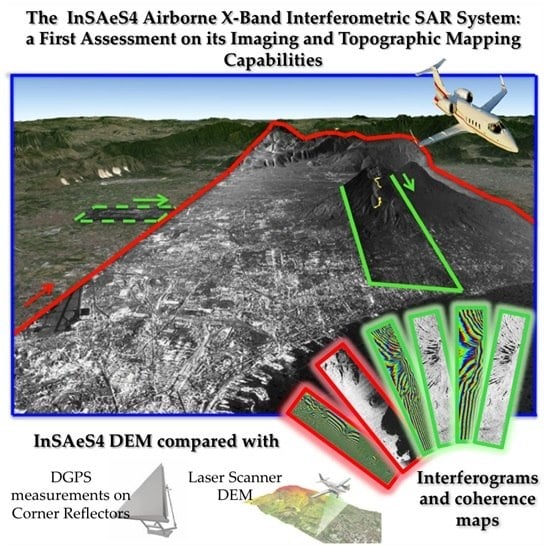
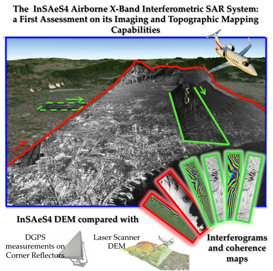
In this work, we present a first assessment of the imaging and topographic mapping capabilities of the X-Band InSAeS4, which is an Italian single-pass interferometric airborne SAR system. More specifically, the InSAeS4, also named TELAER [
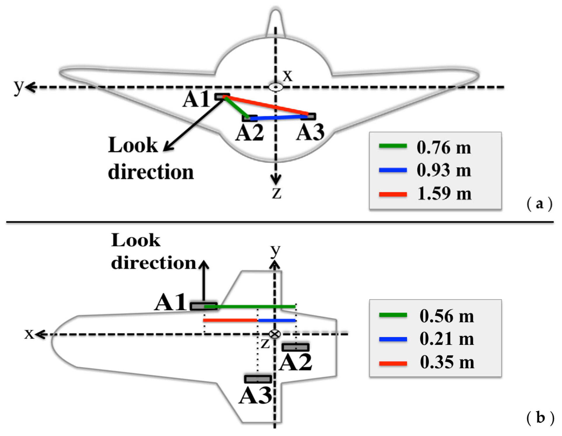
21], is owned by the Italian Agency for Agriculture Subsidy Payments (AGEA) and upgrades the AeS4 system, which was equipped with a single antenna. More specifically, the original AeS4 system has been upgraded to a single-pass interferometric configuration thanks to a funding of the Italian Ministry of Education, Universities and Research (MIUR), through the Italian National Research Council (CNR), in the frame of a cooperation between CNR and AGEA. The system upgrade has been developed by the Institute for the Electromagnetic Sensing of the Environment (IREA), of CNR, and implemented by Orbisat (now Bradar). Thanks to this upgrade, the InSAeS4 system is now equipped with an interferometric layout consisting of three antennas installed in order to allow the simultaneous presence of three Across-Track (XT) baselines for the generation of DEMs [
1,
2], and three Along-Track (AT) baselines mainly for sea surface velocity measurements.
In this work we first provide a description of the InSAeS4 system. Then, we present the results relevant to the acquisition campaign carried out in 2013 just after the ending of the system upgrade. Our analysis is aimed at presenting a first assessment of the imaging and topographic mapping capabilities of the InSAeS4 sensor, in order to provide reference values for future research activities involving the use of the data acquired by this sensor. In particular, we first investigate the imaging capability of the focused data. Then, we concentrate on the characteristics of the single-pass XT InSAR products and present a quantitative assessment of the accuracy of the generated single-pass DEM. To this aim, we provide comparisons with both Differential GPS (DGPS) measurements on Corner Reflectors (CRs) and a laser scanner DEM.
3. Experimental Results
In this Section we present the results relevant to the first flight campaign carried out with the InSAeS4 system over the Napoli area, Italy, in January 2013, just after the completion of the interferometric system upgrade discussed above. In particular, amongst all the settable operational modes, we focus on the full-resolution acquisition mode (400 MHz), for which the system has been designed. Moreover, we also analyze the low-resolution acquisition mode (50 MHz). As shown in
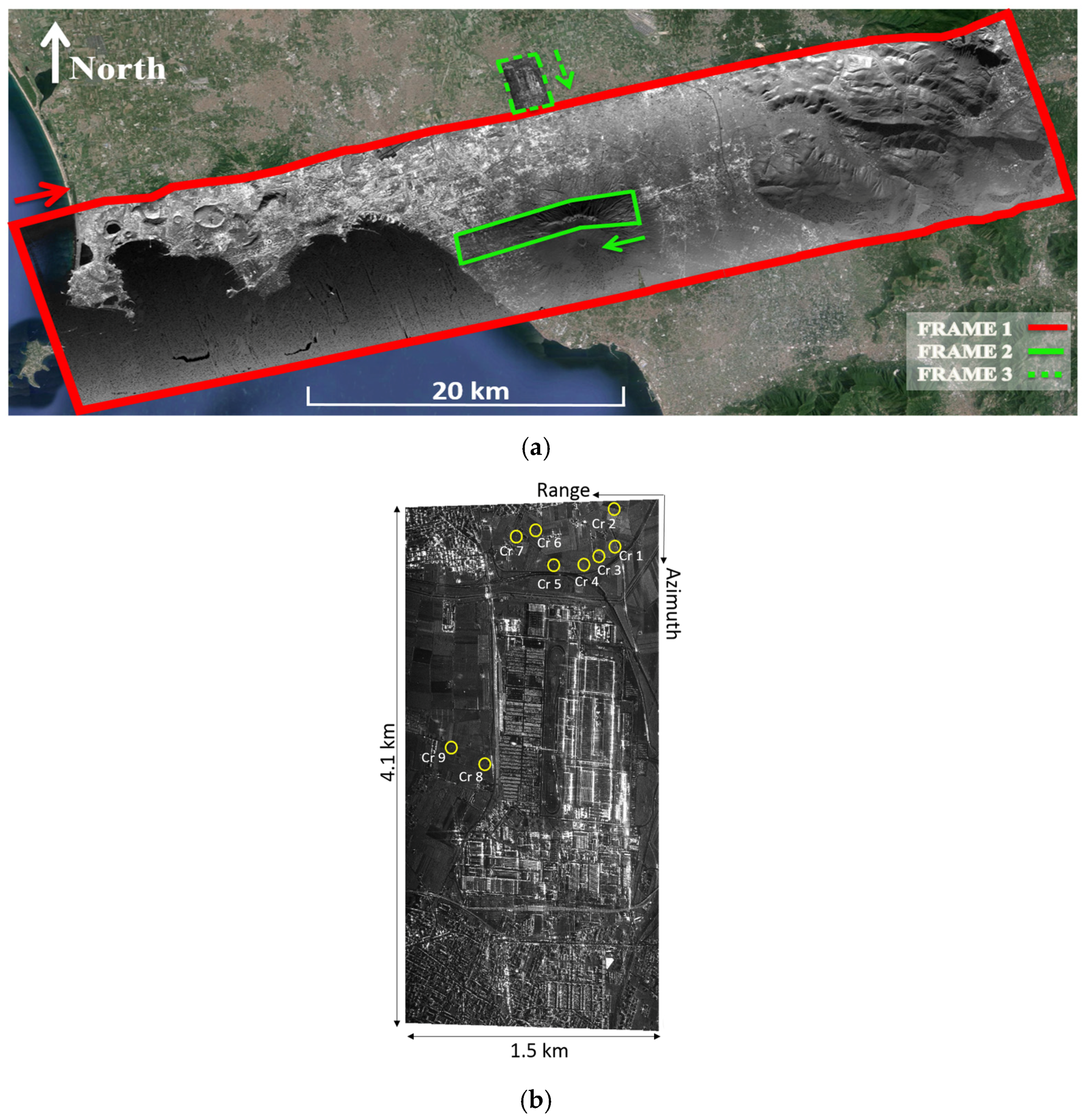
Figure 3a, we consider the three acquisitions (whose main parameters are summarized in
Table 5) relevant to the Campi Flegrei Caldera area and the Somma-Vesuvio volcanic complex.
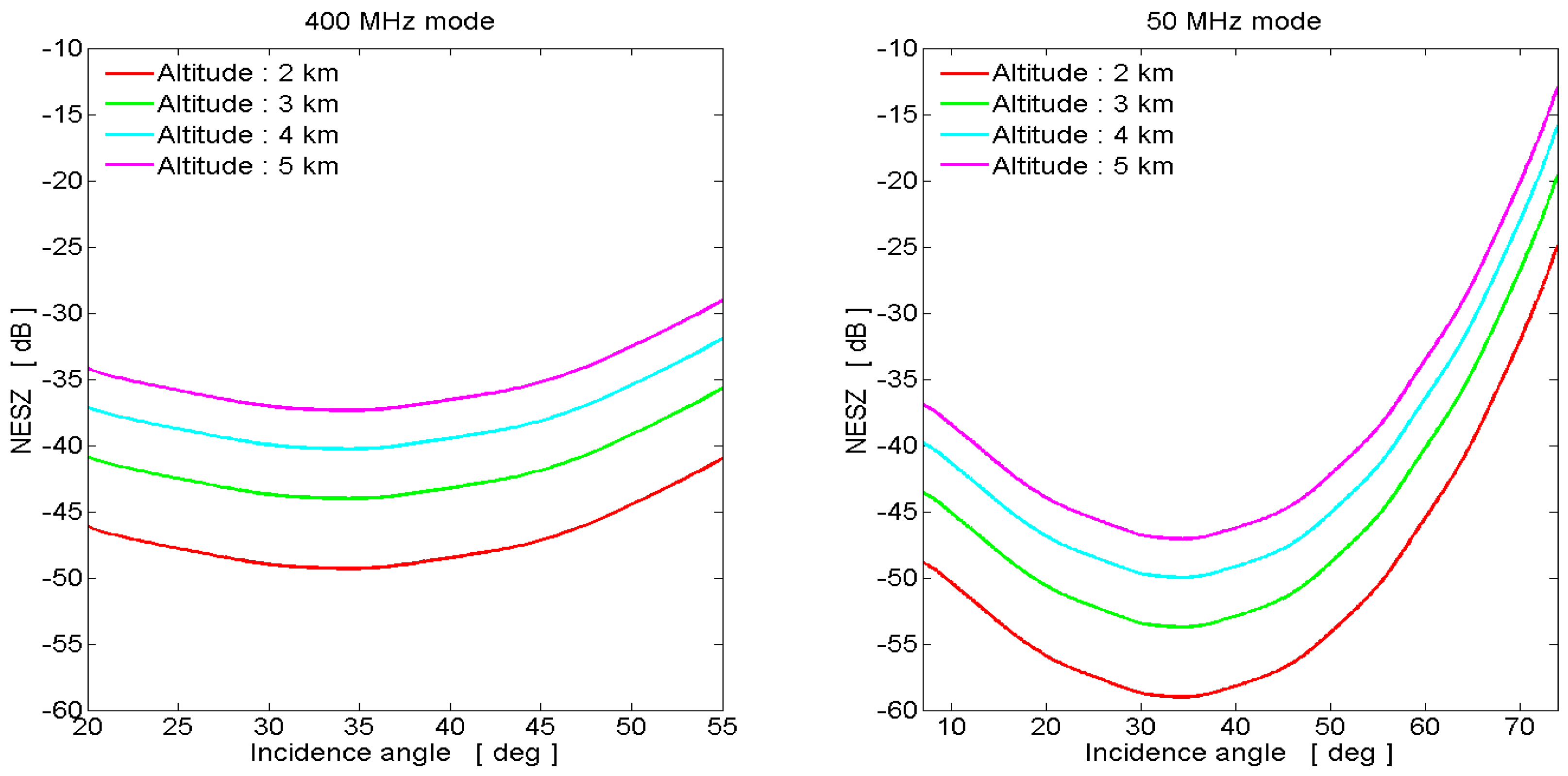
The frame 1 has been acquired with the 50 MHz mode with a single-baseline configuration obtained by activating only the two antennas separated by the largest XT baseline. The flight track is about 65 km long. In this case a 12 km (slant) range swath has been recorded with an off-nadir angle of 30°, which has led to a look angle of about 74° at far range. However, for this acquisition geometry, according to the NESZ curves of
Figure 1 and the analysis of
Section 2, we expect that only a part (corresponding approximately to the angular sector 30°–60°) of the recorded swath can be effectively exploited.
The frames 2 and 3 have been acquired with the 400 MHz mode by exploiting the multi-baseline configuration (that is, all the three antennas activated). In both cases, a 1.5 km (slant) range swath has been recorded with an off-nadir angle of 30°. The flight tracks are about 12 km and 4 km long, respectively. Note that the frame 3 is very short and covers an area where, for calibration purposes, we have deployed 9 CRs and carried out DGPS measurements of their positions.
To process the data we have applied a standard SAR focusing [
1] including the efficient two-step MOCO approach [
6,
7]. In particular, the MOCO corrections have been calculated by exploiting the SRTM external DEM. More specifically, to limit the effects induced by the beam-center approximation [
8] we have applied a 600 m × 400 m smoothing window to the SRTM data before calculating the MOCO corrections.
Figure 3.
(a) Multi-look amplitude SAR images relevant to the acquired data. The frame n.1 (red) is relevant to the 50 MHz mode; the frame n.2 (continuous green) and the frame n.3 (dashed green) are relevant to the 400 MHz mode. The images are geocoded on a 5 × 5 m (50 MHz mode) and 1 × 1 m (400 MHz mode) geographic grid, and superimposed on a Google Earth image. The green and red arrows indicate the flight directions; (b) Amplitude SAR image (in the SAR coordinates grid) relevant to the frame n.3. A 4 range × 16 azimuth pixel averaging window has been applied, obtaining a 1.5 m × 1.85 m pixel spacing. The CRs deployed over the area are highlighted with yellow circles.
Table 5.
SAR acquisitions.
Table 5.
SAR acquisitions.
| | Frame 1 | Frame 2 | Frame 3 |
|---|
| Bandwidth | 50 MHz | 400 MHz | 400 MHz |
| Chirp pulses | 1 | 4 | 4 |
| Pulse duration | 16.2 µs | 2.6 µs | 2.6 µs |
| Azimuth pixel spacing * | 0.08 m | 0.09 m | 0.11 m |
| Azimuth resolution † | 0.12 m | 0.12 m | 0.12 m |
| Range pixel spacing * | 2.99 m | 0.37 m | 0.37 m |
| Range resolution † | 3.84 m | 0.48 m | 0.48 m |
| Range lines | 4096 | 4096 | 4096 |
| Flight altitude | 5001 m | 3962 m | 3962 m |
| Mean platform velocity | 139 m/s | 103 m/s | 126 m/s |
| Look angle | 30°–74° | 30°–50° | 30°–50° |
In the 50 MHz case, we have also applied a 2 azimuth pixel presumming on the raw data [
25]. Finally, we have applied a standard InSAR processing chain. In particular, to coregister the images we have applied a geometric approach [
26] by exploiting again the SRTM external DEM.
In
Figure 3a, the multi-look amplitude SAR images relevant to the three considered acquisitions have been geocoded [
1] and superimposed to a Google Earth image. Note in particular that the 50 MHz and 400 MHz images have been reported on a 5 × 5 m and 1 × 1 m geographic grid, respectively.
Figure 3a clearly shows the different peculiarities of the 400 MHz and the 50 MHz modes. The price paid to achieve the highest resolution is the reduction of the recorded range swath. With particular reference to the high resolution mode,
Figure 3b reports also the SAR image (in the SAR coordinates grid) relevant to the frame 3, with the positions of the CRs highlighted. Note that the CRs are located at different range coordinates, covering the whole illuminated swath.
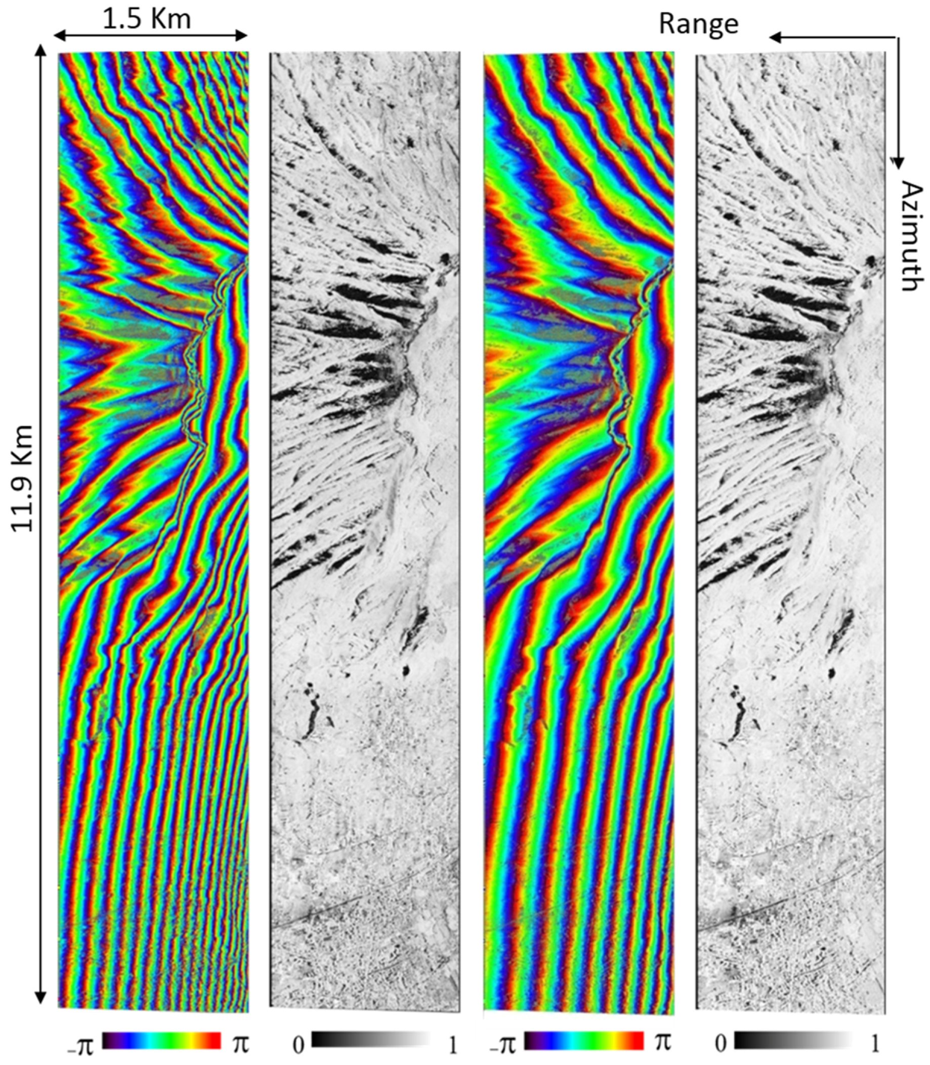
Turning to the InSAR products,
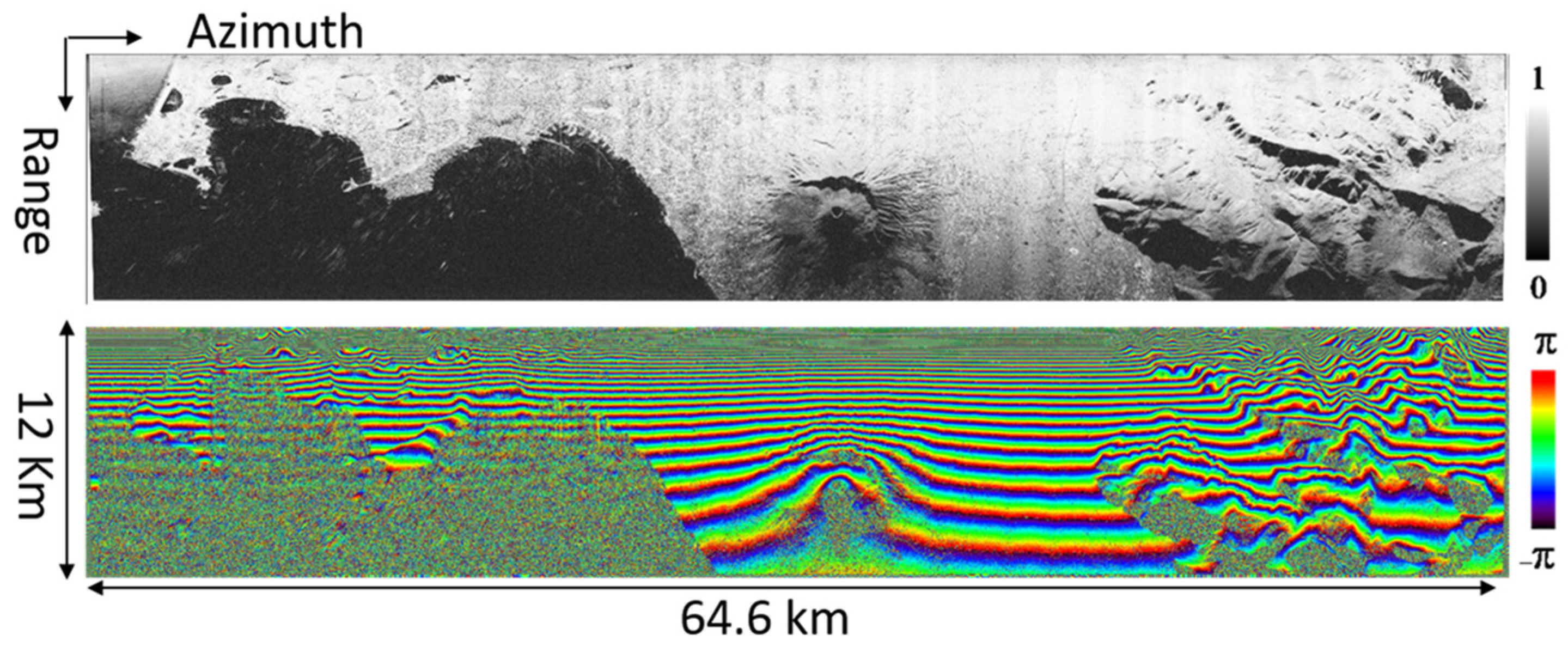
Figure 4 shows, in the SAR coordinates grid, the interferogram and the coherence map relevant to the frame 1. In particular, a simple 24 azimuth pixel averaging has been applied to the interferogram just for visualization purposes (we have indeed obtained an almost square pixel of dimensions equal to 3 m × 4.18 m), without further application of phase noise filters, such as that in [
27].
Figure 4.
Coherence map and interferogram relevant to the frame 1 of
Figure 3a (50 MHz mode, single-baseline configuration). The applied pixel averaging is described in the body of the paper.
Figure 4.
Coherence map and interferogram relevant to the frame 1 of
Figure 3a (50 MHz mode, single-baseline configuration). The applied pixel averaging is described in the body of the paper.
From the top panel of
Figure 4 it can be seen a coherence degradation in far range. In particular, we have measured a fast impairment of the mean coherence for incidence angles greater than approximately 60°. This is in agreement with the NESZ curves of
Figure 1 and confirms that, as expected, only a part (corresponding approximately to the angular sector 30°–60°) of the recorded swath can be effectively exploited with the 50 MHz mode.
As for the full resolution mode,
Figure 5 shows, in the SAR coordinates grid, two coherence maps and two interferograms relevant to the frame 2. In particular, we have considered the two data pairs with the largest (left panels) and the smallest (right panels) XT baselines. Again, we have just applied a simple pixel averaging window (2 range × 12 azimuth), in order to obtain an almost square pixel (0.75 m × 1.15 m). As expected from the NESZ curves of
Figure 1, in this case both the single-pass interferograms are very coherent over the whole illuminated (range) swath.
For the 400 MHz mode we have performed a quantitative assessment of the obtained SAR products. To this aim, first of all we have exploited the in-field DGPS measurements on the nine CRs properly deployed within the frame 3. More specifically, we have carried out three kinds of measurements.
First, in the Single Look Complex (SLC) image we have measured the geometric resolution in correspondence of the nine CRs. The achieved results are listed in
Table 6, whereas the expected values are 0.12 m in azimuth (we have processed a Doppler bandwidth equal to 920 Hz, which is about 20% wider than the half power one, see
Section 2) and 0.48 m in range (by accounting for the amplitude tapering of the transmitted chirp spectrum). In particular, we have measured a mean azimuth resolution of 0.14 m with a standard deviation of 0.02 m, and a mean range resolution of 0.49 m with a standard deviation of 0.01 m. It is remarked that to achieve the best spatial resolution, we have not applied any filtering (such as the Hamming one [
1]) aimed at reducing the side lobe level of the point spread function because such filters also lead to a degradation of the resolution values. It is also noted that the measured resolutions are very close to the theoretical ones, but for the second CR, where we have a 75% degradation of the azimuth resolution.
Figure 5.
Two interferograms and the corresponding coherence maps relevant to the frame 2 of
Figure 3a (400 MHz mode, multi-baseline configuration). Left panels refer to the data pair acquired with the largest XT baseline (height of ambiguity ranging from 44 m to 124 m). Right panels refer to the data pair acquired with the smallest XT baseline (height of ambiguity ranging from 87 m to 196 m). The applied pixel averaging is described in the body of the paper.
As the second experiment, we have applied the backward geocoding procedure [
1] to the DGPS positions of the CRs, thus calculating their expected azimuth and range coordinates in the corresponding SAR coordinates grid. Then, we have compared such coordinates with those of the CRs imaged in the SLC image. The measured range and azimuth misalignments are listed in
Table 6. In particular, we have measured a mean azimuth misalignment of 0.08 m with a standard deviation of 0.07 m, and a mean range misalignment of 0.04 m with a standard deviation of 0.08 m. The measured values are thus smaller than the corresponding geometric resolutions.
As the third experiment, we have evaluated the vertical accuracy of the obtained InSAR DEM. To this aim, we have considered only the largest baseline interferogram (joint exploitation of both the available interferograms, although possible [
4], is beyond the aim of this work). We have then computed the unknown Phase Offset present in the unwrapped phase by applying the PBE procedure [
28] via the exploitation of the DGPS measurements on the CRs. Finally, we have carried out the phase-to-height conversion [
1] and, in correspondence of the CR positions, we have compared the achieved heights with the DGPS ones. Results are again collected in
Table 6; in particular, we have measured a mean vertical error of −0.08 m with a standard deviation of 0.51 m. It is noted that the height error collected in
Table 6 seems to be affected by a linear trend along range. Typically, this may be an indication of a small baseline tilt error, which might come from a roll angle offset or limited accuracy in the estimation of the antenna phase centers. In our case, considering the high precision of the method exploited to calculate the antenna phase centers (see
Section 2.1), it is likely that this baseline tilt error has been induced by a roll bias affecting the measurement of the IMU axes orientation. More specifically, such measurement has been carried out before the airborne missions (along with that of the antenna lever arms) with a Total Station Theodolite (TST). To this regard, it is noted that it has been quite difficult to reach the IMU box inside the airplane with the laser ray of the Electronic Distance Meter (EDM) integrated within the TST (which was instead located outside the airplane). This could have introduced inaccuracies in the IMU axes orientation measurement. However, since the whole radar has been dismounted just after the campaign, a deeper investigation of this issue requires the execution of other flight missions.
Table 6.
Measurements on corner reflectors.
Table 6.
Measurements on corner reflectors.
| | Azimuth Resolution [m] | Range Resolution [m] | Azimuth Misalignment [m] | Range Misalignment [m] | Height Error [m] |
|---|
| CR 1 | 0.14 | 0.49 | 0.09 | 0.17 | 0.51 |
| CR 2 | 0.21 | 0.50 | 0.02 | 0.16 | 0.47 |
| CR 3 | 0.13 | 0.50 | 0.12 | 0.01 | 0.38 |
| CR 4 | 0.13 | 0.50 | 0.08 | 0.09 | 0.28 |
| CR 5 | 0.13 | 0.49 | 0.03 | 0.05 | −0.20 |
| CR 6 | 0.15 | 0.49 | 0.15 | −0.03 | −0.13 |
| CR 7 | 0.14 | 0.52 | 0.13 | 0.01 | −0.72 |
| CR 8 | 0.12 | 0.48 | 0.14 | −0.03 | −0.78 |
| CR 9 | 0.12 | 0.48 | −0.07 | −0.07 | −0.53 |
| μ | 0.14 | 0.49 | 0.08 | 0.04 | −0.08 |
| σ | 0.02 | 0.01 | 0.07 | 0.08 | 0.51 |
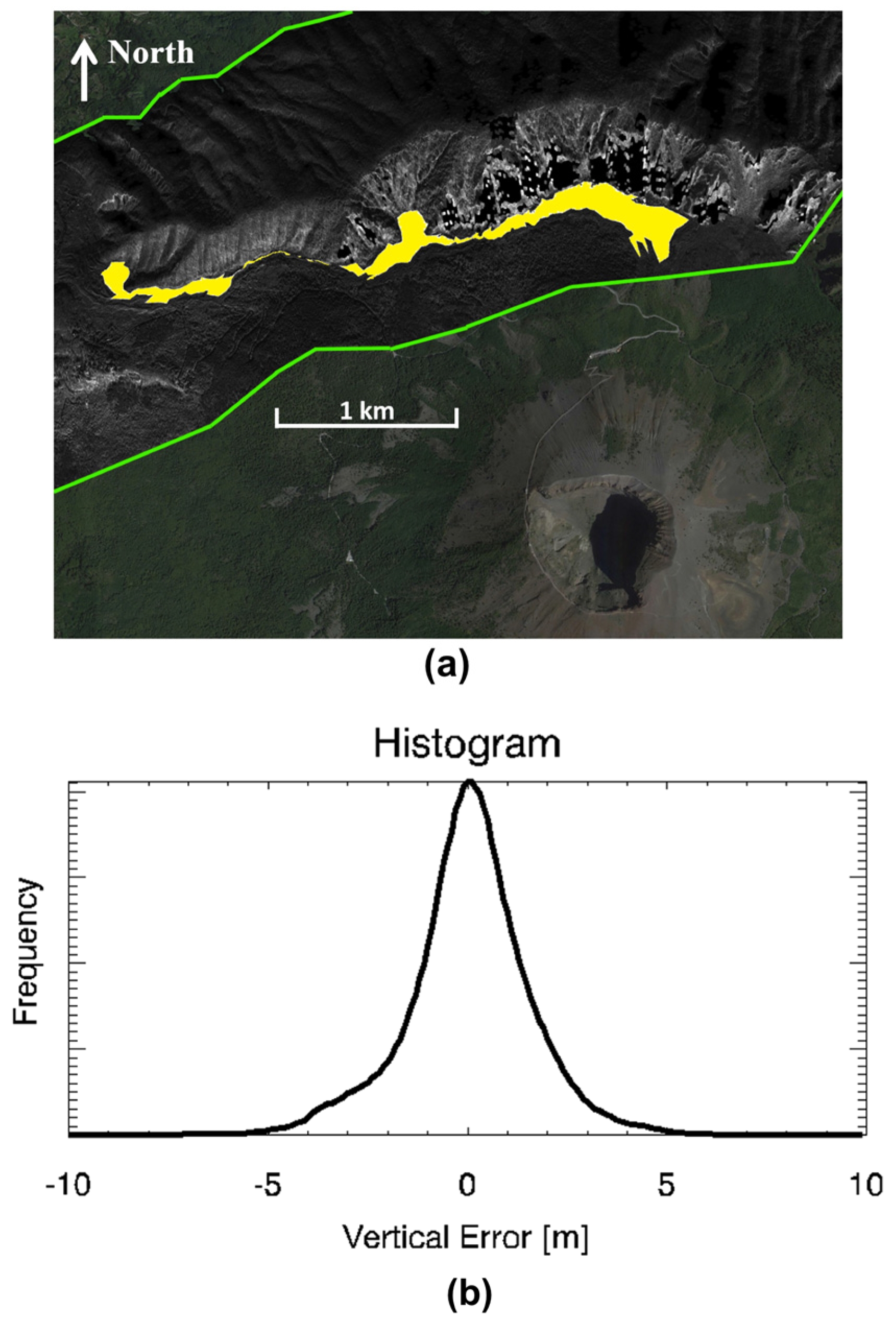
To further assess the vertical accuracy of the InSAeS4 system, we have also performed an extended scene analysis. To this aim, we have exploited a laser scanner DEM relevant to the 3 km long area covered by the 1944 lava flow on the Somma Vesuvio volcanic complex [
29]. In particular, such a DEM has been provided by the Osservatorio Vesuviano (OV) of the Istituto Nazionale di Geofisica e Vulcanologia (INGV). The test site is placed within the frames 1 and 2; however, for the 50 MHz acquisition (frame 1), it falls within a shadowing area. Accordingly, only comparison with the 400 MHz data (frame 2) has been possible: a zoom of the corresponding (geocoded) SLC is reported in
Figure 6a with highlighted the test site (yellow). Again, we have exploited only the interferogram with the largest baseline. By comparing our InSAeS4 DEM and the available laser scanner one we have obtained the histogram reported in
Figure 6b. In particular, we have measured a mean vertical error of 0.07 m with a standard deviation of 1.57 m. The latter result is thus worse than that obtained through the analysis carried out above by exploiting the CRs. To this regard, we note that the height of ambiguity relevant to the used baseline and the considered test area ranges from 75 m to 90 m. Accordingly, the standard deviation of the vertical error measured in the test area (1.57 m) turns out to be related to an interferometric phase error with standard deviation ranging approximately from 6° to 7°. Although this preliminary result is certainly fine, we are quite confident that it can be further improved, especially if we consider the vertical accuracy obtained in correspondence of the CRs. Indeed, the possible presence of the baseline tilt bias mentioned above, coupled with the azimuth-variant attitude instabilities of the airplane during the acquisition, could have been responsible for the presence of residual phase errors in the corresponding single-pass interferogram. These in turn may have affected the final interferometric DEM along both the azimuth and the range directions. Further investigation of these issues will be addressed in the future by planning new InSAeS4 flight missions aimed at providing comparisons with available reference laser scanner DEMs wider than that exploited in this work and possibly relevant to different test sites characterized by different topographic features.
Figure 6.
(
a) Zoom of the frame 2 of
Figure 3a. The lava flow erupted from the Somma Vesuvio volcanic complex in 1944 covered by the laser scanner DEM is highlighted in yellow; (
b) Histogram of the vertical difference between the InSAeS4 DEM and the laser scanner DEM in the yellow area of
Figure 6a.


 ,
, 
