Article

Cloud and Snow Discrimination for CCD Images of HJ-1A/B Constellation Based on Spectral Signature and Spatio-Temporal Context

1
Institute of Mountain Hazards and Environment, Chinese Academy of Sciences, Chengdu 610041, China
2
University of Chinese Academy of Sciences, Beijing 100049, China
3
Department of Geography, University of Maryland, College Park, MD 20742, USA
*
Author to whom correspondence should be addressed.
These authors contributed equally to this work.
Remote Sens. 2016, 8(1), 31; https://doi.org/10.3390/rs8010031
Submission received: 27 September 2015 / Revised: 14 December 2015 / Accepted: 25 December 2015 / Published: 5 January 2016

Abstract

:
It is highly desirable to accurately detect the clouds in satellite images before any kind of applications. However, clouds and snow discrimination in remote sensing images is a challenging task because of their similar spectral signature. The shortwave infrared (SWIR, e.g., Landsat TM 1.55–1.75 µm band) band is widely used for the separation of cloud and snow. However, for some sensors such as the CBERS-2 (China-Brazil Earth Resources Satellite), CBERS-4 and HJ-1A/B (HuanJing (HJ), which means environment in Chinese) that are designed without SWIR band, such methods are no longer practical. In this paper, a new practical method was proposed to discriminate clouds from snow through combining the spectral reflectance with the spatio-temporal contextual information. Taking the Mt. Gongga region, where there is frequent clouds and snow cover, in China as a case area, the detailed methodology was introduced on how to use the 181 scenes of HJ-1A/B CCD images in the year 2011 to discriminate clouds and snow in these images. Visual inspection revealed that clouds and snow pixels can be accurately separated by the proposed method. The pixel-level quantitative accuracy validation was conducted by comparing the detection results with the reference cloud masks generated by a random-tile validation scheme. The pixel-level validation results showed that the coefficient of determination (R2) between the reference cloud masks and the detection results was 0.95, and the average overall accuracy, precision and recall for clouds were 91.32%, 85.33% and 81.82%, respectively. The experimental results confirmed that the proposed method was effective at providing reasonable cloud mask for the SWIR-lacking HJ-1A/B CCD images. Since HJ-1A/B have been in orbit for over seven years and these satellites still run well, the proposed method is helpful for the cloud mask generation of the historical archive HJ-1A/B images and even similar sensors.

Graphical Abstract

1. Introduction

Accurate detection of clouds in satellite images is critically important for a wide range of applications [1]. It is the fundamental pre-processing step for the land cover classification [2], change detection [3], image compositing [4,5], or biophysical variables inversion [6,7]. Generally, undetected clouds in satellite images can introduce serious positive bias in aerosol concentration, increase land surface albedo and result in identification of land cover change where none occurred [8,9].
Precise detection of clouds in the images is a quite challenging work not only because of the complexity of clouds themselves but also the difficulty in clouds and snow discrimination [1]. Regarding the complexity of clouds, many types of clouds exist and different types of clouds have various spectral signature. The differences are mainly depended on cloud properties such as optical thickness, height, particle effective radius and thermodynamic phase [10,11]. In particular, thin cirrus clouds are notoriously difficult to be detected due to their mixture spectral signature with land surface [12,13]. Regarding the clouds and snow discrimination, the spectral signature of snow and clouds are both visually bright in the visible wavelengths. This spectral similarity makes them very difficult to be distinguished in visible bands. Moreover, the spectral reflectance of snow can also vary greatly with its properties like grain size, amount of impurities, and thickness of snowpack. Sometimes snow can have very similar spectral signature to certain clouds [9].
Over the years, a number of automated cloud detection methods have been developed based on the spectral signature (hereafter called spectral-based methods) [5,9,10,12,14,15,16,17]. Among different spectral bands, the shortwave infrared (SWIR, e.g., Landsat TM 1.55–1.75 µm band) band is most widely used for the clouds and snow discrimination. The primary reason is that the reflectance of snow is usually lower than clouds and therefore snow is generally darker than clouds in the SWIR wavelengths [18]. The Normalized Difference Snow Index (NDSI) [19,20], a combination of visible and SWIR, is very effective for snow and clouds separation [1,10,16]. For instance, it was used for the generation of the internal cloud and snow masking algorithm in the Landsat Ecosystem Disturbance Adaptive Processing System (LEDAPS) [21,22]. However, for some newly launched sensors without SWIR band, such as CBERS (China-Brazil Earth Resources Satellite), HJ-1A/B (HuanJing (HJ), which means environment in Chinese), the aforementioned spectral-based methods are no longer practical and the difficulty in discriminating cloud and snow for these sensors is even more serious.
Combining spectral signature with spatio-temporal context provides more complementary information for the clouds or snow detection process [1,8,23,24]. For temporal context, it has been used in the new algorithms development for a number of satellite sensors, including MODIS [8], Landsat [9], SPOT [25], and Sentinel-2 [23]. A direct and simple strategy using temporal context is to compare the spectral difference of cloudy images with a referenced clear image [23]. This kind of strategy based on the basic hypothesis that the presence of clouds will introduce high-frequency random changes, and by comparing with a clear-sky reference image, the cloud and snow can be easily separated (hereafter called temporal-based methods). However, there are also some limitations in the temporal-based methods. The main limitation comes from the revisit cycles of satellites, especially for the fine spatial resolution but long revisit cycle sensors like Landsat. Due to the long revisiting cycles for these satellites, the phenological variations of some land cover types in the revisit cycle, such as the deciduous forest, grassland, farmland, and the glacier may vary so greatly that the basic assumption that the change of reflectance was induced by cloud presentence might be invalid. Another limitation comes from the geometric location relationships between clouds and snow. If the clouds cover the same region of snow, the spectral differencing will weaken clouds spectral signature and consequently may cause omission errors. Moreover, SWIR band is usually still needed in most temporal-based algorithms [8,9,23], which limits their application for the sensors without SWIR bands.
For spatial contextual information, it can be defined as how the probability of presence of one object (or objects) is affected by its (or their) neighbors [26]. It is the relationship between the target object and synthesis information generated from the spatial environment [27,28]. Texture is the widely used spatial contextual information, and it refers to repeated local patterns and their regular arrangement of kinds of objects in the images [29]. The texture of clouds and snow are one of their important properties. Even though the texture element of clouds and snow is variable and unpredictable, they are still obviously different from the ground object texture features. On the basis of texture feature analysis, many scientists have done considerable works to improve the accuracy of cloud or snow detection [30,31,32,33]. However, most of the present texture-based algorithms assume that there is no snow in the cloudy images or no clouds in the snow covered images [33]. Besides, there are many types of texture features, and using more features does not naturally result in higher accuracy because of the Hughes effect [29]. Moreover, using more feature also result in a large computation cost [32].
The HJ-1A/B is a kind of new generation polar orbit constellation launched in September 2008 by China. It provides fine-resolution (30-m) images like Landsat, and dense observations (every two days revisiting), which is appropriate for capturing anthropogenic impacts and retrieving biophysical parameters over heterogeneous land surface [34]. However, for the lack of SWIR bands, the cloud detection method for HJ-1A/B CCD images is still under the exploration stage. It is noted that taking fully advantage of the spectral signature and spatio-temporal context information of HJ-1A/B might be a practical way to provide an accurate cloud mask. Taking HJ-1A/B CCD images as an example, this paper focused on the cloud and snow discrimination problem as follows: (1) paying special attention to the cloud and snow discrimination for HJ-1A/B CCD and HJ-1A/B CCD like SWIR band-lacking images; and (2) developing the practical cloud and snow discrimination method that can combine the spectral signature with spatio-temporal contextual information. The rest of this paper is organized as follows: Section 2 describes the study area, HJ-1A/B satellites, images pre-processing methods, and the data time series stack used in this paper. Section 3 presents the clouds and snow discrimination methodology. Section 4 shows the results and accuracy analysis. Section 5 discusses the advantages and limitations of the proposed methods. Section 6 presents the conclusions.

2. Study Area and Data
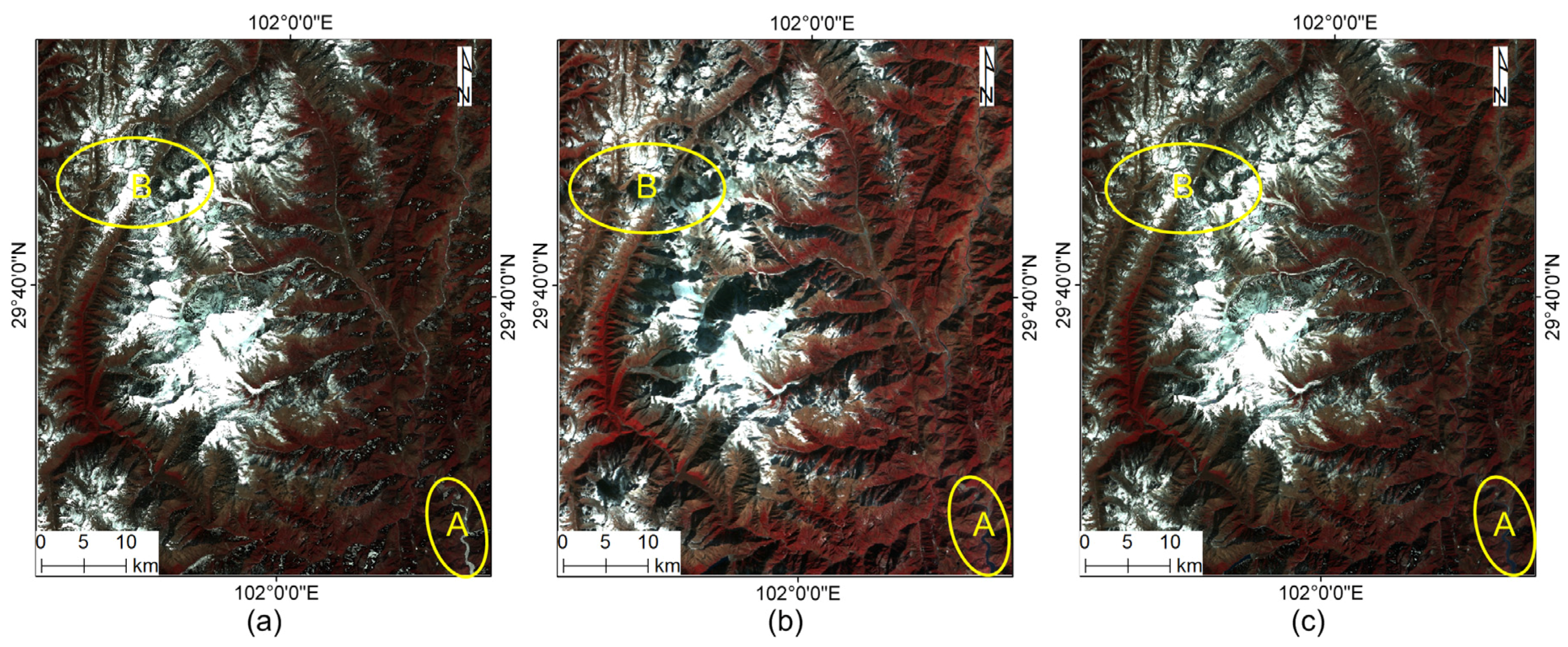
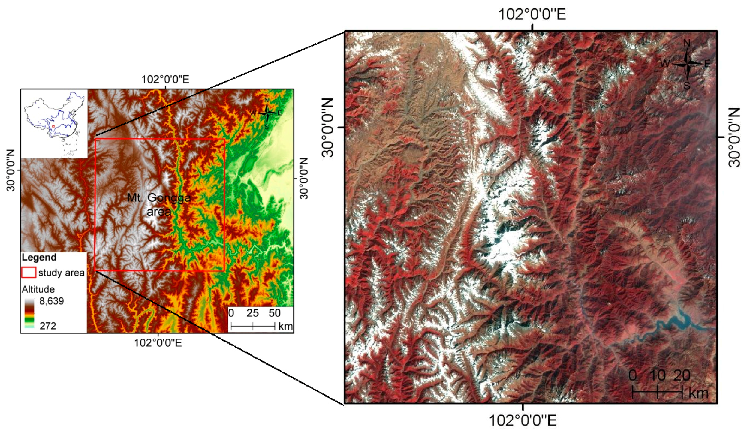
2.1. Study Area

In this study, Mt. Gongga region was chosen as the study area to evaluate the performance of the proposed method (Figure 1). This area was selected for the following reasons: (1) Mt. Gongga region is usually influenced by clouds and snow. This area is the highest peak in the eastern part of the Tibetan Plateau, and is one of the easternmost glacial areas in China [35]. It has persistent snow cover on the high mountains, especially in the upper snowline region where the altitude is about 4800 m. Besides, the annual precipitation of this region (3000 m, a.s.l) is about 1960 mm and most of the precipitation falls as rain from June to September, owing to the influence of Asian summer monsoons [36]. Because of the relatively concentrated precipitation during this period, the weather here is cloudy and the satellite images are usually contaminated by clouds. The frequent appearance of clouds and persistent snow make the area suitable for testing the algorithm’s discrimination ability; (2) The land cover of the study area is complex and the seasonal variations are obvious. The topography over this area is an alpine terrain with huge vertical relief (altitude ranging from 890 m to 7556 m). The influence of terrain on the formation of vertical vegetation zonation is evident, which further makes the phenological changes of vegetation vary greatly in a very short distance. This kind of phenological changes might introduce uncertainty into the temporal contextual analysis. An area about 22,500 km2 (150 km × 150 km) in the Mt. Gongga region was selected as the case region in this study.

2.2. HJ-1A/B Overview

The HJ-1A/B CCD images were chosen to develop and test the proposed method in this paper. Currently, the HJ-1 constellation consists of a pair of optical satellites (1A/B, launched in September 2008) and one microwave satellite (1C, launched in September 2013) [37]. The primary goal of the HJ-1A/B is to revisit any position in the world within two days for environmental monitoring and disaster mitigation. To achieve such a rapid global coverage, the two optical satellites, each of which has the four days revisit capability, are distributed in the same altitude and orbit plane, with a 180 degrees phase delay [38]. The HJ-1A/B are orbiting in a sun-synchronous circular orbit at 649.093 km altitude with a 10:30 a.m. ± 30 min descending node [39]. This satellite passing time is selected for the consideration of cloud cover and suitable sun illumination. It is also close to the Landsat local overpass time and matches Terra MODIS.
The payload of both HJ-1A/B includes two identical multi-spectral CCD image cameras that provide 30 meters spatial resolution and four bands observations from visible to near infrared: blue (Band 1, 0.43–0.52 μm), green (Band 2, 0.52–0.60 μm), red (Band 3, 0.63–0.69 μm) and near infrared (Band 4, 0.76–0.90 μm). The two CCD cameras are placed symmetrically with each other to the satellite nadir point. The placement makes the two CCD cameras equally divide the field of view and observe the earth side by side. The swath width of a single HJ1A/B CCD image is 360 km, while the combination of two CCD cameras obtains a swath width of 700 km. The CCD images can be freely obtained from the China Centre for Resource Satellite Data and Application (CRESDA). The relevant information is available at [40] with the interface in English.
Figure 1. The geolocation and the digital elevation model of the study area. The right image is the subset of 19 November 2011 HJ-1B CCD1 image shown with 4, 3, and 2 bands in red, green and blue, respectively.
Remotesensing 08 00031 g001

2.3. Image Pre-Processing

2.3.1. Geometric Correction

The HJ-1A/B images are distributed by the China Centre for Resource Satellite Data and Application (CRESDA), which are Level 2 products (after systematic geometric calibration). Precise registration of HJ CCD images was fulfilled by an automatic registration and topographic correction algorithm developed in [41]. The algorithm used the area-based image to image matching method to automatically select tie points between the geometrically corrected base images and HJ-1A/B CCD images. In this paper, the Global Land Survey (GLS) Landsat images from the year 2005 with geolocation error less than 30 m were used as base images [42]. The elevation data from the Shuttle Radar Topography Mission (SRTM) were used to correct the parallax errors caused by the local topographic relief [43].

2.3.2. Radiometric Calibration

The radiometric calibration is a fundamental process to eliminate the influence of the attenuation of the sensor photoelectric system [5]. It is especially important for images acquired from the constellation because of the significantly different attenuation of sensors in the different satellites [44]. The original digital number (DN) value recorded in HJ-1A/B multi-spectral CCD images were converted into Top Of Atmosphere (TOA) reflectance according to [45].

2.3.3. HJ-1A/B CCD Time Series Stack
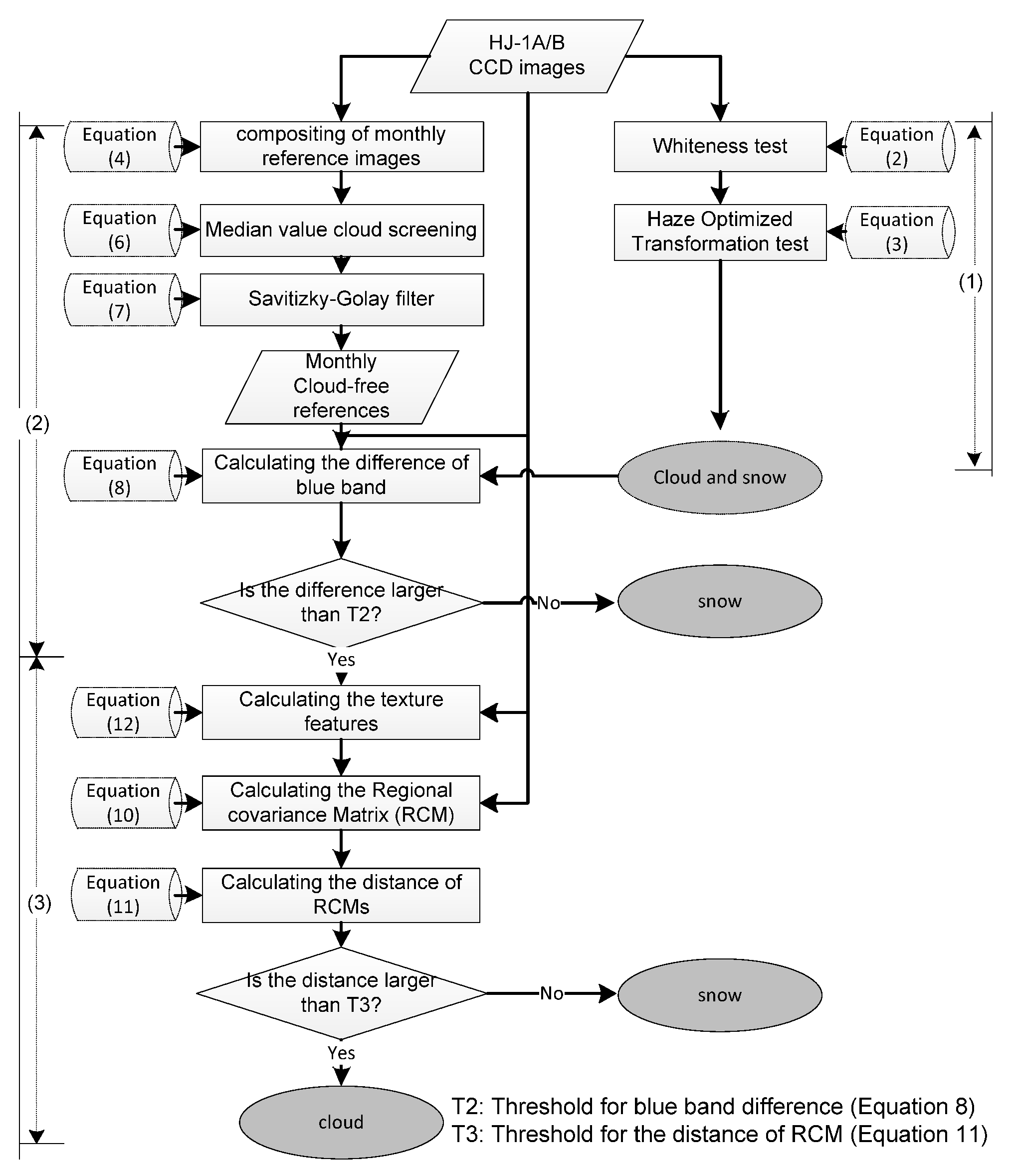
In this paper, the HJ-1A/B CCD time series stack (HJTSS) refers to a sequence of HJ-1A/B CCD images acquired at a nominal temporal interval for the particular geographical region. Same with the temporal resolution of HJ-1A/B CCD images, the temporal interval of HJTSS is approximately two days. To get the same geographical region of different HJ-1A/B CCD images, tiles with fixed dimension (number of rows and columns) instead of original path/row were used to organize the HJTSS. The orbit configuration of HJ-1A/B constellation was the main factor considered when using the fixed tiles [46]. Data volume of a single file was considered to determine the tile dimension. The tile was finally determined as 5000 × 5000 pixels to ensure manageable file sizes. In this paper, in total, 181 scenes of images from the year 2011 with the paths 14–19 and row 80 were selected as the test images.

3. Methodology

To overcome the shortcomings caused by the limited HJ-1A/B spectral bands, the new clouds and snow discrimination method that combines spectral information with spatio-temporal context is described in this section. The proposed method consists of three major stages, as shown in the flowchart (Figure 2): the initial spectral test, the temporal context test, and the spatial context test. In the first stage, clouds and snow pixels are extracted together based on the whiteness and the Haze Optimized Transformation (HOT) spectral tests. Then, in the second stage, the spectral differences between HJTSS image and the cloud-free reference image are calculated to discriminate most cloud from snow pixels. To get the cloud-free reference images, the HJTSS in each month are firstly composed based on a simple modified maximum NDVI value method in this stage. Considering there might be residual clouds in the composites, the median value cloud screening method is used to detect the residual clouds pixels, and then the Saviziky–Golay (S-G) filter-based reconstruction method is used to reconstruct the signatures of these clouds pixels. The above two stages are conducted on the spectral signatures and temporal domain. In the third stage, the synthetic spatial texture information calculated from the distance of Regional Covariance Matrix (RCM) is performed to correct the commission and omission errors in the first two stages. In the result, the clouds and snow pixels are finally discriminated.
Figure 2. Flowchart of the algorithm development.
Remotesensing 08 00031 g002

3.1. Initial Spectral Test for Cloud and Snow

Because of the similar spectral response of snow and cloud in the visible (VIS) and near-infrared (NIR) bands, two spectral tests were firstly used to extract both snow and cloud pixels for all of the HJTSS. The whiteness test (WT), originally proposed by Gomez-Chova et al. [47], was used as the fundamental test in this study. Since both thick cloud and snow are usually visually bright in the VIS and NIR band, the WT test is very effective for thick cloud and snow detection. It is based on following equations:
Mean V I S = ( band 1 + band 2 + band 3 )/ 3
W T = i = 1 3 |( band i mean V I S )/ Mean V I S | < 0.3
where bands 1–3 are the blue (0.43–0.52 μm), green (0.52–0.60 μm) and red (0.63–0.69 μm) band of HJ-1A/B CCD images, respectively.
The WT test enhanced the brightness difference between the visible bands and the overall brightness. It works well in the ENVIronmental SATellite (ENVISAT) and Medium Resolution Imaging Spectrometer (MERIS) [1]. However, it has some drawbacks on thin clouds detection because the brightness of thin clouds is directly related to the land cover and is variable. If the underlying surfaces of the thin cloud have a high reflectance, the cloudy pixels are bright. Otherwise, the brightness of the thin cloudy pixels may be close to that of the bright and cloudiness pixels [13]. To fix this problem, the HOT test developed by Zhang et al. [48] was used here to detect haze or thin clouds. The basic assumption of HOT is that the spectral response to diverse surface cover classes under clear-sky conditions is highly correlated in visible bands, but the spectral response to haze and thin clouds is highly sensitive to both blue and red wavelengths. Therefore, this correlation change can be used to detect haze and thin clouds [1,21]. It can be expressed as:
HOTtest = band 1 0.5 × band 3 0.08 > 0
where band 1 and 3 are the blue (0.43–0.52 μm) and red (0.63–0.69 μm) band of HJ-1A/B CCD images, respectively. It should be noted that due to the large reflectance of some bright pixels like barren rocks, turbid water or snow surface in the visible bands, the HOT might also include these pixels [1].

3.2. Separate Clouds from Snow Using the Temporal Context

As discussed earlier, because of the lack of SWIR band, separate clouds from snow using only visual to NIR spectral information is very difficult. However, from temporal aspect view, it is obvious that clouds cannot stay at the same place persistently due to its mobility characteristics. Therefore, it might be caused by the presence of clouds if surface reflectance has a big variation in time series observation [23]. The temporal context is the effective information and could be used to separate clouds from snow.

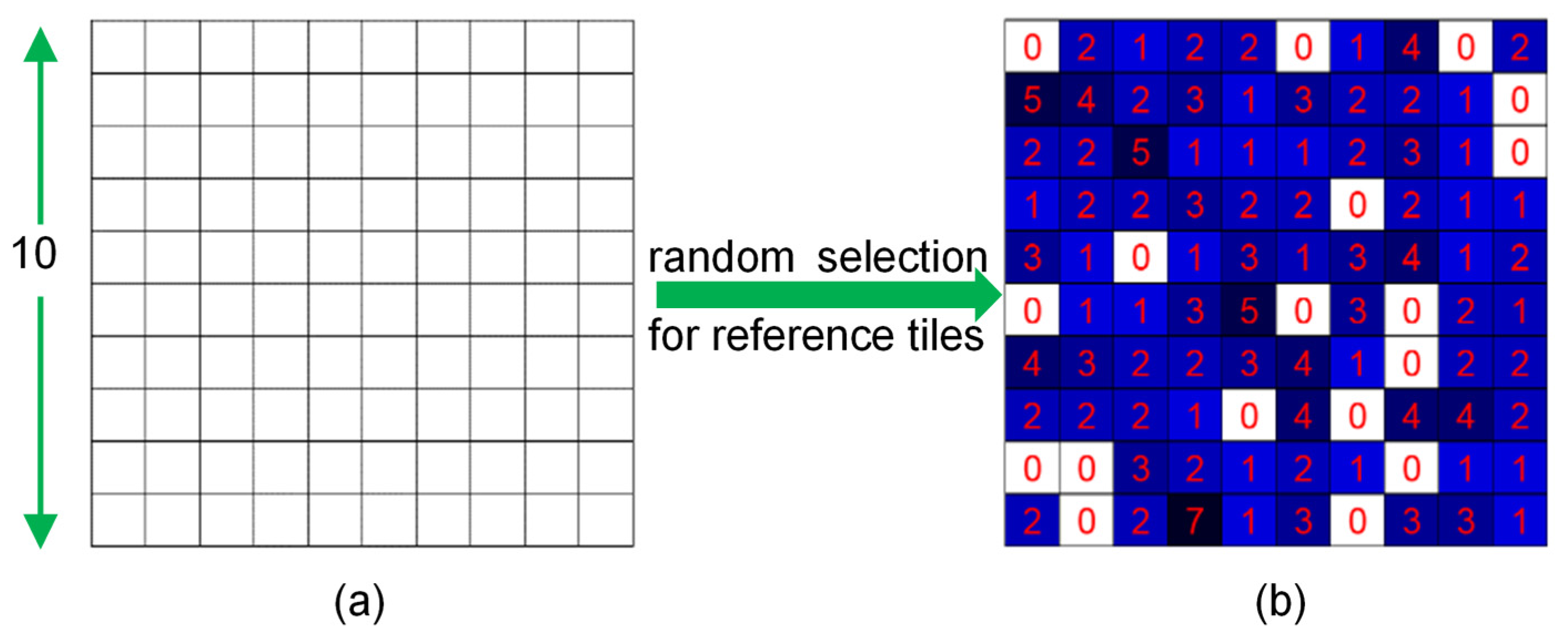
3.2.1. Compositing for the Monthly Cloud-Free Reference Images

A cloud-free reference image was firstly needed to detect the spectral variation of clouds in the HJTSS. Considering the cloud-free images are usually difficult to be acquired, reference images in this paper were composited from the partly cloudy images in each month. Many image compositing methods have been reported in the literature, which usually applied the minimum or maximum criteria [49,50,51,52,53]. Among these methods, the maximum NDVI value method is widely used because it can obtain the optimum vegetation observation and eliminate the cloud shadow to some extent. However, recent studies also noted that the compositing results from the maximum NDVI value method (Figure 3a) fails on the water surface because of the higher NDVI for cloud than water (As shown in area A) [53]. On the other hand, the composites produced from minimum blue band (Figure 3b) can chose the “clearest” pixel in a certain time window [52]. It performed better than the maximum NDVI over open water area, but it was still apparently affected by the contamination of cloud shadows (area B) because of the lower reflectance of cloud shadow than that of clear land. To take advantage of the maximum NDVI method on selecting vegetation pixels and the minimum blue method on choosing clear pixels, a simple combined criterion (Equation (4)) was used here for compositing of the references images.
{ max ( N D V I t )      WaterTest = 0 min ( ρ t blue )           WaterTest = 1
where
Water Test = ( N D V I < 0.01  and Band  4 < 0.11 ) or ( N D V I < 0.1  and Band  4 < 0.05 )
This combined criterion kept the open water information when clouds presented over the same geographic region with open water. It also preserved the optimal vegetation pixels in the compositing procedure. The water pixels were identified in the combined criterion firstly based on its physical characteristics: the lower signal observed in NIR wavelengths than visible wavelengths. The threshold of NDVI and Band 4 was inherited from the LEDAPS internal cloud masking algorithm where the number 0 represents none water pixel and 1 represents water pixel [21]. Figure 3c illustrated the image generated from the combined compositing criterion. Obviously, the composited results performed better than the above two methods and the quality of the composites was substantially improved.
Figure 3. Cloud-free images generated by different composting methods: (a) Maximum NDVI; (b) Minimum blue; and (c) Combined compositing criterion.
Remotesensing 08 00031 g003

3.2.2. Post-Processing for the Composites

Since some residual clouds may still exist in the above composites, the composites need to be further processed to get the cloud-free reference images. A median value cloud screening method was applied firstly to detect those residual clouds. This method is based on the assumption that the position of clouds will changed rapidly and clouds cannot stay at the same place persistently, and therefore the reflectance of clouds pixels will always be higher than the median values of the entire time series at the same location [9,54]. Because the short wavelengths are more sensitive to clouds, the blue band TOA reflectance was used in the median value cloud screening method. If the blue band TOA reflectance of a pixel in the composites is equal to or higher than the median value plus a constant, it is identified as a residual cloud pixel (Equation (6)).
ρ ( band  1 , x j ) median ( ρ ( band  1 , x { 1 , 2 , 3 , 12 } ) ) + T 1
where, ρ ( band 1 , x j ) is the observed blue band TOA reflectance at month x for the jth pixel. T1 is a constant to ensure that if the entire time series of a pixel is cloud free, pixels with blue band TOA reflectance higher than the median value will not be misidentified as clouds. Based on a test of all 181 images, the constant T1 was determined as 0.04.
After successfully identified by the median value cloud screening method, the residual clouds pixels were then reconstructed by the S-G filter-based reconstruction method [55]. In the reconstruction method, the linear interpolation was firstly used to roughly predict the TOA reflectance of cloud pixels using the none-cloud TOA values from adjacent dates. Then, the S-G filter-based reconstruction method was used to estimate the TOA reflectance of those cloud pixels. The S-G filter is a simplified least-squares-fit convolution for smoothing and computing derivate of a set of consecutive values [56]. It uses a high-order polynomial instead of a constant to achieve the least-squares fitting within the sliding window to approximate the base function. Taking a fixed number of points in the vicinity point to fit a polynomial, it gives the smooth value of the vicinity point according to the polynomial during the fitting progress [57].
ρ ^ ( b , x j ) = i = m i = m C i ρ j + i N
where ρ ^ ( b , x j ) is the predicted TOA reflectance of the bth band at month j for the x cloud pixel, Ci is the coefficient given by the Savizky–Golay filter and N is the number of pixels in the smoothing window, which is equal to the smoothing window size (2m + 1).
To illustrate the reconstruction effects for those residual clouds, Figure 4 shows the comparison before and after reconstruction of three typical areas. Obviously, the median method successfully captured the residual clouds in the composites, and after reconstruction, those cloudy areas transited smoothly with those clear grounds.
Figure 4. Comparison of residual clouds in the monthly composited images and their Savizky–Golay filter reconstruction results of May, June and November: (a) the residual clouds in the monthly composites; and (b) the residual clouds mask generated by the median value method, where the yellow color is clouds and green color is background. The identified clouds are a little larger in extent because of three pixel dilation of clouds to exclude some thin edges of clouds; (c) The reconstruction results by the Savizky–Golay filter.
Remotesensing 08 00031 g004

3.2.3. Cloud and Snow Discrimination by the Reference Images

Based on Hagolle et al. [23], a pixel can be flagged as a cloud pixel if its blue band TOA reflectance satisfies the following multi-temporal criterion:
[ ρ blue ( D ) ρ blue ( D r )] > T 2 × ( 1 + ( D D r )/ D T , n )
where ρ blue ( D ) is the blue band TOA reflectance of a given pixel at date D, and ρ blue ( D r ) is the corresponding blue band TOA reflectance of cloud-free reference images, which is the monthly composited reference images in this paper. D D r is the number of days from the test date to reference date and expressed in days. It was calculated from the acquired date of a given image and the Day Of Year (DOY) data layer stored in the composited images. The blue band difference was used instead of other bands because of the relatively high reflectance for clouds and snow and low reflectance for most of the earth surface in this band [9].
When dates between the reference and cloud images are very close, the threshold T2 for Equation (8) was set as 0.03 according to the reflectance difference analysis in [23], and the DT,n was set as a constant which was 30 days. However, due to the different set of spectral width, the optimal threshold for HJ CCD images needs to be adjusted. To find the optimal threshold for HJ CCD images, we analyzed the change of TOA reflectance for snow, cloud and clear land pixels at the two-day interval for all the HJ CCD images in 2011. In Figure 5, it is noted that a threshold of 0.05 can be better used to separate cloud from clear land. The DT,n was set according to the length of days in each month.
Figure 5. Histogram for Top Of Atmosphere (TOA) reflectance difference for the snow, clouds and clear ground pixels at two-day intervals.
Remotesensing 08 00031 g005
Although the multi-temporal criterion is efficient to separate most of cloud from snow pixels, it still has some drawbacks. For example, some thin clouds might be regarded as clear ground since the spectral variation in multi-temporal images is quite slow. Besides, snow pixels with brighter reflectance than reference images may be mis-detected as clouds according to Equation (8). Therefore, the following spatial context criterion was used to further process the incorrectly detected and undetected clouds.

3.3. Separate Clouds from Snow Using the Synthesize Spatial Context

3.3.1. Theoretical Basis

To cope with the above problems, the spatial context of clouds and snow were further used in the third stage of the proposed method. The RCM that is widely used in the target detection and tracking [58,59] field was conducted to synthesize the multiple texture features in this stage. RCM is a fast region descriptor for object detection and classification [60]. Different from only using one texture feature, the RCM can synthesize several image statistics, including the spectral reflectance, gradient or filter responses as image features and then use the covariance of these features as the region descriptor. It is shown that large rotations and illumination changes can be absorbed by the RCM, and the noise corrupting individual samples can also be filtered out [61]. The similarity measurement of two RCM is the distance metric, which is defined on the positive definite symmetric matrices because the covariance matrices are not elements of the Euclidean space.
For the computing of the RCM, let I be the remote sensing images, and F be the W × H × d dimensional features extracted from I:
F(x,y) = φ(I,x,y)
where the function φ can be any mapping such as the gray values, color, gradients and filter response. x and y are the row and column in the image coordinate system. For a given rectangular R F , let { z k } k = 1 , , n be the d-dimensional feature points inside R. The regional R can be represented with the d × d covariance matrix of the feature points:
C R = 1 n 1 k = 1 n ( z k μ ) ( z k μ ) T
where μ is the mean of the points, n is the number of pixels.
Since the distance between RCM does not lie in Euclidean space, the similarity of two covariance matrices can be measured by Förstner et al. [62]:
d ( C 0 , C T ) = i = 1 n ln 2 ( λ i ( C 0 , C T ) )
where d ( C 0 , C T ) is the distance for RCM between reference C0 and the detecting images CT. { λ i ( C 0 , C T ) } i = 1 n is the generalized eigenvalues of C0 and CT.

3.3.2. RCM Implement for Cloud and Snow Discrimination

For cloud and snow discrimination, given a test and reference image, the aim of using RCM is to enhance the information of the cloudy area and weaken that of cloudless area. Since the presence of clouds makes both spectral signature and texture characters of cloud region change dramatically compared with reference images, the distance of RCM is sensitive to the cloudy area and insensitive to those clear grounds. When RCM of HJTSS and reference images shows a larger distance than the threshold, it may be caused by the clouds contamination.
Four bands TOA reflectance and the calculated NDVI were used for the development of RCM for both HJTSS and monthly reference composites. The responses from the Sobel operator and Laplace of Gaussian (LoG) operator, representing the first and second order derivatives, were also conducted as texture features and were included in RCM. Sobel operator is a non-linear edge enhancement detector filter that uses an approximation of the Sobel function to get the first order derivatives of a given image. It has a simple form and is widely used in the edge detection field. The LoG operator firstly uses the Gaussian convolution filter to reduce the image noise, and then adopts the Laplace operator to seek the zero crossing point of the second derivative of the image for edge detection, which improves the robustness to the noise and discrete points. The homogeneity feature, which is extracted from Gray Level Co-occurrence Matrix (GLCM) and measures the closeness of the distribution of elements in the GLCM to the GLCM diagonal [63], was also introduced into RCM. The eight-dimensional feature vector can be written in Equation (12) as defined in Equation (9):
F ( x , y ) = [ b 1 4 ( x , y ) , N D V I ( x , y ) , S o b e l ( x , y ) , L o G ( x , y ) , H o m o _ G L C M ] T
where, b1–4(x, y) are the four bands TOA reflectance of HJ-1A/B images; NDVI(x, y) is calculated from band 4 and 3; Sobel(x, y) is the blue band response from Sobel operator; LoG(x, y) is the blue band response from Laplace of Gaussian operator; and Homo_GLCM is the homogeneity feature extracted from GLCM, (x, y) are the pixel locations.
The implementation steps were as follows. Firstly, a small region with 3 × 3 pixel matrix was placed inside the image, as showed in Figure 6. The RCMs of the small region were first calculated for the test (C1) and reference image (C2) through Equation (10). Then the distance between C1 and C2 was calculated according to Equation (11). A threshold of 6.50 was chosen for the optimal cloud and snow discrimination (Figure 6). This threshold was derived based on a test of all the 181 images. For most of clear and snow pixels, the distance between references and the HJTSS were always less than 6.50. While if there were clouds, even some thin clouds presented, the distance between RCMs increased dramatically and was usually larger than 6.50. Therefore, this threshold of 6.50 was helpful to discriminate the un-detected thin cloud and mis-detected snow pixels in the first two steps. After the RCM analysis, all cloudy pixels were dilated by three pixels in all eight connected directions to remove the surrounding pixels that may be partially influenced by clouds.
Figure 6. Image features construction and Regional Covariance Matrix (RCM) differences detection.
Remotesensing 08 00031 g006

3.4. Accuracy Assessment

The following three different accuracies measures, which were the overall accuracy, precision and recall, were used to assess the accuracy of the algorithm results. Take the cloud as an example. Define the True Positives (TP) as the number of clouds correctly labeled as belonging to clouds in the algorithm, False Positives (FP) as the number of none-clouds incorrectly labeled as belonging to clouds, False Negatives (FN) as number of clouds incorrectly labeled as belonging to none-clouds, and True Negatives (TN) as number of none clouds which also labeled as belonging to none clouds. The accuracy, precision and recall are then defined as [64]:
Overall Accuracy = (TP + TN)/(TP + TN + FP + FN)
Precision = TP/(TP + FP)
Recall = TP/(TP + FN)
In the clouds case, precision denotes the proportion of truly cloud pixels in the cloud detection results, while recall is of all pixels that are actually clouds in the image, what fraction of them were detected as clouds. For precision and recall, they are better reflects the errors of omission and commission for the snow and cloud classes than overall accuracy. These three accuracies for cloud and snow were calculated separately.

4. Results and Analysis
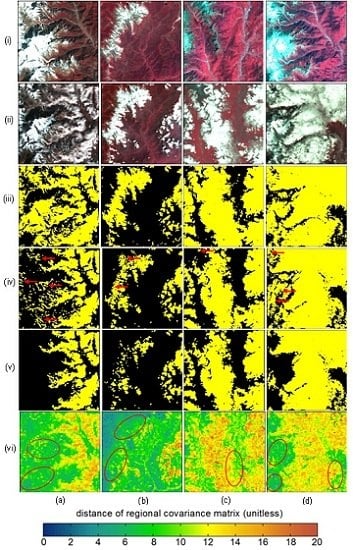
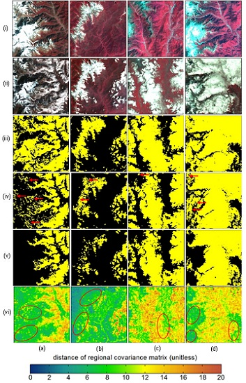
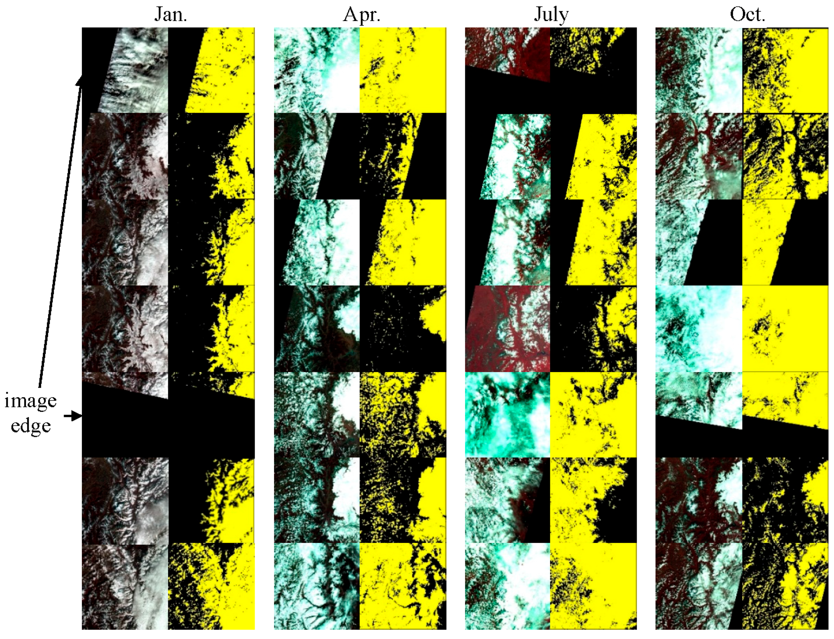
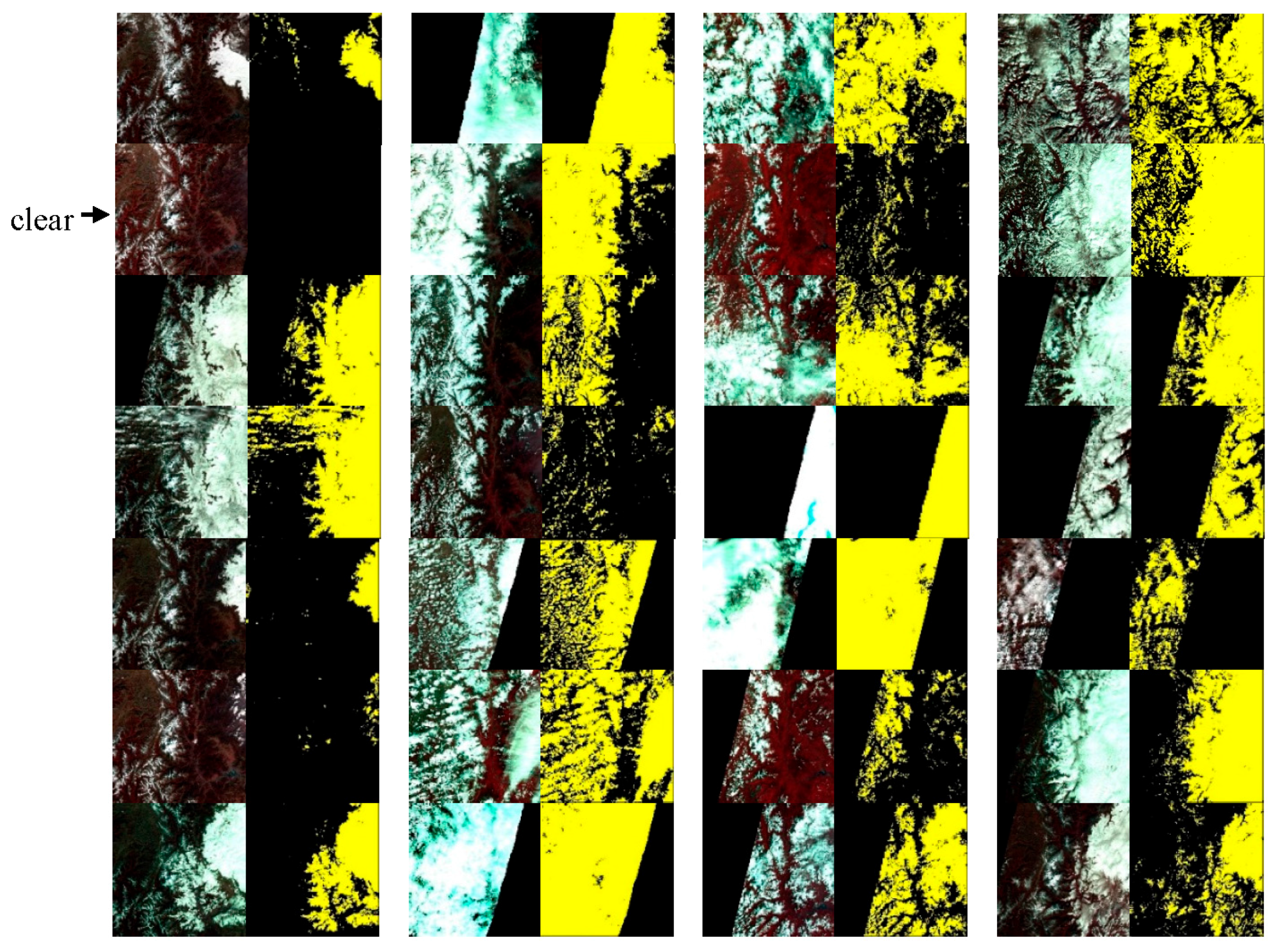
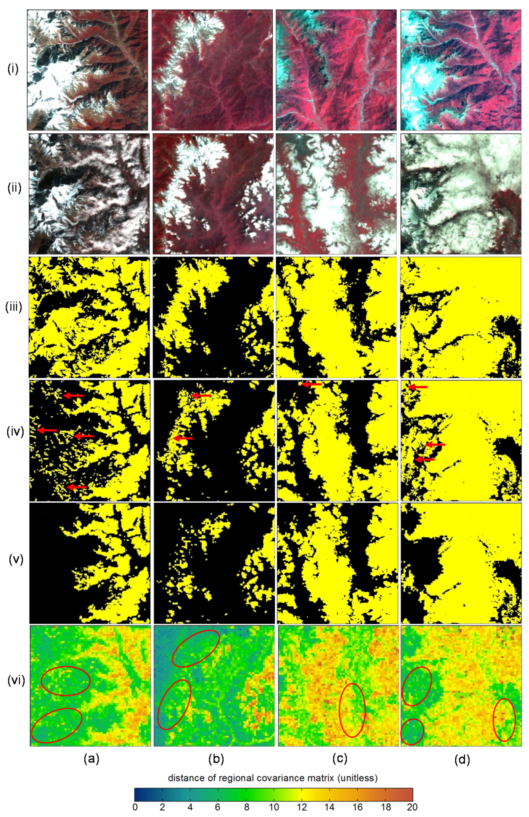
4.1. Mask Results

Figure 7 depicts the cloud and snow detection results for HJ-1A/B images from four different dates. By visually comparing the results with the false color composites (RGB = 4, 3, 2), it is clear that the algorithm developed in this study can accurately separate the cloud and snow pixels. Figure 7a was a winter image acquired at 14 January 2011 with obvious clouds and snow over the whole image. The mask results showed its strong ability in excluding the snow pixels from cloud pixels. On the other hand, Figure 7b was a spring image acquired at 14 April 2011 with large variability in surface reflectance. The red quadrangles in the Figure 7b were covered by bare rocks (see red arrows) and snow (see yellow arrows), which were the bright earth surfaces in the current color scheme. The mask results worked well in terms of identifying clouds in areas with very bright land surface. Figure 7c was an image acquired at 12 June 2011, with many thick and thin cirrus clouds (see the yellow arrows). It is noted that the thin clouds were also accurately identified through the proposed method. Figure 7d was acquired at 1 September 2011 with bare rocks (see yellow arrow) and thick aerosols in the image (see the red arrow). In the mask result, the aerosols and bare bright rocks were successfully excluded and the cloudy pixels were also accurately identified.
Figure 7. Cloud and snow separation results for four different dates. (a) Result of HJ1A-CCD1-20110114 scene; (b) Result of HJ1A-CCD1-20110414 scene; (c) Result of 12 June HJ1A-CCD2-20110612 scene; and (d) Result of HJ1B-CCD1-20110901 scene. For each date, (Upper left) and (Upper right) show false color composited HJ images and the corresponding cloud mask; and (Lower left) and (Low right) images are enlargements of (Upper left) and (Upper right) images, respectively with a size of 1000 pixels × 1000 pixels.
Remotesensing 08 00031 g007
Figure 8 provides an illustration of the algorithm performance for the four middle month of every season of the year. The standard seasonal definition for the Northern Hemisphere adopted by the climate modeling community is used where spring is defined by the months March to May. Each column contained 14 images. Time intervals for most of these images were two days because of the two days revisiting period for the HJ-1A/B constellation. The mobility of clouds and the temporal contextual information provided by different periods over the same geographical regions, clearly visible in these images, was critical to the success of the developed algorithm. Generally, the algorithm developed in this paper worked well for most of the images for every season. The performance of the algorithm was robust regardless of the snow brightness. In general, it achieved the best performance when the surface condition was stable, for example in July and October with durable snow cover. However, the algorithm tended to overestimate cloudiness during sudden snow fall or snowmelt period when surface changes were rapid and the composites reference had less snow than these days. For instance, the first column, which represented the winter season, showed overestimating of some clouds. The qualitative evaluation was an important aspect of the development of the algorithm. To more rigorously assess its accuracy, reference data were used.
Figure 8. Examples of performance of the proposed algorithm for 150 km × 150 km Mt. Gongga area for the middle month of each season of the year 2011. The standard seasonal definition for the Northern Hemisphere adopted by the climate modeling community is used, where spring is defined by the months March to May. False color composited images with bands 4, 3, and 2 in red, green and blue, respectively, are shown on the left, and cloud masks are shown on the right with yellow color.
Remotesensing 08 00031 g008aRemotesensing 08 00031 g008b

4.2. Performance of Each Stage for the Cloud and Snow Discrimination

To illustrate the effectiveness of each stage for cloud and snow discrimination in the proposed method, Figure 9 shows the HJ-1A/B images acquired in four different dates, the corresponding monthly reference composites, initial mask results from spectral test, mask results after temporal contextual test, final mask results after spatial contextual test, and the distance of RCM between references images and HJ-1A/B images, respectively.
In general, the improvement for the cloud and snow discrimination for each stage can be evidently elucidated from Figure 9. For the initial spectral test (Figure 9, row iii), it is apparent that the snow and clouds were accurately separated from clear grounds. However, snow and clouds pixels can only be extracted together in this stage due to their spectral similarity. On the other hand, after the temporal contextual test, many snow pixels were dramatically eliminated from clouds. According to statistics for the four case areas in Figure 9, approximately 79.98% misclassified clouds pixels from initial spectral test were successfully separated by temporal contextual test. However, it is also noted that some snow pixels still existed in the temporal test results (see red arrow). Particularly, after using of RCM the snow pixels are efficiently excluded from clouds (in the red ellipse). The RCM test further eliminated 20.02% of the misclassified cloud pixels from the temporal contextual test.
Figure 9. The comparison before and after using the regional covariance matrix (RCM). Column (ad) are the HJ images acquired in 6 January, 30 April, 29 June and 10 October and its corresponding cloud and snow discriminating results in each stage, respectively. The first and second row are the corresponding monthly composited images and the original images shown in false color with bands 4, 3, and 2 in red, green and blue, respectively. The third, fourth and fifth rows are the cloud masks for spectral test, temporal test, and texture test, respectively. The sixth row is the distance of RCM with its color bar under the bottom of this figure.
Remotesensing 08 00031 g009

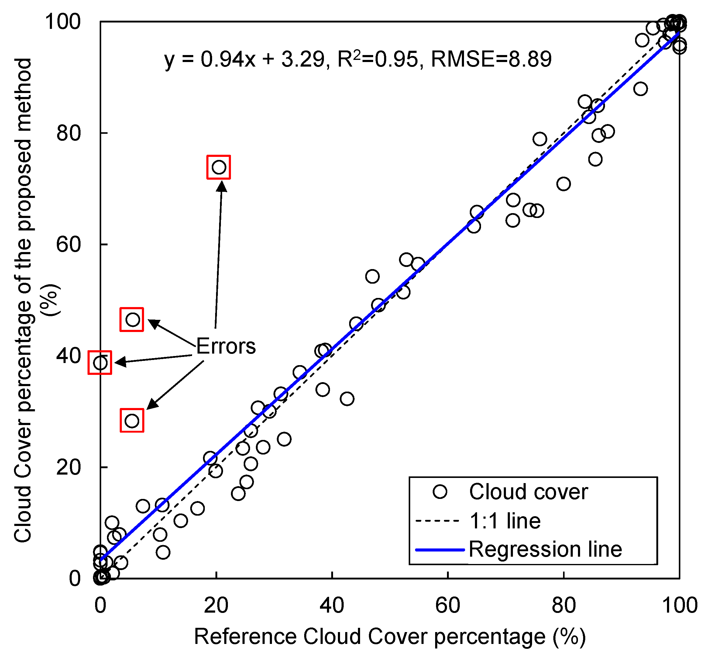
4.3. Pixel Accuracy Assessment

Based on the visual assessment, clouds and snow pixels in HJTSS from different dates can be effectively discriminated. To further quantitatively assess the accuracy of the results, a reference cloud mask for each image was derived and the pixel-level accuracy was evaluated. The reference cloud masks were derived by a supervised classification method and manual editing method as follows. First, the object-based classification algorithm was used to segment the images into objects. Then, sample objects of both clouds and snow were chosen as the training datasets to construct a decision tree to classify the segmented objects into clouds, snow and clear grounds. Last, the classification results were edited manually to eliminate misclassification errors, leading to the production of the final reference masks.
To reduce the manual editing effort, a pseudo-random number function was used to randomly select a tile with 500 pixels × 500 pixels dimension within each image as the reference cloud mask. The HJTSS were firstly divided into 10 × 10 tiles, which were numbered consecutively from 1 to 100 from left to right and top to bottom (Figure 10a). Then, a random positive number, representing the selected tile, was selected from 1 to 100 using the psedo-random number function. The final selected reference tiles for all the HJTSS are shown in Figure 10b. Each number in the grid represents how many times this tile was chose.
Figure 10. (a) is the tiles grid for the reference masks and (b) is the selection results for each tile.
Remotesensing 08 00031 g010
Figure 11 displays the scatter plots of cloud cover percentage between all the reference cloud masks and the algorithm cloud masks. Overall, estimates of percent cloud cover from our proposed method were very accurate (Figure 11), with an R2 of more than 0.9. The slope of the regression line was 0.94, with a very small interception (3.29%), and relatively small Root Mean Square Error (RMSE) (8.89%). However, from the above comparison of all the reference masks, it is also noted that the agreement for some of the days were relatively lower than other days. These disagreements were mainly caused by the sudden snowfall event after examination, which will be further discussed in Section 5.3.
Figure 12 illustrates the histograms of the overall accuracy, precision and recall for clouds and snow, respectively. At the pixel scale, for clouds, the average overall accuracy was 91.32% with a small standard deviation of 6.5% (Figure 12a). The average precision was 85.33% (Figure 12b) with a standard deviation of 14.17%. Moreover, the average recall was 81.82% (Figure 12c) with a standard deviation of 12.31%. For snow, the average overall accuracy was 92.80% with a small standard deviation of 5.3% (Figure 12d). The average precision was 82.18% (Figure 12e) with a standard deviation of 15.28%. Moreover, the average recall was 82.81% (Figure 12f) with a standard deviation of 14.78%. It is noted that the overall accuracy and precision of clouds were slightly lower than that of snow. The reasons were mainly attributed to the three pixels dilated (in all eight connected directions) for all cloud pixels. The lower precision of clouds was reasonable because un-detected clouds will more greatly influence future image applications than a little lost data by buffered cloud edges. Because the spectral variation of clouds was larger than snow pixels, especially for those thin clouds, clouds will be more easily detected as clear ground. Therefore, the recall of clouds was slightly lower than that of snow.
Figure 11. Visual cloud cover vs. detected cloud cover for the all the reference masks in the year 2011.
Remotesensing 08 00031 g011
Figure 12. Histogram of the cloud overall accuracy, precision and recall: (ac) accuracy, precision and recall for clouds, respectively; and (df) for snow.
Remotesensing 08 00031 g012

5. Discussions

5.1. The Effectiveness of the Temporal Contextual Information for Cloud and Snow Discrimination

Temporal characteristics of satellite images offer important textural information for the discrimination of clouds and snow. With the added temporal information, only three optical and one NIR band were used in the proposed approach, making up for the SWIR band-lacking shortcomings for HJ-1A/B CCD images. The temporal information can be used in the following two ways for the separation of cloud and snow: (1) using the multi-temporal images to compose a cloud-free reference image and then make the spectral difference analysis [23,65]; and (2) making the time series analysis for all the multi-temporal images and then detect the sudden changes caused by clouds [8,9,24]. In this paper, the above two methods were applied to generate the monthly time series of cloud-free reference images. Those reference images were successfully used for clouds and snow discrimination.
For the compositing of the cloud-free reference images, the setting of time interval is an important factor that will influence final detection accuracy [13]. If the time interval is too short, the available images in the time window will be very limited, and the composites might still have many residual clouds. Two kinds of cloud underestimation condition will be caused when the reference images still have clouds. One is that snow in the HJTSS appears at the same location of clouds. At this condition, the difference between HJTSS and reference images would be the difference between snow and clouds (close to 0) and therefore omission errors will be introduced. The other underestimation condition is that clouds in the HJTSS appear in the same clouds region. This condition will also cause omission errors because the composites still have residual clouds. On the contrary, if the time interval is too long such as the seasonal compositing, although increased observation frequency could further eliminate the clouds influence for composites, the regular phenological changes of geographical features might be another important uncertainty source. The following two aspects were taken into consideration when the time interval was set as monthly composites in this paper. Firstly, for the revisiting period of HJ-1A/B is two days, there will be enough images to composite a nearly clear-sky reference image in one month [46]. According to the spectral changes analysis and the temporal filter, the totally cloud-free references images can be acquired for every month. Secondly, considering the spectral variation for most of vegetation and land surface are slightly in a month, monthly composites is representative and suitable for the cloud detection. Despite this, a clear-sky sub-monthly composite reference image such as the semi-month would be better than the monthly composites due to the shorter temporal difference between the test and reference images.

5.2. The Usefulness of Spatial Contextual Information for Cloud and Snow Discrimination

Texture refers to the repeated local patterns and their regular arrangement of the ground objects in the images. The texture features can better reflect the macroscopic properties and the detail structures of the ground objects than a single pixel. Correctly understanding the texture difference of clouds and snow can provide the important basis for their discrimination. To our knowledge, the texture of clouds is a type of random texture. Even though the texture element of clouds is variable and unpredictable, it is greatly different from the texture feature of ground object and snow area. For instance, the edge of the cloud contains gray level jump characteristics, and the part of the cloud is similarity to the whole. The cloud cluster has a certain fractals similarity [30]. On the other hand, the texture of snow in remote sensing images usually is bumpy because the influence from terrain relief, vegetation or man-made features. The gray gradient of snow usually is larger than that of clouds.
The frequently-used texture features of cloud are the average gradient, fractal dimension and GLCM [63]. In this paper, texture features derives from gray gradient (the first and second order derivatives) and the spatial correlation properties of gray (that is the GLCM) were used for clouds and snow discrimination. These texture features has been demonstrated effectively for cloud or snow detection. However, some other texture features such as GLCM [63], pixel shape index [66], morphological profiles [67], and wavelet-based texture [68] can also evidently improve the accuracy of snow or cloud cover extraction. However, increasing the number of texture features does not consequently lead to higher accuracy but will result in a large computing cost [29,32]. Therefore, more efforts in the future can be put into find the representative and less computing-consuming features to improve the efficiency and accuracy.
The RCM was used to synthesize all the spectral and texture features into a distance index between HJTSS and reference images to express their similarity at the regional scales. The RCM enhanced the cloud and snow region difference at the regional scale, which is helpful for the discriminating snow from clouds for the following two cases. The first case is that snow areas in HJTSS are larger than that in reference images. In this condition, since the reference images were composited from the HJTSS in each month, the smaller snow areas in reference image than HJTSS will cause the overestimate of clouds and consequently underestimate snow pixels. Another case is that the snow spectral signature in HJTSS varied higher than the cloud spectral threshold (T1 in Equation (6)). In this condition, due to the melt effects of snow or differences in observation conditions, the reflectance difference between snow in HJTSS and reference image might also introduce overestimate of clouds. Fortunately, since the RCM was calculated from a series of regional texture information, it has a strong capability of filtering out the noise corrupting individual samples. Therefore, both of the above cases can be eliminated at the regional scales by RCM.

5.3. Error Sources of the Proposed Method

Overall, the cloud and snow detection results indicated that the proposed method can achieve a good performance for the discrimination of cloud and snow in HJ-1A/B images with only four bands within a whole year. However, several error sources which might influence the algorithm accuracy should also be pointed out. The first error source came from the way which the cloud boundary was treated. In order to remove the cloud surrounding pixels that may be partially contaminated, the proposed method dilated all cloud pixels by three pixels in all eight connected directions, which might overestimate clouds areas. Therefore, the overall accuracy and precision of clouds were slightly lower than that of snow (As shown in Figure 12). Another error source might be the undetected cirrus clouds. To our knowledge, the detection of cirrus clouds is very challenging since regions covered by cirrus clouds not only contain signature and texture information from clouds but also from the ground features [13,69]. For example, Kovalskyy and Roy [12] recently found that about 7% cirrus contaminated pixels in historical conterminous United States Landsat archive were undetected. These thin and cirrus clouds might also be omitted because of the lack of cirrus cloud sensitive bands (e.g., Landsat-8 cirrus band). Finally, while sudden snowfall happens (As shown in Figure 11), some snow pixels might be incorrectly labeled as clouds. An auxiliary cloud and snow mask with the same temporal resolution such as from MODIS may be helpful for the discrimination of clouds and sudden snowfalls.

5.4. Applicability of the Developed Methods in the Future

The proposed method is highly automatic and efficient when processing a tremendously large volume of imagery in near-real time. It can be easily implemented on a parallel processor. Since the HJ-1A/B has been in orbit for over seven years and these satellites still run well, the proposed methods can be used for cloud and snow discrimination for all the historical archive images, and increasing more areas in the foreseeable future. Besides, it should be also noted that although the proposed method was designed for use with HJ-1A/B images, it can be adapted for images acquired by the similar satellite instruments such as Sentinel-2A/B [70], which have similar spectral bands and temporal resolutions. The method in this paper is general and efforts in the future will be put into the test for other regions with different environments.

6. Conclusions

Accurate detection of clouds for satellite images is the fundamental pre-processing step for a variety of remote sensing applications. This paper presented a new practical method for cloud and snow discrimination by combining ideas from many past approaches and integrating the spectral signatures with spatio-temporal contextual information. The methodology included three closely related major stages, initial spectral test, temporal context test, and spectral context test.
Visual assessment revealed that the method developed in this paper can accurately separate the cloud and snow pixels. The pixel-level accuracy assessment was performed by comparing the detection results with the reference cloud masks generated by a random-tile validation scheme. Good agreements were found between detection results and reference cloud masks, with the average overall accuracy, precision and recall for clouds being 91.32%, 85.33% and 81.82%, respectively. The temporal contextual test can exclude approximately 79.98% misclassified clouds pixels from initial spectral test, while the spatial contextual test can further exclude the 20.02% residual misclassified clouds pixels. Generally, the proposed method exhibited high accuracy for clouds and snow discrimination of SWIR-lacking HJ-1A/B CCD images and was an improvement over the traditional spectral-based algorithms. It can provide an accurate cloud mask for the on-going HJ-1A/B images and the similar satellites with the same temporal and spectral settings. The calculating efficiency and accuracy of the result can be improved by comparing the effectiveness of different texture features in the future.

Acknowledgments

This research was funded jointly by the National Natural Science Foundation project of China (41271433, 41571373), the International Cooperation Key Project of CAS (Grant No. GJHZ201320), the International Cooperation Partner Program of Innovative Team, CAS (Grant No. KZZD-EW-TZ-06), the “Hundred Talents” Project of Chinese Academy of Sciences (CAS), and the Hundred Young Talents Program of the Institute of Mountain Hazards and Environment. We are grateful to all the contractors, image providers and the anonymous reviewers for their valuable comments and suggestions.

Author Contributions

All authors have made major and unique contributions. Jinhu Bian developed the algorithm and drafted the preliminary version of this paper. Ainong Li designed the framework of this research, and finished the final version of this paper. Qiannan Liu processed the major data sources and assisted in the validation work and Chengquan Huang assisted in the manuscript revision.

Conflicts of Interest

The authors declare no conflict of interest.

References

  1. Zhu, Z.; Woodcock, C.E. Object-based cloud and cloud shadow detection in Landsat imagery. Remote Sens. Environ. 2012, 118, 83–94. [Google Scholar] [CrossRef]
  2. Li, A.; Jiang, J.; Bian, J.; Deng, W. Combining the matter element model with the associated function of probability transformation for multi-source remote sensing data classification in mountainous regions. ISPRS J. Photogramm. 2012, 67, 80–92. [Google Scholar] [CrossRef]
  3. Huang, C.Q.; Coward, S.N.; Masek, J.G.; Thomas, N.; Zhu, Z.L.; Vogelmann, J.E. An automated approach for reconstructing recent forest disturbance history using dense Landsat time series stacks. Remote Sens. Environ. 2010, 114, 183–198. [Google Scholar] [CrossRef]
  4. White, J.C.; Wulder, M.A.; Hobart, G.W.; Luther, J.E.; Hermosilla, T.; Griffiths, P.; Coops, N.C.; Hall, R.J.; Hostert, P.; Dyk, A.; et al. Pixel-based image compositing for large-area dense time series applications and science. Can. J. Remote Sens. 2014, 40, 192–212. [Google Scholar] [CrossRef]
  5. Roy, D.P.; Ju, J.C.; Kline, K.; Scaramuzza, P.L.; Kovalskyy, V.; Hansen, M.; Loveland, T.R.; Vermote, E.; Zhang, C.S. Web-Enabled Landsat Data (WELD): Landsat ETM plus composited mosaics of the conterminous United States. Remote Sens. Environ. 2010, 114, 35–49. [Google Scholar] [CrossRef]
  6. Baret, F.; Hagolle, O.; Geiger, B.; Bicheron, P.; Miras, B.; Huc, M.; Berthelot, B.; Niño, F.; Weiss, M.; Samain, O. Lai, fapar and fcover cyclopes global products derived from vegetation: Part 1: Principles of the algorithm. Remote Sens. Environ. 2007, 110, 275–286. [Google Scholar] [CrossRef] [Green Version]
  7. Li, A.; Huang, C.; Sun, G.; Shi, H.; Toney, C.; Zhu, Z.L.; Rollins, M.; Goward, S.; Masek, J. Modeling the height of young forests regenerating from recent disturbances in Mississippi using Landsat and ICEsat data. Remote Sens. Environ. 2011, 115, 1837–1849. [Google Scholar] [CrossRef]
  8. Lyapustin, A.; Wang, Y.; Frey, R. An automatic cloud mask algorithm based on time series of MODIS measurements. J. Geophys. Res.-Atmos. 2008. [Google Scholar] [CrossRef]
  9. Zhu, Z.; Woodcock, C.E. Automated cloud, cloud shadow, and snow detection in multitemporal Landsat data: An algorithm designed specifically for monitoring land cover change. Remote Sens. Environ. 2014, 152, 217–234. [Google Scholar] [CrossRef]
  10. Zhu, Z.; Wang, S.; Woodcock, C.E. Improvement and expansion of the fmask algorithm: Cloud, cloud shadow, and snow detection for Landsats 4–7, 8, and Sentinel 2 images. Remote Sens. Environ. 2015, 159, 269–277. [Google Scholar] [CrossRef]
  11. Platnick, S.; King, M.D.; Ackerman, S.A.; Menzel, W.P.; Baum, B.A.; Riedi, J.C.; Frey, R.A. The MODIS cloud products: Algorithms and examples from terra. IEEE Trans. Geosci. Remote Sens. 2003, 41, 459–473. [Google Scholar] [CrossRef]
  12. Kovalskyy, V.; Roy, D. A one year Landsat 8 conterminous United States study of cirrus and non-cirrus clouds. Remote Sens. 2015, 7, 564–578. [Google Scholar] [CrossRef]
  13. Shen, H.F.; Li, H.F.; Qian, Y.; Zhang, L.P.; Yuan, Q.Q. An effective thin cloud removal procedure for visible remote sensing images. ISPRS J. Photogramm. 2014, 96, 224–235. [Google Scholar] [CrossRef]
  14. Amato, U.; Antomadis, A.; Cuomo, V.; Cutillo, L.; Franzese, M.; Murino, L.; Serio, C. Statistical cloud detection from SEVIRI multispectral images. Remote Sens. Environ. 2008, 112, 750–766. [Google Scholar] [CrossRef]
  15. Hansen, M.C.; Roy, D.P.; Lindquist, E.; Adusei, B.; Justice, C.O.; Altstatt, A. A method for integrating MODIS and Landsat data for systematic monitoring of forest cover and change in the Congo basin. Remote Sens. Environ. 2008, 112, 2495–2513. [Google Scholar] [CrossRef]
  16. Huang, C.Q.; Thomas, N.; Goward, S.N.; Masek, J.G.; Zhu, Z.L.; Townshend, J.R.G.; Vogelmann, J.E. Automated masking of cloud and cloud shadow for forest change analysis using Landsat images. Int. J. Remote Sens. 2010, 31, 5449–5464. [Google Scholar] [CrossRef]
  17. Zhu, Z.; Woodcock, C.E.; Olofsson, P. Continuous monitoring of forest disturbance using all available Landsat imagery. Remote Sens. Environ. 2012, 122, 75–91. [Google Scholar] [CrossRef]
  18. Dozier, J. Spectral signature of alpine snow cover from the Landsat Thematic Mapper. Remote Sens. Environ. 1989, 28, 9–12. [Google Scholar] [CrossRef]
  19. Hall, D.K.; Riggs, G.A.; Salomonson, V.V. Development of methods for mapping global snow cover using moderate resolution imaging spectroradiometer data. Remote Sens. Environ. 1995, 54, 127–140. [Google Scholar] [CrossRef]
  20. Choi, H.; Bindschadler, R. Cloud detection in Landsat imagery of ice sheets using shadow matching technique and automatic normalized difference snow index threshold value decision. Remote Sens. Environ. 2004, 91, 237–242. [Google Scholar] [CrossRef]
  21. Vermote, E.; Saleous, N. Ledaps Surface Reflectance Product Description. 2007. Avaiable online: https://dwrgis.water.ca.gov/documents/269784/4654504/LEDAPS+Surface+Reflectance+Product+Description.pdf (accessed on 27 September 2015). [Google Scholar]
  22. Masek, J.G.; Vermote, E.F.; Saleous, N.E.; Wolfe, R.; Hall, F.G.; Huemmrich, K.F.; Gao, F.; Kutler, J.; Lim, T.K. A land surface reflectance dataset for north America, 1990–2000. IEEE Geosci. Remote Sens. Lett. 2006, 3, 68–72. [Google Scholar] [CrossRef]
  23. Hagolle, O.; Huc, M.; Pascual, D.V.; Dedieu, G. A multi-temporal method for cloud detection, applied to Formosat-2, Venmus, Landsat and Sentinel-2 images. Remote Sens. Environ. 2010, 114, 1747–1755. [Google Scholar] [CrossRef] [Green Version]
  24. Goodwin, N.R.; Collett, L.J.; Denham, R.J.; Flood, N.; Tindall, D. Cloud and cloud shadow screening across queensland, australia: An automated method for Landsat TM/ETM Plus time series. Remote Sens. Environ. 2013, 134, 50–65. [Google Scholar] [CrossRef]
  25. Tseng, D.C.; Tseng, H.T.; Chien, C.L. Automatic cloud removal from multitemporal SPOT images. Appl. Math. Comput. 2008, 205, 584–600. [Google Scholar] [CrossRef]
  26. Tso, B.; Olsen, R.C. A contextual classification scheme based on MRF model with improved parameter estimation and multiscale fuzzy line process. Remote Sens. Environ. 2005, 97, 127–136. [Google Scholar] [CrossRef] [Green Version]
  27. Liu, D.S.; Kelly, M.; Gong, P. A spatial-temporal approach to monitoring forest disease spread using multi-temporal high spatial resolution imagery. Remote Sens. Environ. 2006, 101, 167–180. [Google Scholar] [CrossRef]
  28. Li, C.-H.; Kuo, B.-C.; Lin, C.-T.; Huang, C.-S. A spatial–contextual support vector machine for remotely sensed image classification. IEEE Trans. Geosci. Remote Sens. 2012, 50, 784–799. [Google Scholar] [CrossRef]
  29. Hughes, G.P. On the mean accuracy of statistical pattern recognizers. IEEE Trans. Inform. Theory 1968, 14, 55–63. [Google Scholar] [CrossRef]
  30. Li, P.; Dong, L.; Xiao, H.; Xu, M. A cloud image detection method based on SVM vector machine. Neurocomputing 2015, 169, 34–42. [Google Scholar] [CrossRef]
  31. Vasquez, R.E.; Manian, V.B. Texture-based cloud detection in MODIS images. Proc. SPIE 2003. [Google Scholar] [CrossRef]
  32. Zhu, L.; Xiao, P.; Feng, X.; Zhang, X.; Wang, Z.; Jiang, L. Support vector machine-based decision tree for snow cover extraction in mountain areas using high spatial resolution remote sensing image. J. Appl. Remote Sens. 2014, 8, 084698. [Google Scholar] [CrossRef]
  33. Racoviteanu, A.; Williams, M.W. Decision tree and texture analysis for mapping debris-covered glaciers in the Kangchenjunga area, eastern Himalaya. Remote Sens. 2012, 4, 3078–3109. [Google Scholar] [CrossRef]
  34. Townshend, J.R.G.; Justice, C.O. Selecting the spatial-resolution of satellite sensors required for global monitoring of land transformations. Int. J. Remote Sens. 1988, 9, 187–236. [Google Scholar] [CrossRef]
  35. Luo, J.; Chen, Y.; Wu, Y.; Shi, P.; She, J.; Zhou, P. Temporal-spatial variation and controls of soil respiration in different primary succession stages on glacier forehead in Gongga Mountain, China. PLoS ONE 2012, 7, e42354. [Google Scholar] [CrossRef] [PubMed]
  36. Li, Z.; He, Y.; Pang, H.; Yang, X.; Jia, W.; Zhang, N.; Wang, X.; Ning, B.; Yuan, L.; Song, B. Source of major anions and cations of snowpacks in Hailuogou No. 1 glacier, Mt. Gongga and Baishui No. 1 glacier, Mt. Yulong. J. Geogr. Sci. 2008, 18, 115–125. [Google Scholar] [CrossRef]
  37. Wang, Q.; Wu, C.; Li, Q.; Li, J. Chinese HJ-1A/B satellites and data characteristics. Sci. China Earth Sci. 2010, 53, 51–57. [Google Scholar] [CrossRef]
  38. Chen, J.; Cui, T.W.; Qiu, Z.F.; Lin, C.S. A three-band semi-analytical model for deriving total suspended sediment concentration from HJ-1A/CCD data in turbid coastal waters. ISPRS J. Photogramm. 2014, 93, 1–13. [Google Scholar] [CrossRef]
  39. Lu, S.L.; Wu, B.F.; Yan, N.N.; Wang, H. Water body mapping method with HJ-1A/B satellite imagery. Int. J. Appl. Earth Obs. 2011, 13, 428–434. [Google Scholar] [CrossRef]
  40. China Centre for Resources Satellite Data and Application. Avialable online: Http://www.Cresda.Com/site2/satellite/7117.Shtml (accessed on 27 September 2015).
  41. Bian, J.; Li, A.; Jin, H.; Lei, G.; Huang, C.; Li, M. Auto-registration and orthorecification algorithm for the time series HJ-1A/B CCD images. J. Mt. Sci.-Engl. 2013, 10, 754–767. [Google Scholar] [CrossRef]
  42. Gutman, G.; Huang, C.Q.; Chander, G.; Noojipady, P.; Masek, J.G. Assessment of the NASA-USGS Global Land Survey (GLS) datasets. Remote Sens. Environ. 2013, 134, 249–265. [Google Scholar] [CrossRef]
  43. Wolfe, R.E.; Nishihama, M.; Fleig, A.J.; Kuyper, J.A.; Roy, D.P.; Storey, J.C.; Patt, F.S. Achieving sub-pixel geolocation accuracy in support of MODIS land science. Remote Sens. Environ. 2002, 83, 31–49. [Google Scholar] [CrossRef]
  44. Li, J.; Chen, X.; Tian, L.; Feng, L. Tracking radiometric responsivity of optical sensors without on-board calibration systems-case of the Chinese HJ-1A/B CCD sensors. Opt. Express 2015, 23, 1829–1847. [Google Scholar] [CrossRef] [PubMed]
  45. Zhao, Z.; Li, A.; Bian, J.; Huang, C. An improved DDV method to retrieve AOT for HJ CCD image in typical mountainous areas. Spectrosc. Spect. Anal. 2015, 35, 1479–1487. (In Chinese) [Google Scholar]
  46. Bian, J.; Li, A.; Wang, Q.; Huang, C. Development of dense time series 30-m image products from the Chinese HJ-1A/B constellation: A case study in zoige plateau, china. Remote Sens. 2015, 7, 16647–16671. [Google Scholar] [CrossRef]
  47. Gomez-Chova, L.; Camps-Valls, G.; Calpe-Maravilla, J.; Guanter, L.; Moreno, J. Cloud-screening algorithm for ENVISAT/MERIS multispectral images. IEEE Trans. Geosci. Remote Sens. 2007, 45, 4105–4118. [Google Scholar] [CrossRef]
  48. Zhang, Y.; Guindon, B.; Cihlar, J. An image transform to characterize and compensate for spatial variations in thin cloud contamination of Landsat images. Remote Sens. Environ. 2002, 82, 173–187. [Google Scholar] [CrossRef]
  49. Goward, S.N.; Turner, S.; Dye, D.G.; Liang, S. The University-of-Maryland improved global vegetation index product. Int. J. Remote Sens. 1994, 15, 3365–3395. [Google Scholar] [CrossRef]
  50. Holben, B.N. Characteristics of maximum-value composite images from temporal AVHRR data. Int. J. Remote Sens. 1986, 7, 1417–1434. [Google Scholar] [CrossRef]
  51. Roy, D.P. The impact of misregistration upon composited wide field of view satellite data and implications for change detection. IEEE Trans. Geosci. Remote 2000, 38, 2017–2032. [Google Scholar] [CrossRef]
  52. Liang, S.; Zhong, B.; Fang, H. Improved estimation of aerosol optical depth from MODIS imagery over land surfaces. Remote Sens. Environ. 2006, 104, 416–425. [Google Scholar] [CrossRef]
  53. Luo, Y.; Trishchenko, A.P.; Khlopenkov, K.V. Developing clear-sky, cloud and cloud shadow mask for producing clear-sky composites at 250-meter spatial resolution for the seven MODIS land bands over canada and north America. Remote Sens. Environ. 2008, 112, 4167–4185. [Google Scholar] [CrossRef]
  54. Flood, N. Seasonal composite Landsat TM/ETM+ images using the Medoid (a multi-dimensional median). Remote Sens. 2013, 5, 6481–6500. [Google Scholar] [CrossRef]
  55. Bian, J.H.; Li, A.N.; Song, M.Q.; Ma, L.Q.; Jiang, J.G. Reconstructing ndvi time-series data set of modis based on the Savitzky-Golay filter. J. Remote Sens. 2010, 14, 725–741. [Google Scholar]
  56. Chen, J.; Jonsson, P.; Tamura, M.; Gu, Z.H.; Matsushita, B.; Eklundh, L. A simple method for reconstructing a high-quality NDVI time-series data set based on the Savitzky-Golay filter. Remote Sens. Environ. 2004, 91, 332–344. [Google Scholar] [CrossRef]
  57. Savitzky, A.; Golay, M.J.E. Smoothing and differentiation of data by simplified least squares procedure. Anal. Chem. 1964, 36, 1627–1639. [Google Scholar] [CrossRef]
  58. Zhou, H.Y.; Yuan, Y.; Zhang, Y.; Shi, C.M. Non-rigid object tracking in complex scenes. Pattern Recogn. Lett. 2009, 30, 98–102. [Google Scholar] [CrossRef]
  59. Zhang, X.G.; Liu, H.H.; Li, X.L. Target tracking for mobile robot platforms via object matching and background anti-matching. Robot. Auton. Syst. 2010, 58, 1197–1206. [Google Scholar] [CrossRef]
  60. Tuzel, O.; Porikli, F.; Meer, P. Region covariance: A fast descriptor for detection and classification. Lect. Notes Comput. Sci. 2006, 3952, 589–600. [Google Scholar]
  61. Wang, Y.H.; Liu, H.W. A hierarchical ship detection scheme for high-resolution SAR images. IEEE Trans. Geosci. Remote Sens. 2012, 50, 4173–4184. [Google Scholar] [CrossRef]
  62. Förstner, W.; Moonen, B. A metric for covariance matrices. In Geodesy—The Challenge of the 3rd Millennium; Grafarend, W.E., Krumm, F.W., Schwarze, V.S., Eds.; Springer-Verlag: Berlin, Germany; Heidelberg, Germany, 2003; pp. 299–309. [Google Scholar]
  63. Haralick, R.M.; Shanmuga, K.; Dinstein, I. Textural features for image classification. IEEE Trans. Syst. Man Cybern. 1973, SMC-3, 610–621. [Google Scholar] [CrossRef]
  64. Powers, D.M. Evaluation: From precision, recall and f-measure to ROC, informedness, markedness and correlation. J. Mach. Learn. Technol. 2011, 2, 37–63. [Google Scholar]
  65. Derrien, M.; le Gléau, H. Improvement of cloud detection near sunrise and sunset by temporal-differencing and region-growing techniques with real-time SEVIRI. Int. J. Remote Sens. 2010, 31, 1765–1780. [Google Scholar] [CrossRef]
  66. Zhang, L.P.; Huang, X.; Huang, B.; Li, P.X. A pixel shape index coupled with spectral information for classification of high spatial resolution remotely sensed imagery. IEEE Trans. Geosci. Remote Sens. 2006, 44, 2950–2961. [Google Scholar] [CrossRef]
  67. Fauvel, M.; Benediktsson, J.A.; Chanussot, J.; Sveinsson, J.R. Spectral and spatial classification of hyperspectral data using SVMS and morphological profiles. IEEE Trans. Geosci. Remote Sens. 2008, 46, 3804–3814. [Google Scholar] [CrossRef]
  68. Huang, X.; Zhang, L.; Li, P. A multiscale feature fusion approach for classification of very high resolution satellite imagery based on wavelet transform. Int. J. Remote Sens. 2008, 29, 5923–5941. [Google Scholar] [CrossRef]
  69. Li, H.F.; Zhang, L.P.; Shen, H.F.; Li, P.X. A variational gradient-based fusion method for visible and SWIR imagery. Photogramm. Eng. Remote Sens. 2012, 78, 947–958. [Google Scholar] [CrossRef]
  70. Drusch, M.; del Bello, U.; Carlier, S.; Colin, O.; Fernandez, V.; Gascon, F.; Hoersch, B.; Isola, C.; Laberinti, P.; Martimort, P.; et al. Sentinel-2: ESA’s optical high-resolution mission for GMES operational services. Remote Sens. Environ. 2012, 120, 25–36. [Google Scholar] [CrossRef]

