Use of SSU/MSU Satellite Observations to Validate Upper Atmospheric Temperature Trends in CMIP5 Simulations

Abstract

The tropospheric and stratospheric temperature trends and uncertainties in the fifth Coupled Model Intercomparison Project (CMIP5) model simulations in the period of 1979–2005 have been compared with satellite observations. The satellite data include those from the Stratospheric Sounding Units (SSU), Microwave Sounding Units (MSU), and the Advanced Microwave Sounding Unit-A (AMSU). The results show that the CMIP5 model simulations reproduced the common stratospheric cooling (−0.46–−0.95 K/decade) and tropospheric warming (0.05–0.19 K/decade) features although a significant discrepancy was found among the individual models being selected. The changes of global mean temperature in CMIP5 simulations are highly consistent with the SSU measurements in the stratosphere, and the temporal correlation coefficients between observation and model simulations vary from 0.6–0.99 at the 99% confidence level. At the same time, the spread of temperature mean in CMIP5 simulations increased from stratosphere to troposphere. Multiple linear regression analysis indicates that the temperature variability in the stratosphere is dominated by radioactive gases, volcanic events and solar forcing. Generally, the high-top models show better agreement with observations than the low-top model, especially in the lower stratosphere. The CMIP5 simulations underestimated the stratospheric cooling in the tropics and overestimated the cooling over the Antarctic compared to the satellite observations. The largest spread of temperature trends in CMIP5 simulations is seen in both the Arctic and Antarctic areas, especially in the stratospheric Antarctic.

1. Introduction

As an important aspect of climate change, the vertical structure of temperature trends from the troposphere to stratosphere has received a great deal of attention in the climate change research community [1,2,3,4,5,6,7,8,9]. The World Climate Research Program (WCRP) made an incredible effort to understand the variability in the stratosphere based on climate model simulations [10]. Compared to the third phase of the Coupled Model Intercomparison Project (CMIP3), many models of the fifth phase of the Coupled Model Intercomparison Project (CMIP5) increased the model top above 1 hPa to improve the representation of atmospheric change in the upper layers [10,11] in the coupled climate models. However, the reliability of these new simulations in the middle troposphere and stratosphere is still not completely clear [12]. Also, many of the climate models do not include all the physical and chemical processes necessary for simulating the stratospheric climate [11]. Santer and his co-authors compared CMIP5 model simulations with satellite observations to conduct attribution studies on atmospheric temperature trends [13,14], and they found that CMIP5 models underestimate the observed cooling of the lower stratosphere and overestimate the warming of the troposphere. As a consequence, evaluating the climate model results with integrated observational data sets is necessary to understand the model capabilities and limitations in representing long term climate change and short term variability.

The satellite observations from the Stratospheric Sounding Units (SSU), Microwave Sounding Units (MSU) and the Advanced Microwave Sounding Unit-A (AMSU-A) provide key assessments of climate change [15,16,17,18,19] and the performance of climate model simulations [7,14,20]. The National Oceanic and Atmospheric Administration (NOAA) Center for Satellite Applications and Research (STAR) developed both MSU/AMSU-A and SSU temperature time series [17,18,19,21] that can be used to validate climate model simulations. This is the only data available that can provide near-global temperature information over multidecadal periods from the middle troposphere up to the upper stratosphere (50 km).

In this study, an intercomparison of the temperature trends from the middle troposphere to the upper stratosphere between satellite observations and the CMIP5 simulations was conducted. The goal is to understand the uncertainties and deficiencies in estimating temperature trends in the CMIP5 simulations. Section 2 describes the data sets and methodologies. The temporal analysis of the global mean temperature and the spatial variation of the global temperature trend are presented in Section 3 and Section 4, respectively. Lastly, in Section 5 and Section 6, multiple linear regression analysis is performed to discuss the results, and conclusions are drawn.

2. Data and Methodology

In this study, the temperature trends from the middle troposphere to the upper stratosphere in the CMIP5 climate model simulations are assessed by the SSU and MSU temperature data records. All data sets spanned the period from 1979 through 2005.

2.1. SSU/MSU Data Sets

The NOAA/STAR SSU Version 2 dataset developed by Zou [16] is used in this study. The SSU is a three-channel infrared (IR) radiometer designed to measure temperatures in the middle to upper stratosphere (Figure 1) in which SSU1 (channel 1) peaks at 32 km, SSU2 (channel 2) peaks at 37 km, and SSU3 (channel 3) peaks at 45 km. The MSU/AMSU-A temperature dataset was created in STAR by Zou [15]. Three of the MSU/AMSU-A channels extend from the middle troposphere to the lower stratosphere (Figure 1): MSU2 (MSU channel 2 merged with AMSU-A channel 5) peaks at 6 km, MSU3 (MSU channel 3 merged with AMSU-A channel 7) peaks at 11 km, and MSU4 (MSU channel 4 merged with AMSU-A channel 9) peaks at 18 km. Similar to the previous study [3], the model temperatures on pressure levels are converted to the SSU/MSU layer-averaged brightness temperatures by applying weighting functions to the averaged vertical profile at each model grid point. The SSU/MSU weighting functions are normalized as shown in Figure 1. It is worth noting that a single weighting function over the globe shows some limitations because the weighting functions significantly depend on the latitudes, and the peak levels over the poles are different from the tropics. The best way is probably to use a fast radiative transfer model to transfer the pressure data to the SSU/MSU layers. However, based on previous studies [3,11,12], these limitations are not critical for the estimation of the temperature trends. In addition, one main problem with these satellite data is the discontinuities in the time series, due to that data from 13 different satellites have been used since 1979. Several correction have been made to compensate radiometric differences, tidal effects associated with orbit drifts [22,23], change of the vertical weighting functions due to atmospheric CO₂ changes [24], and long-term drift in the local time of measurements. So, errors associated with trend estimates are due to the uncertainties in the successive SSU adjustments and time continuity.

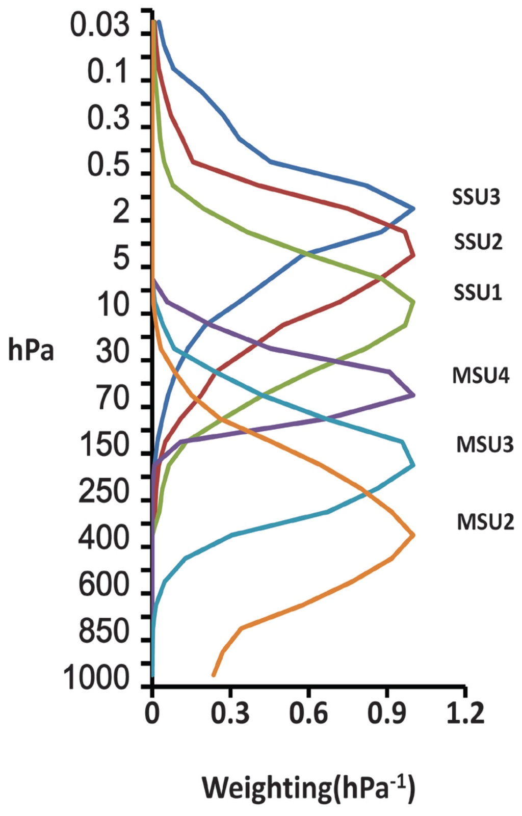
Figure 1. The weighting functions for the satellite Microwave Sounding Unit (MSU) and the Stratospheric Sounding Unit (SSU).

Figure 1. The weighting functions for the satellite Microwave Sounding Unit (MSU) and the Stratospheric Sounding Unit (SSU).

2.2. CMIP5 Simulations

We use the IPCC models at the Program for Climate Model Diagnosis and Intercomparison (PCMDI) [8]. The datasets used for this study are the historical run of 35 available models with 11 high-top models (model tops above 1 hPa), enabling the comparisons with the highest altitude SSU data for the period of 1979–2005. Table 1 lists information for all 35 models used in this study. Further details, together with access information, can be obtained at the following website [25]. The “historical” (HIS) run (1850–2005) is forced by past atmospheric composition changes (reflecting both anthropogenic and natural sources) including time evolving land cover. In addition, three types of experiments including pre-industrial control runs (PI), Greenhouse gases (GHG) only runs and natural forcing only (NAT) runs have been analyzed.

Table 1. The CMIP5/IPCC Data Sets and Selected Information.

IPCC I.D.	Pressure Level (hPa)	Center and Location	Forcing
CanESM2 CanCM4	1–1000	Canadian Centre for Climate Modelling and Analysis	GHG, SA, Oz, BC, OC, LU, Sl, Vl
HadGEM2-CC HadGEM2-AO HadGEM2-ES HadCM3	0.4–1000 10–1000	Met Office Hadley Centre	GHG, SA, Oz, BC, OC, LU, Sl, Vl
CESM1-WACCM CESM1-BGC CESM1-CAM5 CESM1-FASTCHEM CCSM4	0.4–1000 10–1000	NSF/DOE NCAR (National Center for Atmospheric Research) Boulder, CO, USA	Sl, GHG, Vl, SS, Ds, SD, BC, MD, OC, Oz, AA ,LU
MIROC-ESM-CHEM	0.03–1000	Japan Agency for Marine-Earth Science and Technology	GHG, SA, Oz, BC, OC, LU, Sl, Vl, MD
MIROC5	10–1000	Atmosphere and Ocean Research Institute, The University of Tokyo, Chiba, Japan National Institute for Environmental Studies, Ibaraki, Japan Japan Agency for Marine-Earth Science and Technology, Kanagawa, Japan	GHG, SA, Oz, LU, Sl, Vl, SS, Ds, BC, MD, OC
CMCC-CESM	0.01–1000	CMCC-Centro Euro-Mediterraneo peri Cambiamenti Climatici, Bologna, Italy	Nat, Ant, GHG, SA, Oz, Sl
MPI-ESM-LR MPI ESM-MR MPI-ESM-P	10–1000	Max Planck Institute for Meteorology	GHG, SD, Oz, LU, Sl, Vl
MRI-CGCM3 MRI-ESM1	0.4–1000	MRI (Meteorological Research Institute, Tsukuba, Japan)	GHG, SA, Oz, BC, OC, LU, Sl, Vl,
ACCESS1-0 ACCESS1-3	10–1000	Commonwealth Scientific and Industrial Research Organisation, Bureau of Meteorology, Australia	GHG, Oz, SA, Sl, Vl, BC, OC
BNU-ESM	10–1000	GCESS, BNU, Beijing, China	Nat, Ant
GISS-E2-H-CC GISS-E2-HGISS-E2-R-CC GISS-E2-R	10–1000	NASA Goddard Institute for Space Studies	GHG, LU, Sl, Vl, BC, OC, SA, Oz
IPSL-CM5A-LR IPSL-CM5B-LR IPSL-CM5B-MR	10–1000	Institut Pierre Simon Laplace, Paris, France	Nat, Ant, GHG, SA, Oz, LU, SS, Ds, BC, MD, OC, AA
NorESM1-M NorESM1-ME	10–1000	Norwegian Climate Centre	GHG, SA, Oz, Sl, Vl, BC, OC
inmcm4	10–1000	Institute for Numerical Mathematics, Moscow, Russia	N/A
CSIRO-Mk3-6-0	5–1000	Australian Commonwealth Scientific and Industrial Research Organization, Marine and Atmospheric Research, Queensland Climate Change Centre of Excellence	Ant, Nat (all forcings)
CNRM-CM5	10–1000	Centre National de Recherches Meteorologiques Centre Europeen de Recherches et de Formation Avancee en Calcul Scientifique	GHG, SA, Sl, Vl, BC, OC
FGOALS-g2	10–1000	Institute of Atmospheric Physics, Chinese Academy of Sciences, Tsinghua University	GHG, Oz, SA, BC, Ds, OC, SS, Sl, Vl

Notes: BC (black carbon); Ds (Dust); GHG (well-mixed greenhouse gases); LU (land-use change); MD (mineral dust); OC (organic carbon); Oz (tropospheric and stratospheric ozone); SA (anthropogenic sulfate aerosol direct and indirect effects); SD (anthropogenic sulfate aerosol, accounting only for direct effects); SI (anthropogenic sulfate aerosol, accounting only for indirect effects); Sl (solar irradiance); SO (stratospheric ozone); SS (sea salt); TO (tropospheric ozone); Vl (volcanic aerosol); Ant (anthropogenic forcing).

Table 1. The CMIP5/IPCC Data Sets and Selected Information.

IPCC I.D.	Pressure Level (hPa)	Center and Location	Forcing
CanESM2 CanCM4	1–1000	Canadian Centre for Climate Modelling and Analysis	GHG, SA, Oz, BC, OC, LU, Sl, Vl
HadGEM2-CC HadGEM2-AO HadGEM2-ES HadCM3	0.4–1000 10–1000	Met Office Hadley Centre	GHG, SA, Oz, BC, OC, LU, Sl, Vl
CESM1-WACCM CESM1-BGC CESM1-CAM5 CESM1-FASTCHEM CCSM4	0.4–1000 10–1000	NSF/DOE NCAR (National Center for Atmospheric Research) Boulder, CO, USA	Sl, GHG, Vl, SS, Ds, SD, BC, MD, OC, Oz, AA ,LU
MIROC-ESM-CHEM	0.03–1000	Japan Agency for Marine-Earth Science and Technology	GHG, SA, Oz, BC, OC, LU, Sl, Vl, MD
MIROC5	10–1000	Atmosphere and Ocean Research Institute, The University of Tokyo, Chiba, Japan National Institute for Environmental Studies, Ibaraki, Japan Japan Agency for Marine-Earth Science and Technology, Kanagawa, Japan	GHG, SA, Oz, LU, Sl, Vl, SS, Ds, BC, MD, OC
CMCC-CESM	0.01–1000	CMCC-Centro Euro-Mediterraneo peri Cambiamenti Climatici, Bologna, Italy	Nat, Ant, GHG, SA, Oz, Sl
MPI-ESM-LR MPI ESM-MR MPI-ESM-P	10–1000	Max Planck Institute for Meteorology	GHG, SD, Oz, LU, Sl, Vl
MRI-CGCM3 MRI-ESM1	0.4–1000	MRI (Meteorological Research Institute, Tsukuba, Japan)	GHG, SA, Oz, BC, OC, LU, Sl, Vl,
ACCESS1-0 ACCESS1-3	10–1000	Commonwealth Scientific and Industrial Research Organisation, Bureau of Meteorology, Australia	GHG, Oz, SA, Sl, Vl, BC, OC
BNU-ESM	10–1000	GCESS, BNU, Beijing, China	Nat, Ant
GISS-E2-H-CC GISS-E2-HGISS-E2-R-CC GISS-E2-R	10–1000	NASA Goddard Institute for Space Studies	GHG, LU, Sl, Vl, BC, OC, SA, Oz
IPSL-CM5A-LR IPSL-CM5B-LR IPSL-CM5B-MR	10–1000	Institut Pierre Simon Laplace, Paris, France	Nat, Ant, GHG, SA, Oz, LU, SS, Ds, BC, MD, OC, AA
NorESM1-M NorESM1-ME	10–1000	Norwegian Climate Centre	GHG, SA, Oz, Sl, Vl, BC, OC
inmcm4	10–1000	Institute for Numerical Mathematics, Moscow, Russia	N/A
CSIRO-Mk3-6-0	5–1000	Australian Commonwealth Scientific and Industrial Research Organization, Marine and Atmospheric Research, Queensland Climate Change Centre of Excellence	Ant, Nat (all forcings)
CNRM-CM5	10–1000	Centre National de Recherches Meteorologiques Centre Europeen de Recherches et de Formation Avancee en Calcul Scientifique	GHG, SA, Sl, Vl, BC, OC
FGOALS-g2	10–1000	Institute of Atmospheric Physics, Chinese Academy of Sciences, Tsinghua University	GHG, Oz, SA, BC, Ds, OC, SS, Sl, Vl

Notes: BC (black carbon); Ds (Dust); GHG (well-mixed greenhouse gases); LU (land-use change); MD (mineral dust); OC (organic carbon); Oz (tropospheric and stratospheric ozone); SA (anthropogenic sulfate aerosol direct and indirect effects); SD (anthropogenic sulfate aerosol, accounting only for direct effects); SI (anthropogenic sulfate aerosol, accounting only for indirect effects); Sl (solar irradiance); SO (stratospheric ozone); SS (sea salt); TO (tropospheric ozone); Vl (volcanic aerosol); Ant (anthropogenic forcing).

2.3. Methodology

To facilitate the inter-comparison study, all data are first interpolated to the same horizontal resolution of 5-degrees in longitude and latitude, then the temperature of the pressure levels in CMIP5 are converted to the equivalent brightness temperatures of the six SSU/MSU layers (SSU3, SSU2, SSU1, MSU4, MSU3, MSU2) based on the vertical weighting function of the SSU/MSU measurements in Figure 1 (the weighting functions were from the NOAA/STAR website). It is clear that only the 11 high-top models can be compared to the highest layers (SSU3, SSU2) of satellite data. Similar to the processing in the previous study [4], the six SSU/MSU channels represent the temperature for broad layer from the middle tropospheric MSU2 (peak at 6 km) to the upper stratospheric SSU3 (peak at 45 km).

Taylor’s [26] diagram and ratio of signal to noise are used to evaluate the performance of the models. The fitting of linear least squares is used to estimate the temperature trend. The model trend uncertainty is measured by the ensemble spread, which is defined by the standard deviation among CMIP5 climate model simulations. Multiple linear regression was performed for the analysis of model performance in stratosphere and troposphere.

3. Temporal Characteristics of Global Mean Temperature

3.1. Global Mean Temperature

Figure 2 shows the time series of global mean temperature anomalies of the satellite observations (thick blue line) and CMIP5 simulations at the SSU/MSU six layers. The SSU channel (Figure 2a–c) indicates cooling temperature trend at a rate of approximately −0.85 K/decade in the upper stratosphere (SSU3). MSU channel 4 (MSU4) shows −0.38 K/decade in the lower stratosphere (MSU4). It is clear that all three SSU and MSU4 channels demonstrate strong anomalies during the 1982–1983 and 1991–1992 periods, which is attributed to the volcanic eruptions of El Chichón (1982) and Mt. Pinatubo (1991).

In comparison, the troposphere (Figure 2e,f) shows a weak warming at a rate of +0.07 K/decade in MSU3, and +0.14 K/decade in the middle troposphere (MSU2).

For the CMIP5 simulations, all the models are able to capture the observed temperature variability in the upper and low stratosphere (Figure 2a–d) except some models demonstrate a larger, short-lived warming than observations due to the Mount Pinatubo volcano in 1991–1992. The overestimation of the temperature response is mainly due to the fact that the observed decreases in ozone concentrations following the major volcanic eruptions were not included in the forcing data set, which is why most models lead to overestimation of the stratospheric temperature response to volcanic eruptions, especially Pinatubo [11].

Figure 2. Global temperature anomalies time series (K) in the period of 1979–2005 at (a) SSU3, (b) SSU2; (c) SSU1. Note SSU1~SSU3 represent the SSU observational layers. Blue thick line represents the STAR observation. Gray and orange lines indicate the low-top and high-top CMIP5 model, respectively, Black thick line represents model ensemble mean. Figure 2b is the same as Figure 2a except for the MSU observation (d) MSU4; (e) MSU3; (f) MSU2. Note MSU2-MSU4 represents the MSU observational layers. MME is multiple model ensemble mean.

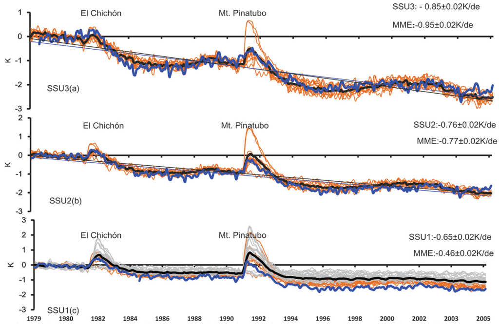
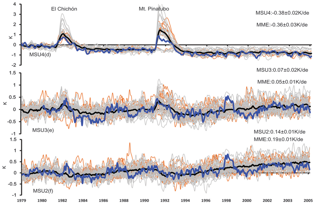
Figure 2. Global temperature anomalies time series (K) in the period of 1979–2005 at (a) SSU3, (b) SSU2; (c) SSU1. Note SSU1~SSU3 represent the SSU observational layers. Blue thick line represents the STAR observation. Gray and orange lines indicate the low-top and high-top CMIP5 model, respectively, Black thick line represents model ensemble mean. Figure 2b is the same as Figure 2a except for the MSU observation (d) MSU4; (e) MSU3; (f) MSU2. Note MSU2-MSU4 represents the MSU observational layers. MME is multiple model ensemble mean.

The model ensemble mean (MME: black thick line) is very similar to observations in the stratosphere. The major differences between the model ensemble mean and the observation is that the model ensemble mean overestimates the cooling in SSU3 channels and underestimates that in SSU1 where the difference reaches 0.19 K/decade. It should be noted that some models, IPSL-CM5A-LR, IPSL-CM5A-MR, IPSL-CM5B-LR, CMCC-CESM and INMCM4 even cannot reproduce strong volcanic eruptions anomalies in the stratosphere during the 1982–1983 and 1991–1992 periods, because they did not include volcanic aerosols.

In contrast, in the comparison of stratosphere, the CMIP5 models show an obvious discrepancy from the MSU observations (Figure 2e,f) where the multi-model ensemble mean cannot produce the temperature variability. Some models even show an opposite phase of variability to the MSU observations, but there is no large difference in the global mean temperature trend between models and observations.

3.2. Consistencies between Simulations and Observations

The evaluation of the global mean temperatures in CMIP5 simulations in comparison with the SSU/MSU observations is accomplished through the Taylor-diagram. The Taylor diagram is a convenient way of evaluating different model’s performance with observation using three related parameters: correlation with observed data, centered root-mean-square (RMS), and standard deviation. Models with as much variance as the observations’ largest correlation and with the least RMS error are considered best performers in the Taylor diagram. In the stratosphere (Figure 3), the correlation coefficient between SSU/MSU and CMIP5 climate models have a large value ranging from 0.60 in the lower stratosphere to 0.95 in the middle to upper stratosphere. This reflects the strong consistency in the global mean stratospheric temperature between the CMIP5 climate model simulations and observation. The results showed that the 11 high-top models (triangle symbol) have higher correlation coefficients and a more centralized distribution than the low-top models in the low stratosphere. It is worth noting that the high-top model CMCC-CESM does not include volcanic aerosol in the stratosphere during the 1982–1983 and 1991–1992 periods, but the high correlation coefficient in SSU3, SSU2, SSU1 and MSU4 indicated the better agreement with observation in the stratosphere, which is totally different from the poor simulations in the low top model discovered in many previous studies [27,28,29]. It is obvious that the model lid height plays a very crucial role in the simulation of stratospheric temperature variability.

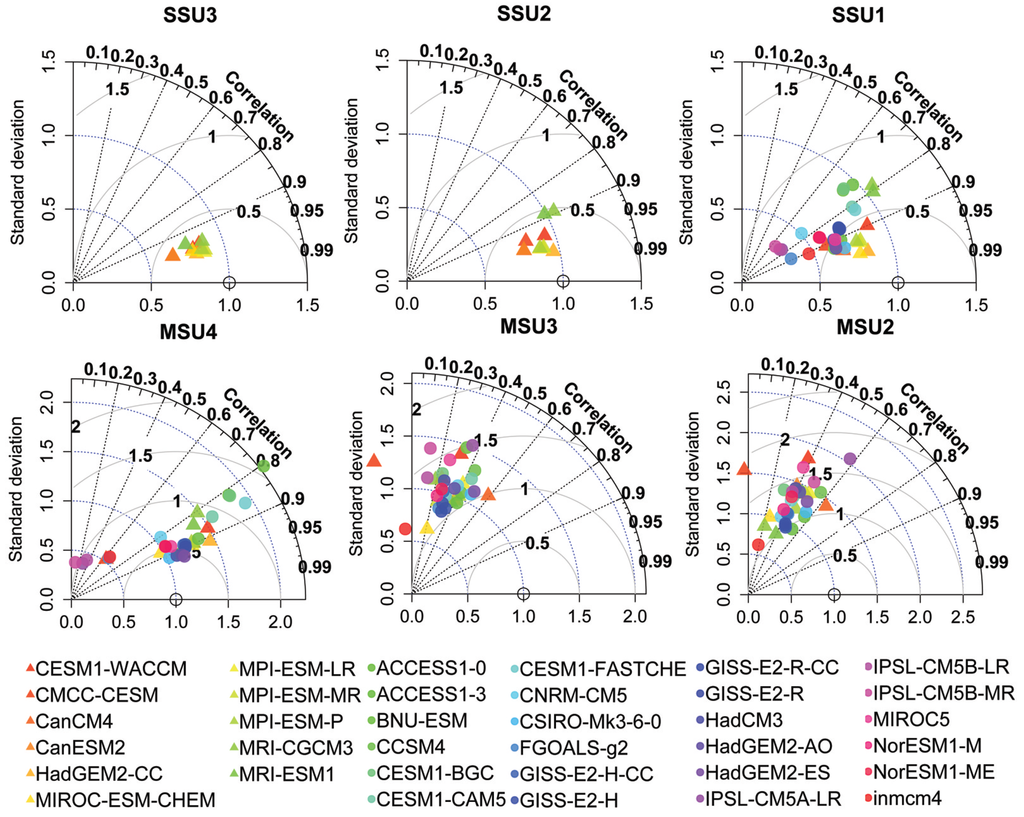
Figure 3. Taylor diagram for time series of observed and simulated global mean temperature. Normalized Standard deviation, Correlation coefficient, and The Root Mean Squared Deviation (RMSD) are presented in one diagram. An ideal model has a standard deviation ratio of 1.0 and a correlation coefficient of 1.0. Triangle symbols represent high-top models (correlations greater than 0.14 are statistically significant at the 99% confidence level).

Figure 3. Taylor diagram for time series of observed and simulated global mean temperature. Normalized Standard deviation, Correlation coefficient, and The Root Mean Squared Deviation (RMSD) are presented in one diagram. An ideal model has a standard deviation ratio of 1.0 and a correlation coefficient of 1.0. Triangle symbols represent high-top models (correlations greater than 0.14 are statistically significant at the 99% confidence level).

In contrast, the correlations of the CMIP5 model simulations with the MSU observations in the troposphere are sharply reduced. This demonstrates a lower correlation with the MSU in the CMIP5 simulations, which indicates that the CMIP5 simulations in the troposphere are in worse agreement than those in the stratosphere. The model CMCC-CESM shows a negative correlation with the MSU observations in the two MSU channels, and CanCM4 model simulations in the troposphere show much better agreement in the troposphere than their counterpart climate models. Additionally, models have a more centralized distribution in the stratosphere than troposphere implying that most of the models have better agreement in the stratosphere.

Results from the Taylor diagram suggest that models show better agreement with observation and smaller intermodel discrepancy in the stratosphere than in the troposphere, especially for the high-top models. The lower correlation in the troposphere is generally because the temperature variations in the troposphere demonstrate mostly unforced internal variability, and free-running coupled-ocean-atmosphere models will never capture the timing of that variability. Further research is therefore needed to understand the forcing of internal variability and the principle of the coupled ocean–atmosphere system to improve the performance of the CMIP5 models in the troposphere.

3.3. Uncertainty Analysis in Model Simulations

To quantitatively reveal the spread and convergence of the climate models in reproducing the Stratospheric and Tropospheric Temperature, the signal-to-noise ratio is evaluated using the method of Zhou [30].

Ensemble mean is given by the ensemble average of all model simulations, that is

$$x_e\left(t\right)=\frac{1}{N}{\displaystyle \sum }_{n=1}^{N}x\left(n,t\right)$$

(1)

where N is the total number of models, x is the global mean time series, x(n, t) represents the simulation of nth model at year t of a time length T. Climatological mean is defined by σ_e.

$$x_c=\frac{1}{NT}{\displaystyle \sum }_{n=1}^N{\displaystyle \sum }_{t=1}^{T}x\left(n,t\right)=\frac{1}{T}{\displaystyle \sum }_{t=1}^T{x}_e\left(t\right)$$

(2)

The standard deviation of the x_e (t) is used to measure modelled temperature trends in response to external signal. The dispersion of the simulation (measured by σ_i the standard deviation of x(n, t)) indicates intermodel variability, which is noise for the climate reproduction. From the definition of the two averages, we have

$${\sigma }_e^2=\frac{1}{T}{\displaystyle \sum }_{t=1}^T{\left[x_e \left(t\right)-x_c\right]}^2$$

(3)

$${\sigma }_i^2=\frac{1}{T}{\displaystyle \sum _{t=1}^T\left\{\frac{1}{N}{\displaystyle \sum _{n=1}^N{\left[x\left(n,t\right)-x_e\left(t\right)\right]}^2}\right\}}$$

(4)

The signal to noise ratio (S/N) is defined as S/N = λ = $\frac{{\sigma }_e^2}{{\sigma }_i^2}$.

Here we compute that S/N ratio for the period of 1979–2005 from stratosphere to troposphere. Analysis of S/N (Table 2) indicates that the stratosphere stands out as having much higher S/N (3.53–57.98) than the troposphere (0.48–1.36), where the forced signal is much larger than intermodal noise, especially for SSU3. The S/N ratio reduced sharply from SSU2 (28.31) to SSU1 (5.26), which is partially due to the inclusion of low-top models increasing intermodal noise.

Table 2. Signal-to-noise ratio (S/N) for stratospheric and tropospheric air temperature.

Layer	SSU3	SSU2	SSU1	MSU4	MSU3	MSU2
S/N	57.98	28.31	5.26	3.53	0.48	1.36

Table 2. Signal-to-noise ratio (S/N) for stratospheric and tropospheric air temperature.

Layer	SSU3	SSU2	SSU1	MSU4	MSU3	MSU2
S/N	57.98	28.31	5.26	3.53	0.48	1.36

3.4. Trend Changes with Vertical Level

The vertical profile of the global mean temperature trends shows (Figure 4) that the CMIP5 model’s (Figure 4a) temperature trend cooling rates in the upper stratosphere are less than the SSU observations, especially in the SSU1 channel. Also, the low-top models further underestimate the cooling trend than the high-top models in the stratosphere.

The crossover points identify a transition from tropospheric warming to stratospheric cooling. It is obvious that the most of the low-top models are higher than the corresponding crossover point from the MSU observations and high-top models. On the other hand, the ensemble spread among the CMIP5 model simulations (Figure 4b) is generally between 0.04 and 0.1 K/decade from the middle troposphere to the upper stratosphere, with the maximum spread appearing at the point of the SSU1 level, which is mainly due to the low-top models.

The above results clearly show that high-top models have better consistency with the SSU/MSU observations than low-top models in global mean temperature variability.

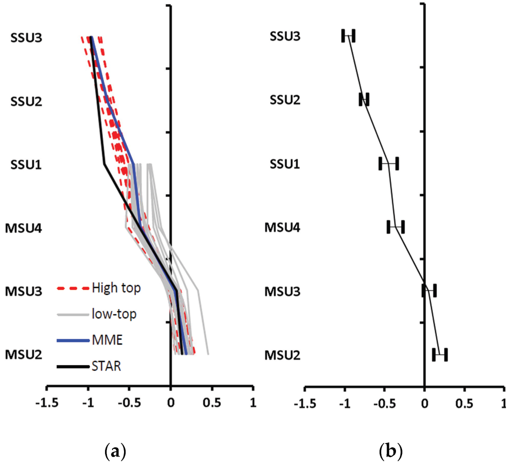
Figure 4. Vertical profile of global mean temperature trends and spread among the data sets for CMIP5 model simulations. Note SSU1-3 and MSU2-4 represent the SSU/MSU observational layers (unit K/decade). (a) Vertical profile temperature trends; (b) spread among models.

Figure 4. Vertical profile of global mean temperature trends and spread among the data sets for CMIP5 model simulations. Note SSU1-3 and MSU2-4 represent the SSU/MSU observational layers (unit K/decade). (a) Vertical profile temperature trends; (b) spread among models.

4. Spatial Pattern of Temperature Trends

4.1. Trend Changes with Latitude

To better understand the spatial pattern of the CMIP5 model simulations, the latitude profiles of the temperature trend have been plotted to facilitate comparing the differences between the datasets. The results indicate (Figure 5) that the linear trends are highly sensitive to the latitude of interest. All exhibit predominant cooling in the stratosphere and warming in the troposphere except for the southern high latitudes. Also, there is an extremely strong cooling trend in the three SSU channel observations over the tropics and arctic.

For the upper stratosphere (Figure 5a–c), a distinguishing difference in the CMIP5 simulations from SSU observations is found over the tropics, where the cooling rates get up to −1.2 K/decade in the SSU2 layer (Figure 5b). This is approximately −0.5 K/decade lower than the value in the CMIP5 models. In addition, the cooling trend shows a sharp gradient from high to low latitude in the SSU observations.

For the layer from the middle troposphere to the lower stratosphere (Figure 5d–f), the MSU data shows a consistent trend with the CMIP5 models, except some models show more cooling than that observed at MSU4 over Antarctica. An important fact worth noting is that cooling was found in the troposphere over Antarctica, with the maximum cooling trend being approximately −1.8 K/decade in the upper troposphere. At the same time, warming trends have been observed over the tropics and the whole Northern hemisphere. This layer also displayed a substantial temperature difference between the Antarctic and the rest of the areas.

It is obvious that the cooling trends of the stratospheric temperature change markedly with latitude and the largest trend is found in the tropical and arctic latitudes. In contrast, the warming trend increases with latitude from south to north in the troposphere, but the spread retains a small value except for both polar areas. Conversely, the south to north latitudinal cooling trend in the stratosphere decreased. To a first order (linear), the tropospheric warming by latitude is offset by stronger latitudinal cooling in the stratosphere indicating the atmosphere is adjusting to surface and tropospheric heating to maintain radiative balance.

Figure 5. Temperature trend change with latitude for the layers (a) SSU3; (b) SSU2; (c) SSU1; (d) MSU4; (e) MSU3; (f) MSU2. Note SSU1~3 and MSU2~4 represent the SSU/MSU observational layers. Heavy black line indicates the SSU/MSU observation, gray and red thin lines represent the low-top and high top CMIP5 model, respectively.

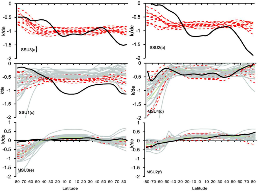
Figure 5. Temperature trend change with latitude for the layers (a) SSU3; (b) SSU2; (c) SSU1; (d) MSU4; (e) MSU3; (f) MSU2. Note SSU1~3 and MSU2~4 represent the SSU/MSU observational layers. Heavy black line indicates the SSU/MSU observation, gray and red thin lines represent the low-top and high top CMIP5 model, respectively.

4.2. Distribution of Longitude-Latitude Trend Spread

Figure 6 displays the latitudinal-longitudinal variation of global temperature trend spreads for 1979–2005 for the layers from the middle troposphere (6 km height) to the upper stratosphere (45 km height). The results indicate (Figure 6) that the spreads are highly sensitive to the latitude of interest, from 0.05 K/decade in tropical and subtropical areas to 0.5 K/decade in the southern polar region. The largest layer spread locations change with vertical level; the largest spread in the lower stratosphere (SSU1, MSU4) exceeds 0.5 K/decade over Antarctic areas, which is mainly due to some models significantly overestimating the cooling.

In contrast, there are some remarkable discrepancies in the tropical regions in the MSU4 layer, especially in the central Pacific region. It is worth noting that the spread of the CMIP5 simulations in the middle troposphere (MSU2) remains a relatively small value at all latitudes. The smaller spread in the MSU2 reflects the high consistency at all latitudes in CMIP5 simulations.

To summarize, the cooling trends of the stratospheric temperature markedly change with latitude, and the largest trend is found in the tropics-subtropics but the largest spread is found in the South Polar Region. In contrast, the warming trend increases with latitude from south to north in the troposphere, but the spread retains a small value except for both polar areas. Conversely, the cooling trend decreases with latitude from south to north in the stratosphere consistent with latitudinal radiative balance.

Figure 6. Spatial distribution of spread of temperature trends in CMIP5 model simulations. Note SSU1-3 and MSU2-4 represent the SSU/MSU observational layers (unit K/de).

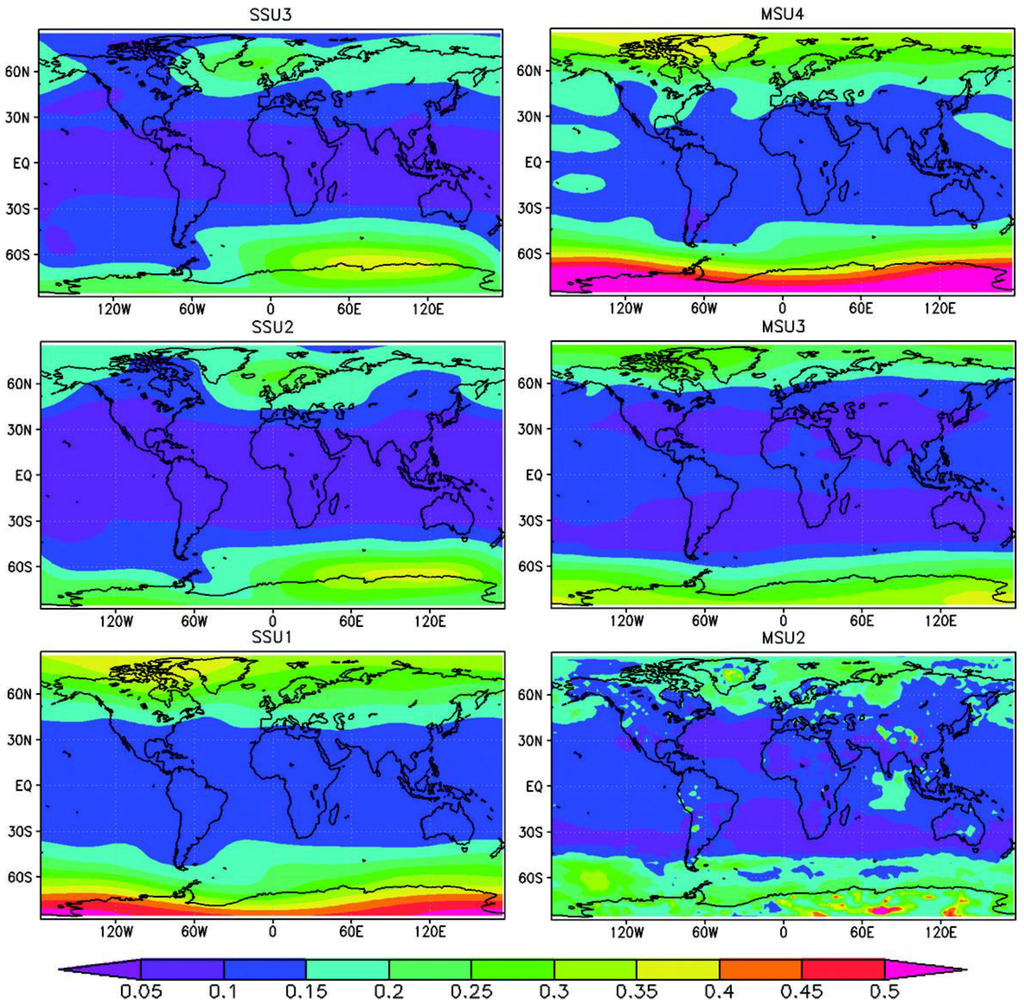
Figure 6. Spatial distribution of spread of temperature trends in CMIP5 model simulations. Note SSU1-3 and MSU2-4 represent the SSU/MSU observational layers (unit K/de).

5. Discussion

According to the above analysis, there is one point worth noting. All selected CMIP5 models showed a much higher correlation with SSU/MSU observations and higher intermodal consistency in the stratosphere compared to the global mean temperature in the troposphere.

In order to understand the possible reasons for the difference between the stratosphere and troposphere, the model's response to different forcings and their internal variability are investigated. In particular, three types of simulations are analyzed: pre-industrial control runs (piControl: PI), Greenhouse gases (GHG) only runs and natural forcing only (historicalNat: NAT) runs. Only two out of the 11 high-top models MIROC-ESM-CHEM and the MRI-CGCM3 included all three types of simulations and thus are analyzed here.

The time series of global mean temperature anomalies for SSU3 and MSU2 observational layers in GHG-only experiment, natural-only forcing run and preindustrial control run are shown in Figure 7. In SSU3, there is no significant trend in the natural-only forcing run and preindustrial control run, stratospheric cooling can only be reproduced in the model with anthropogenic forcing. Both models underestimated the cooling in the GHG-only experiment (0.91 ± 0.02 K/de) compared to all-forcing historical simulation (MRI-CGCM3 0.98 ± 0.02 K/de and MIROC-ESM-CHEM 0.96 ± 0.02 K/de) (ozone forcing is not included due to the dataset being unavailable). Solar variability and volcanic eruptions can be easily found in the natural-only forcing run. Similar results can be obtained in other stratospheric observation layers (Figure 8).

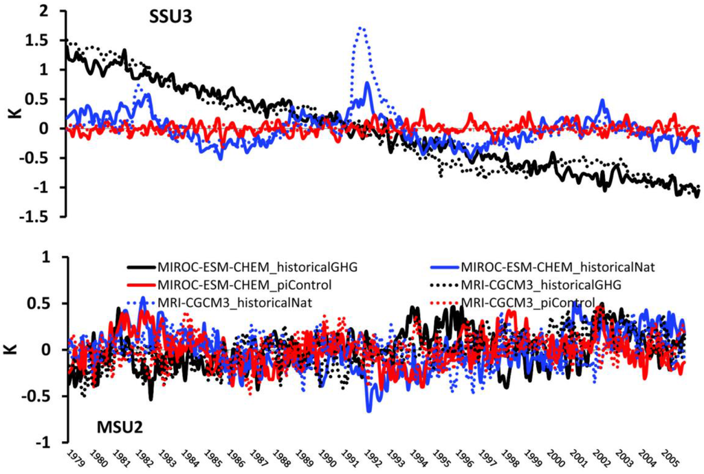
Figure 7. Global mean temperature anomalies for SSU3 and MSU2 observational layers in GHG-only historical experiment, Natural-only forcing run and preindustrial control run.

Figure 7. Global mean temperature anomalies for SSU3 and MSU2 observational layers in GHG-only historical experiment, Natural-only forcing run and preindustrial control run.

In comparison, the warming trend only can be detected from the GHG-only experiment, but the difference in the trend (MRI-CGCM3 0.15 ± 0.02 K/de and MIROC-ESM-CHEM 0.09 ± 0.03 K/de)is bigger compared to simulation results from SSU3, and also no significant trend in natural-only forcing run and preindustrial control run was observed.

To quantitatively link the different model performances in the stratosphere and troposphere with the internal variability of the climate model and the model response to a given external forcing, a multiple linear regression analyses [31] were performed for the all forcing historical runs using the GHG-only experiment, natural-only forcing run and preindustrial control run as regressors. Multiple linear regression attempts were made to model the relationship between two or more explanatory variables and a response variable by fitting a linear equation.

$$\text{Y}=b_{0+}{b}_1{X}_1+b_2{X}_2+\cdots +b_p{X}_p$$

(5)

Y is the dependent variable, (x1, x2 … xp) is a set of p explanatory variables. ${\text{b}}_0$ is the constant term and ${\text{b}}_1$ to ${\text{b}}_{\text{p}}$ are the coefficients relating the p explanatory variables. A regression coefficient which is significantly greater than zero indicates a detectable response to the forcing concerned. Here, we assume that model output may be written as a linear sum of the simulated responses to individual forcing (GHG, NAT) and internal variability, each scaled by a regression coefficient plus residual variability.

The regression coefficients are shown in Figure 9. The multiple linear regression results with GHG, NAT and PI can accurately reproduce the amplitude and phase of historical runs in the stratosphere (Figure 10). In the troposphere, the multiple linear regression results have their own amplitude and phase variability which does not match historical runs in any detail.

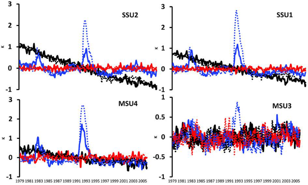
Figure 8. Same as Figure 7 except for MSU4, MSU3, SSU2, and SSU1.

Figure 8. Same as Figure 7 except for MSU4, MSU3, SSU2, and SSU1.

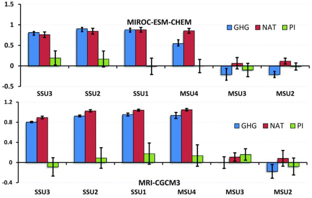
Figure 9. Regression coefficients derived from the regression of historical global mean temperatures’ time series with greenhouse gases forced run (GHG) natural forced run (NAT) and pre-industrial control run (PI) (error bar: 95% confidence intervals for the coefficient estimates).

Figure 9. Regression coefficients derived from the regression of historical global mean temperatures’ time series with greenhouse gases forced run (GHG) natural forced run (NAT) and pre-industrial control run (PI) (error bar: 95% confidence intervals for the coefficient estimates).

The results suggest that the stratospheric temperature is dominated by external forcing and response [32]. This is different to the troposphere where the temperature variability is driven by both internal variability and external forcing, and the model response to external forcing is nonlinear.

That is why all selected CMIP5 models showed a much higher correlation with SSU/MSU observations and higher intermodal consistency in the stratosphere compared to the global mean temperature in the troposphere.

According to the above analysis, a final important point to emphasize is that all selected CMIP5 model simulations showed high correlation with SSU/MSU observations in the stratosphere compared to the global mean temperature in the troposphere, but these models failed to reproduce the latitude-longitude pattern of the temperature trends. On the other hand, most of the CMIP5 models do not have some of the necessary physical processes. For example, most of the selected CMIP5 models do not include a chemistry model in the stratosphere; only the MIROC-ESM-CHEM and CESM1-WACCM includes chemistry and the chemistry model was recognized as a very important component to reproduce the true atmosphere [33,34].

Figure 10. Global mean temperature anomalies simulated by MRI-CGCM3 at SSU1-SSU3 and MSU2-4. Red dash line represents the historical run (Hist). Blue line indicates the multiple linear regression results (Reg) with greenhouse gases forced run (GHG) natural forced run (NAT) and pre-industrial control run (PI).

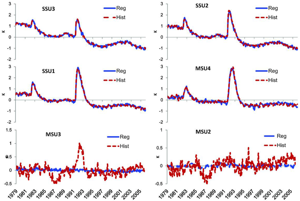
Figure 10. Global mean temperature anomalies simulated by MRI-CGCM3 at SSU1-SSU3 and MSU2-4. Red dash line represents the historical run (Hist). Blue line indicates the multiple linear regression results (Reg) with greenhouse gases forced run (GHG) natural forced run (NAT) and pre-industrial control run (PI).

6. Conclusions

Based on the satellite SSU and MSU temperature observations from 1979 through 2005, the trends and uncertainties in CMIP5 model simulations from the middle troposphere to the upper stratosphere (5–50 km) have been examined. The results are summarized as follows:

The CMIP5 model simulations reproduced a common feature with cooling in the stratosphere and warming in the troposphere, but the trend exhibits a remarkable discrepancy among the selected models. The cooling rate is higher than the SSU3 measurements at the upper stratosphere and less than SSU at the lower stratosphere.

Regarding the temporal variation of the global mean temperature, the CMIP5 model simulations significantly reproduced the volcanic signal and were highly correlated with the SSU measurements in the upper stratosphere during the study period. However, these models have lower temporal correlation with observations in the middle-upper troposphere.

Regarding the regional variation of the global temperature trends, the CMIP5 simulations displayed a different latitudinal pattern compared to the SSU/MSU measurements in all six layers from the middle troposphere to the upper stratosphere.

Generally, the high-top models show better agreement with observations than the low-top model, especially in the lower stratosphere. The temperature trends and spread show marked changes with latitude; the greatest cooling is found in the tropics in the upper stratosphere and the greatest warming appears in the Arctic in the middle troposphere. The CMIP5 simulations underestimated the stratospheric cooling in the tropics compared to the SSU observations and remarkably overestimated the cooling in the Antarctic from the upper troposphere to the lower stratosphere (MSU3-SSU3). The largest trend spread among the CMIP5 simulations is seen in both the Arctic and Antarctic in the stratosphere and troposphere, and the CMIP5 simulations retain similar spread values in the tropics in both the troposphere and stratosphere.

References

- Eichelberger, S.J.; Hartmann, D.L. Changes in the strength of the brewer–dobson circulation in a simple AGCM. Geophys. Res. Lett. 2005, 32, L15807. [Google Scholar] [CrossRef]
- Cordero, E.C.; Forster, P.M. Stratospheric variability and trends in models used for the IPCC AR4. Atmos. Chem. Phys. 2006, 6, 5369–5380. [Google Scholar] [CrossRef]
- Seidel, D.J.; Angell, J.K.; Christy, J.; Free, M.; Klein, S.A.; Lanzante, J.R.; Mears, C.; Parker, D.; Schabel, M.; Spencer, R.; et al. Uncertainty in signals of large-scale climate variations in radiosonde and satellite upper-air temperature datasets. J. Clim. 2004, 17, 2225–2240. [Google Scholar] [CrossRef]
- Seidel, D.J.; Gillett, N.P.; Lanzante, J.R.; Shine, K.P.; Thorne, P.W. Stratospheric temperature trends: Our evolving understanding. Wiley Interdiscip. Rev. Clim. Chang. 2011, 2, 592–616. [Google Scholar] [CrossRef]
- Young, P.J.; Thompson, D.W.J.; Rosenlof, K.H.; Solomon, S.; Lamarque, J. The seasonal cycle and interannual variability in stratospheric temperatures and links to the brewer–dobson circulation: An analysis of MSU and SSU Data. J. Clim. 2011, 24, 6243–6258. [Google Scholar] [CrossRef]
- Xu, J.; Powell, A. Ensemble spread and its implication for the evaluation of temperature trends from multiple radiosondes and reanalyses products. Geophys. Res. Lett. 2010, 37, L17704. [Google Scholar] [CrossRef]
- Xu, J.; Powell, A. Uncertainty estimation of the global temperature trends for multiple radiosondes, reanalyses, and CMIP3/IPCC climate model simulations. Theor. Appl. Climatol. 2012, 108, 505–518. [Google Scholar] [CrossRef]
- Jiang, Z.; Li, W.; Xu, J.; Li, L. Extreme precipitation indices over China in CMIP5 models. Part I: Model evaluation. J. Clim. 2015, 28, 8603–8619. [Google Scholar] [CrossRef]
- Cai, J.; Xu, J.; Powell, A.; Guan, Z.; Li, L. Intercomparison of the temperature contrast between the arctic and equator in the pre- and post periods of the 1976/1977 regime shift. Theor. Appl. Climatol. 2015. [Google Scholar] [CrossRef]
- Taylor, K.E.; Stouffer, R.J.; Meehl, G.A. An overview of CMIP5 and the experiment design. Bull. Am. Meteor. Soc. 2012, 93, 485–498. [Google Scholar] [CrossRef]
- Charlton-Perez, A.J.; Baldwin, M.P.; Birner, T. On the lack of stratospheric dynamical variability in low-top versions of the CMIP5 models. J. Geophys. Res. Atmos. 2013, 118, 2494–2505. [Google Scholar] [CrossRef]
- Thompson, D.W.J.; Seidel, D.J.; Randel, W.J.; Zou, C.Z.; Butler, A.H.; Mears, C.; Osso, A.; Long, C.; Lin, R. The mystery of recent stratospheric temperature trends. Nature 2012, 491, 692–697. [Google Scholar] [CrossRef] [PubMed]
- Santer, B.D.; Painter, J.F.; Bonfils, C.; Mears, C.A. Identifying human influences on atmospheric temperature. Proc. Natl. Acad. Sci. USA 2012, 110, 26–33. [Google Scholar] [CrossRef] [PubMed]
- Santer, B.D.; Painter, J.F.; Bonfils, C.; Mears, C.A. Human and natural influences on the changing thermal structure of the atmosphere. Proc. Natl Acad. Sci. USA 2013, 110, 17235–17240. [Google Scholar] [CrossRef] [PubMed]
- Christy, J.R.; Spencer, R.W.; Braswell, W.D. MSU tropospheric temperatures: Dataset construction and radiosonde comparisons. J. Atmos. Oceanic Technol. 2000, 17, 1153–1170. [Google Scholar] [CrossRef]
- Mears, C.A.; Schabel, M.C.; Wentz, F.J. A reanalysis of the MSU channel 2 tropospheric temperature record. J. Clim. 2003, 16, 3650–3664. [Google Scholar] [CrossRef]
- Zou, C.; Goldberg, M.; Cheng, Z.; Grody, N.; Sullivan, J.; Cao, C.; Tarpley, D. Recalibration of microwave sounding unit for climate studies using simultaneous nadir overpasses. J. Geophys. Res. 2006, 111, D19114. [Google Scholar] [CrossRef]
- Zou, C.Z.; Qian, H.F.; Wang, W.H. Recalibration and merging of SSU observations for stratospheric temperature trend studies. J. Geophys. Res.: Atmos. 2014, 119, JD021603. [Google Scholar] [CrossRef]
- Wang, W.H.; Zou, C.Z. AMSU-A-Only atmospheric temperature data records from the lower troposphere to the top of the stratosphere. J. Atmos. Oceanic Technol. 2014, 31, 808–825. [Google Scholar] [CrossRef]
- Santer, B.D.; Hnilo, J.J.; Wigley, T.M.L.; Boyle, J.S.; Doutriaux, C.; Fiorino, M.; Parker, D.E.; Taylor, K.E. Uncertainties in observationally based estimates of temperature change in the free atmosphere. J. Geophys. Res. 1999, 104, 6305–6333. [Google Scholar] [CrossRef]
- Wang, L.; Zou, C.Z.; Qian, H. Construction of stratospheric temperature data records from stratospheric sounding units. J. Clim. 2012, 25, 2931–2946. [Google Scholar] [CrossRef]
- Keckhut, P.; Randel, W.J.; Claud, C.; Leblanc, T.; Steinbrecht, W.; Funatsu, B.M. Tidal effects on stratospheric temperature series derived from successive advanced microwave sounding units. Q. J. R. Meteorol. Soc. 2014, 141, 477–483. [Google Scholar] [CrossRef] [PubMed]
- Nash, J.; Forrester, G.F. Long-term monitoring of stratospheric temperature trends using radiance measurements obtained by the TIROS-N series of NOAA spacecraft. Adv. Sp. Res. 1986, 6, 37–44. [Google Scholar] [CrossRef]
- Shine, K.P.; Barnett, J.J.; Randel, W.J. Temperature trends derived from stratospheric sounding unit radiances: The effect of increasing CO2 on the weighting function. Geophys. Res. Lett. 2008, 35, L02710. [Google Scholar] [CrossRef]
- Detail Information about CMIP5 Model. Available online: http: //cmip -pcmdi. llnl. gov/cmip5 (accessed on 21 December 2015).
- Taylor, K.E. Summarizing multiple aspects of model performance in a single diagram. J. Geophys. Res. 2001, 106, 7183–7192. [Google Scholar] [CrossRef]
- Cagnazzo, C.; Manzini, E. Impact of the Stratosphere on the winter tropopospheric teleconnections between ENSO and the North-Atlantic European region. J. Clim. 2009, 22, 1223–1238. [Google Scholar] [CrossRef]
- Hardiman, S.C.; Butchart, N.; Hinton, T.J.; Osprey, S.M.; Gray, L.J. The effect of a well-resolved stratosphere on surface climate: Differences between CMIP5 simulations with high and low top versions of the met office climate model. J. Clim. 2012, 25, 7083–7099. [Google Scholar] [CrossRef]
- Shaw, T.A.; Perlwitz, J. The impact of stratospheric model configuration on planetary scale waves in northern hemisphere winter. J. Clim. 2010, 22, 3369–3389. [Google Scholar] [CrossRef]
- Zhou, T.; Yu, R. Twentieth-century surface air temperature over China and the globe simulated by coupled climate models. J. Clim. 2006, 19, 5843–5858. [Google Scholar] [CrossRef]
- Gillett, N.P.; Akiyoshi, H.; Bekki, S.; Braesicke, P.; Eyring, V.; Garcia, R.R.; Karpechko, A.Y. Attribution of observed changes in stratospheric ozone and temperature. Atmos. Chem. Phys. 2011, 11, 599–609. [Google Scholar] [CrossRef]
- McLandress, C.; Jonsson, A.I.; Plummer, D.A.; Reader, M.C.; Scinocca, J.F.; Shepherd, T.G. Separating the effects of climate change and ozone depletion. Part 1: Southern Hemisphere stratosphere. J. Clim. 2010, 23, 5002–5020. [Google Scholar] [CrossRef]
- Guo, D.; Su, Y.; Shi, C.; Xu, J.; Powell, A.M. Double core of ozone valley over the Tibetan plateau and its possible mechanisms. J. Atmos. Sol. Terr. Phys. 2015, 130, 127–131. [Google Scholar] [CrossRef]
- Meehl, G.A.; Arblaster, J.M.; Matthes, K.; Sassi, F.; Loon, H. Amplifying the Pacific climate system response to a small 11-year solar cycle forcing. Science 2009. [Google Scholar] [CrossRef] [PubMed]
© 2015 by the authors; licensee MDPI, Basel, Switzerland. This article is an open access article distributed under the terms and conditions of the Creative Commons by Attribution (CC-BY) license (http://creativecommons.org/licenses/by/4.0/).