Article

Mapping Aquatic Vegetation in a Tropical Wetland Using High Spatial Resolution Multispectral Satellite Imagery

by
Timothy G. Whiteside
* and
Renée E. Bartolo
Environmental Research Institute of the Supervising Scientist, PO Box 261, Darwin, NT 0801, Australia
*
Author to whom correspondence should be addressed.
Remote Sens. 2015, 7(9), 11664-11694; https://doi.org/10.3390/rs70911664
Submission received: 3 March 2015 / Revised: 14 August 2015 / Accepted: 1 September 2015 / Published: 11 September 2015

Abstract

:
Vegetation plays a key role in the environmental function of wetlands. The Ramsar-listed wetlands of the Magela Creek floodplain in Northern Australia are identified as being at risk from weeds, fire and climate change. In addition, the floodplain is a downstream receiving environment for the Ranger Uranium Mine. Accurate methods for mapping wetland vegetation are required to provide contemporary baselines of annual vegetation dynamics on the floodplain to assist with analysing any potential change during and after minesite rehabilitation. The aim of this study was to develop and test the applicability of geographic object-based image analysis including decision tree classification to classify WorldView-2 imagery and LiDAR-derived ancillary data to map the aquatic vegetation communities of the Magela Creek floodplain. Results of the decision tree classification were compared against a Random Forests classification. The resulting maps showed the 12 major vegetation communities that exist on the Magela Creek floodplain and their distribution for May 2010. The decision tree classification method provided an overall accuracy of 78% which was significantly higher than the overall accuracy of the Random Forests classification (67%). Most of the error in both classifications was associated with confusion between spectrally similar classes dominated by grasses, such as Hymenachne and Pseudoraphis. In addition, the extent of the sedge Eleocharis was under-estimated in both cases. This suggests the method could be useful for mapping wetlands where statistical-based supervised classifications have achieved less than satisfactory results. Based upon the results, the decision tree method will form part of an ongoing operational monitoring program.

Graphical Abstract

1. Introduction

Vegetation is a vital component, and plays an important role in the environmental function, of wetland ecosystems [1]. The mapping and monitoring of vegetation status are key technical tasks required for the sustainable management of wetland ecosystems. In addition, detectable changes in vegetation structure and distribution in wetlands may be indicators of system change which maybe natural or the result of degradation. Satellite multispectral imagery can be used to detect the spectral characteristics of features on the Earth’s surface which in turn can be linked to bio-physical parameters of the region under investigation. Remote sensing has been a popular tool for mapping wetlands [2,3] and has advantages over field-based techniques, which can be resource intensive and problematic when the study area is remote and hazardous.
There have been a number of recent reviews of remote sensing of wetlands [2,4,5,6]. Remote sensing examples show that Landsat imagery has been used to successfully map many wetlands across the planet [7,8,9]. Aerial photography has been used to map wetlands with success, and despite the limited spectral information, is the preferred option for some researchers over moderate resolution satellite imagery such as Landsat. The finer spatial resolution of aerial photography enables the detection of features and classification of a large number of classes [5,10,11]. Synthetic aperture radar (SAR) data has also been used to map wetland vegetation and is often preferred due to the sensitivity of microwave energy to soil moisture and its ability to penetrate vegetative canopies [4]. L-band SAR data has been successful in discriminating inundated areas that are vegetated, such as Melaleuca swamps [12]. In addition, the fusion of optical and radar data has been shown to be effective in mapping long term vegetation and inundation dynamics of tropical floodplains [12].
The optical remote sensing of wetland vegetation can be problematic. For example, medium spatial resolution (MSR) imagery (with pixels with a ground sample distance (GSD) of 10–30 m), such as Landsat TM data, have proven insufficient for discriminating vegetation species in detailed wetland environments [10,13,14]. According to Adam et al. [2], MSR imagery is spatially and spectrally too coarse to distinguish the fine ecological divisions and gradients between vegetation units in wetland ecosystems. Boyden et al. [9] identified a number of challenges for remote sensing of monsoonal wetland environments, mostly associated with the highly variable annual rainfall and subsequent variation in water extent and levels within the floodplain. The use of high spatial resolution (HSR) multispectral satellite data (GSD < 5 m) should address the issues raised by Adam et al. [2]. However, HSR data displays greater within-class spectral variability than MSR data, and consequently, it is more difficult to discriminate spectrally mixed land covers using per-pixel classifications.
To reduce the spurious classification of pixels in HSR imagery, geographical object-based image analysis (GEOBIA) methods are widely used [15,16], whereby imagery is initially segmented into homogenous image objects that reflect spatial patterns in the imagery prior to classification. While the concepts of image segmentation and object classification have been around for several decades [17], the emergence of robust object-oriented approaches to the automated classification of satellite imagery appears to be one of the major advances in image processing in the last ten years [18]. GEOBIA has recently been identified as a paradigm [15] and is finding increasing popularity particularly when applied to HSR satellite imagery [19]. Within HSR imagery, pixels more closely approximate these landscape objects or their components [20].
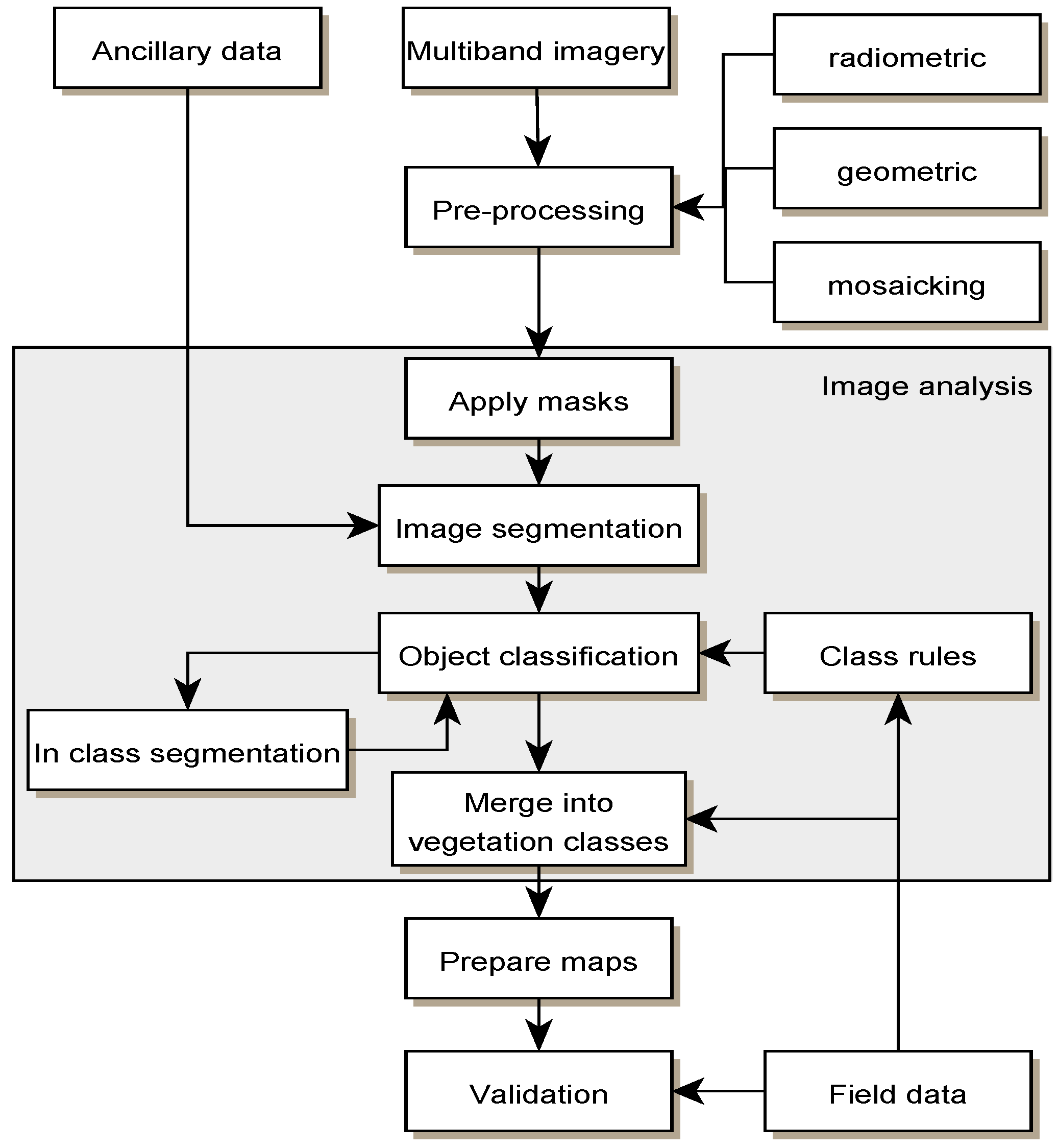
GEOBIA involves the partitioning of remotely sensed imagery into spectrally homogeneous image objects and using the spectral, spatial and topological features of the objects to assist with image classification. The classification of the image objects then not only uses the spectral features of the objects but also uses topological and hierarchical relationships between the image objects [18,21]. Ancillary data, such as topographic information, may also be included to improve classification accuracies. The steps of segmentation and classification are typically iterative through an analysis creating a step-wise approach to classification.
Coincident with the increasing use of GEOBIA applications for classifying HSR imagery has been the utilisation of sophisticated algorithms from machine learning, such as Random Forests (RF) as methods of interpreting HSR data [22]. RF is an ensemble classifier that builds a forest of classification trees, using a different bootstrapped training sample and randomly selected set of predictor variables for each tree. Unweighted voting is then used to produce an overall prediction for each site in the sample [22,23]. RF has been previously used for high accuracy vegetation classification in a number of mapping applications, including forest communities [24], invasive species [25,26,27], and the estimation the distribution of rare species [25]. It has also been shown to perform well in comparison to decision trees and other ensemble classifiers [28] and can capture complex, non-linear interactions among noisy, non-normal predictor variables [24,25]. In addition, RF provides measures of variable importance that can be used for further interpretation [24,25,28].
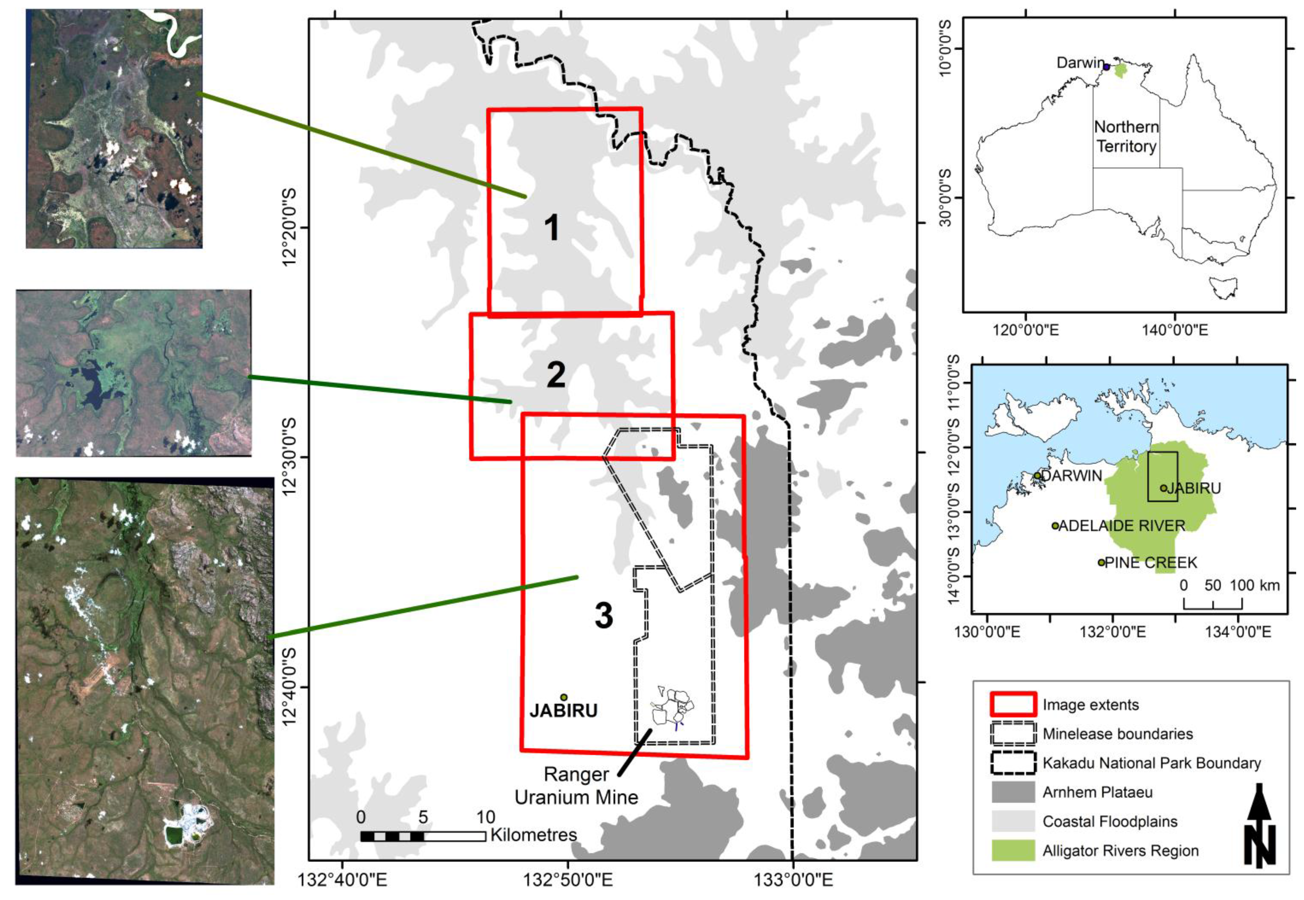
According to the criteria of the Ramsar Wetlands Convention, the wetlands within Kakadu National Park (KNP), Northern Australia have been designated as internationally important [29]. The wetlands, including the floodplain within the Magela Creek catchment are significant not only in their biogeographical context, but also for the diversity of plant communities [29] as well as habitat refuges for abundant and diverse waterbird populations [30,31]. KNP’s World Heritage listing in part refers to the natural heritage value of the diversity and endemism of the wetland vegetation [29]. Current landscape level ecological risks within the region are identified as weeds, feral animals and unmanaged wildfire [32]. In addition, the floodplain is a downstream receiving environment for Ranger Uranium Mine.
The spatial distribution of a number of the vegetation communities is annually dynamic, although reasons for the dynamics are not fully understood. The annual change has been observed as a naturally occurring phenomenon and, despite the importance of these wetlands, there has been little research of the dynamics [29]. Finlayson et al. [33] have postulated that the major determinant in the composition of flora was the duration and period of inundation, with lesser contributions from other factors such as water flow velocity and depth.
Mapping of the communities within the floodplain at the appropriate spatial and temporal scale can provide information to determine the drivers of the dynamics and establish a baseline for natural variability, which will be useful for monitoring this offsite environment when rehabilitation of Ranger uranium mine takes place. Vegetation community mapping of the floodplain will also inform ecological risk assessment that forms a basis for park management [32].
The aim of this project is to develop and test the utility of a decision-based methodology to accurately classify the vegetation communities of the Magela Creek floodplain using high spatial resolution multispectral satellite imagery and LiDAR-derived ancillary data. The procedure involves the application of GEOBIA techniques to segment and classify the imagery and data. To test the performance of the decision-based method, the results are compared against a Random Forests classification of the same data.

2. Methods

2.1. Study Site Description

The Magela Creek sub-catchment is located on the boundary between KNP and Western Arnhem Land, in the Alligator Rivers Region (ARR) of Australia’s Northern Territory about 250 km east of Darwin (Figure 1). The ARR covers an area of approximately 28,000 km2, including the World Heritage listed KNP. Magela creek is a seasonally-flowing tributary of the East Alligator River, originating in the sandstone Arnhem Land plateau [34]. There are ten distinct reaches of the creek [35]: The first seven reaches are channels intersecting the escarpment; the eighth reach consists of the anabranching sandbed channels of the lowlands (adjacent to Ranger Uranium Mine); the ninth reach is the narrow Mudginberri Corridor (a series of billabongs and connecting channels) and the Magela Creek floodplain (consisting mostly of seasonally inundated black-clay with a number of permanent billabongs); and the tenth is a single channel that flows into the East Alligator River. The corridor and floodplain sections (reach 9) are the focus of this research. The floodplain extent is over 220 km2.
Floodplain vegetation is primarily Paperbark (Melaleuca spp.) forests, open perennial and annual swamps, billabongs and grass/sedge/herb fields. Major ecological weeds are Para grass (Eurochloa mutica), and Salvinia molesta. Previous research has identified 10 major vegetation communities within the Magela Creek floodplain [33], the species composition of most communities can be seasonally dynamic [29]. The most recent community level vegetation map for the whole of the Magela Creek floodplain was based on time series (May–September 2006) Landsat 5 TM satellite imagery [9]. Sixteen classes were identified and then merged into 10 vegetation community types. This study has identified 12 vegetation classes. Hymenachne grassland is dominated by H. acutigluma throughout the year. Other species that may occur include Oryza meridionalis, Nymphaea spp., and Pseudoraphis spinescens [33]. The classes Melaleuca woodland and Melaleuca open forest typically contain M. cajaputi and M. viridiflora in the northern regions and at the edges of the floodplain, and M. leucadendra in the backswamps that are inundated for most of the year (December–August) [33]. Woodland communities have 10%–50% woody cover, whereas open forest communities have 50%–70% cover. These communities are typically inundated for 5–8 months of the year [29]. The Oryza grassland class is dominated by the annual grass, Oryza meridionalis towards the end of the Wet season. In the Dry, it is mostly bare ground or dead stems. The Pseudoraphis spinescens grassland class occurs in the southern half of the floodplain. The class, Pseudoraphis/Hymenachne consists of areas that are co-dominated by P. spinescens and H. acutigluma. Larger areas of Eleocharis dulcis sedgeland class mostly occupy the northern areas of the floodplain. The weed, Urochloa mutica (Para grass), is an invasive species from Africa that can form dense monocultures and outcompetes native vegetation in communities of Hymenachne, Oryza and Eleocharis [36]. This community occurs mostly in the central plains region. The class, Nelumbo herbland, is dominated by the water lilies, Nelumbo nucifera or to a lesser extent Nymphoides spp. These communities occur in permanent and semi-permanent wet areas. Other species that may be present include Leersia hexandra, Hymenachne acutigluma, Nymphaea spp. The floating fern, Salvinia molesta, can completely cover small areas of open water. The class, Leersia hexandra grassland can form large floating mats. The Mangrove communities are located mostly adjacent to the Magela Creek where it enters the tidal East Alligator River.
Figure 1. Location of the study site and extents of three WorldView-2 images used.
Remotesensing 07 11664 g001

2.2. Data Sets

The data sets used in this study included high spatial resolution multispectral satellite image, elevation and canopy height data and field data. The data sets are summarised in Table 1 and described in detail in the following sections.

2.2.1. Multispectral Data

The primary data set for this project consisted of three overlapping scenes of WorldView-2 (WV-2) multispectral data captured at approximately 1130 ACST, 11 May 2010. The sensors onboard the WV-2 satellite acquire data with image pixels representing 2 m ground sample distance (GSD) at nadir. The multispectral data consist of 8 spectral bands coastal (400–450 nm), blue (450–510 nm), green (510–580 nm), yellow (585–625 nm), red (630–690 nm), red edge (705–745 nm), NIR1 (770–895 nm), and NIR2 (860–1040 nm). For a detailed description of the sensor and data characteristics see Updike and Comp [37]. One feature that distinguishes WV-2 data from other HSR multispectral satellite data is the increased spectral resolution resulting from the inclusion of the coastal, yellow, red edge and NIR2 bands. Of particular interest to vegetation analysis is the red edge band which is optimal for the spectral characterisation of chlorophyll and water deficit in vegetation biomass, and thus useful for detecting vegetation under stress [38]. The red edge is defined as the abrupt change in leaf reflectance between 680 and 780 nm resulting from the strong chlorophyll absorption in the red and high reflectance in the NIR due to internal leaf scattering [39]. Red edge reflectance has been found to be strongly correlated to plant biochemical parameters (including chlorophyll content) and biophysical parameters (including leaf area index) [40]. Vegetation indices including the WV-2 red edge band have been used successfully to estimate wetland biomass [41].
Table 1. List of remotely sensed and field data used for the classification of Magela Creek floodplain vegetation communities, as well as the validation of the classification.
DataDateRelevant or Derived InformationUse of Data
WorldView-2 imageryMay 20108 spectral bands in VNIRSpectral class discrimination including derivation of indices
SRTM Digital Elevation ModelFebruary 2000Terrain (elevation)Floodplain boundary delineation
Air photo DEMJune 2006Terrain (elevation)Floodplain boundary delineation (upper reaches)
Canopy Height Model derived from LiDAR dataOctober 2011Canopy height and proportional cover of woody species (Melaleuca and mangroves)Identification of woody cover classes
Helicopter surveyMay 2010Dominant species and proportional coverValidation data
Airboat surveyMay 2010Proportional cover and species within homogeneous patchesValidation data
The imagery acquired covered approximately 730 km2 of the Magela Creek sub-catchment including the 220 km2 of the Magela Creek floodplain (Figure 1). As the requested study area exceeded the maximum swath width of the WorldView-2 satellite, three images were acquired during the satellite overpass (Table 2). The area of the image covered by Region 1 has approximately 1 km2 overlap with the Region 2 image. For Regions 2 and 3, there exists an overlap of 40 km2 between the two images.
The mean satellite azimuth for the Region 1 image was noticeably different to Regions 2 and 3 (Figure 2a). As a result, there was visible sun glint from patches of water in Region 1, where this is not evident in Regions 2 and 3 (Figure 2b).
Table 2. Summary of the specifications for the three WorldView-2 images acquired for this study.
Region 1Region 2Region 3
Time of capture11:15:19 CST11:14:28 CST11:14:41 CST
Scene centre12°19′26.28″S12°26′56.68″S12°32′21.55″S
132°50′7.23″E132°50′19.5″E132°53′6.92″E
Mean off-nadir view angle19.2°18.3°16.5°
Mean satellite azimuth237.2°323.2°311.2°
Mean satellite elevation68.4°69.3°71.3°
Area covered196 km2183 km2479 km2
Cloud cover0.0120.0090.014
Figure 2. (a) Azimuth (angle) and elevation (radial) of the satellite relative to the sun for each of the WV-2 image captures over Magela Creek floodplain, 11 May 2010. The position of the red circles represents the mean azimuth (angle) and elevation (radial) of the satellite for each of the images. The yellow circle represents the solar azimuth and elevation at the time of image capture. (b) The effect of different mean azimuth angles on the amount of sun glint from water on the floodplain for regions 1 and 2.
Remotesensing 07 11664 g002

2.2.2. Digital Elevation and Canopy Height Models

Terrain information in the form of two digital elevation models (DEMs) was included to aid in delineating the floodplain/uplands boundary and in masking out non-target land covers such as the surrounding savanna and escarpment outliers. This eliminated unnecessary analysis of non-floodplain surfaces. The primary DEM was Geoscience Australia’s 1 Arc Second Digital Elevation Model Version 1.0 derived from the Shuttle Radar Topography Mission (SRTM). The SRTM DEM with a spatial resolution of 30 m was included to enable the delineation of the floodplain boundary. A finer 10 m resolution DEM derived from a 2004 aerial photograph survey of KNP was also included for the purpose of delineating the upper reaches of the floodplain that were not well defined in the SRTM DEM.Initial analyses showed that the cover of Melaleuca spp. trees and shrubs and some grass and sedge cover, such as Eleocharis sp., were very similar spectrally and difficult to differentiate. A canopy height model (CHM) was incorporated into the project with the intent to distinguish between treed land cover and the spectrally similar but non-treed land cover. The CHM was derived from an airborne laser scanning (LiDAR) survey conducted within KNP between 22 October and 16 November 2011 using a Leica ALS60 laser scanner to collect the discrete multiple return data. The survey was undertaken by Fugro Spatial Solutions (FSS; www.fugrospatial.com.au). The LiDAR survey covered most of the floodplain apart from a couple of backwater swamps and some thin upper reaches. Based on 63 ground control points, the horizontal and vertical accuracy provided by FSS were 0.6 m and 0.2 m at 67% confidence levels, respectively. The root mean square error (RMSE) for the height was 0.090 according to FSS. The accuracy of the LiDAR data was independently checked by Geoscience Australia, who found the RMSE for the height was was 0.438 based on 14 GCPs provided by Northern Territory Government. The average point density was 2 m-2; the laser beam footprint was 0.32 m, and the flying height was 1400 m above ground level. The gridded digital surface model (DSM) and DEM were created through interpolation of the LiDAR point data. The DEM was derived from last returns which are assumed to have hit the ground. The DSM was derived from first returns which are assumed to hit the top of vegetation. The CHM was calculated by subtracting the bare earth model or DEM derived from the LiDAR data from the DSM. The CHM consisted of a grid of 2 m cells.

2.2.3. Field Data

Field data, solely for validation purposes and not used for training, were collected using two methods. Firstly, a ‘ground’ plot survey was undertaken 17–26 May 2010 using an airboat (a flat bottom boat driven forward by an aircraft-style propeller for shallow water operations). The survey provided 28 reference sites, each representing homogenous cover consisting of one species. The sampling method used for this survey was random (although confined by accessibility) with the reference data collected using an oblique visual estimation of the projected cover by species. These observations were made from the deck of the airboat while stationary. The second method involved a systematic helicopter survey undertaken on 29 May 2010. This survey provided a further 100 reference sites. For these sites, the location, dominant species and proportional cover were recorded based on visual estimates from photos taken during the flight. All 128 sites are shown in Figure 3, although two were not used; one due to aligning with cloud cover and the other was outside the area of study.

2.3. Image Pre-processing and Analysis

The steps involved pre-processing and analysing the data are shown in Figure 4. Analysis was based on the geographical object-based image analysis (GEOBIA) approach.
All imagery were geometrically orthorectified using the sensor’s rational polynomial coefficients and ground control points (GCPs) based on easily identifiable tarpaulins placed throughout the scene with centre point locations recorded using a differential GPS. The surface model for the orthorectification was the SRTM DEM data set. Accuracy assessment of the rectification was based on six independent GCPs with a root mean square error of 1.82 m [42,43].
Figure 3. Location of reference data collected across the floodplain.
Remotesensing 07 11664 g003
The three images were then radiometrically calibrated to surface reflectance using the FLAASH atmospheric correction algorithm based on the MODTRAN radiative transfer model [44]. Two validation methods were used to determine the quality of FLAASH surface reflectance model. The first method involved comparing sample areas of the FLAASH corrected imagery with the corresponding field-based reflectance. Within the Regions 2 and 3 imagery, mean FLAASH reflectance values for each band were extracted for locations corresponding to a total of 24 targets measured in the field along with two calibration panels. Field spectra were collected between the hours of 10:00 a.m. and 3:00 p.m. local time using a FieldSpecPro-FR spectrometer (covering 350–2500 nm) (ASD Inc). Spectra were captured using a 25º field of view (FoV) at nadir with the averaging sample spectrum set to 25. The sensor height was set to 1 m for targets on land and 0.5 m over water, resulting in an approximate ground view swath of 44 cm and 22 cm in diameter, respectively. A Labsphere Spectralon® white reference panel was used for calibration. Between each white reference sample and dark current calibration, a maximum of four spectral samples were collected. The number of samples (between 9 and 25) obtained for each target was dependent on the variance observed within the target. The area sub-sampled for most targets was 25 m2. The location of each target was recorded using a GPS. The Region 1 image was not considered in this validation as no field spectra were collected for this region. A block of at least six pixels were extracted for each target from the FLAASH corrected imagery avoiding mixed pixels and adjacency effects.
Figure 4. The image analysis approach used for wetland vegetation mapping.
Remotesensing 07 11664 g004
The second validation method compared reflectance from the FLAASH model with previously published empirical line (EL) modeled reflectance derived from the same imagery [43]. Two hundred randomly sampled points were generated within both Region 2 and 3. The corresponding pixel values for each band for both EL- and FLAASH- derived reflectance data sets were assigned to each of the random points. The EL- and FLAASH- derived reflectance values were then plotted against the other and r2 values determined. Again, the Region 1 image was not able to be validated due to no ground-based spectra available.

2.4. Image Segmentation

The image was segmented in a number of steps. The first segmentation was used to delineate the floodplain boundary to confine further analysis to the floodplain. There is a visibly distinct boundary between most of the floodplain and the surrounding savanna in the WV-2 imagery and a contour based on the SRTM DEM at 6 m closely approximated this boundary. Thus, a threshold height (z) value of 6 m based on the SRTM DEM was used to split the imagery into floodplain (z < 6 m) and non-floodplain (z ≥ 6 m) objects for the majority of the floodplain. However, the lack of spatial detail in the SRTM DEM (30 m GSD) was less effective in delineating the boundary in the upper reaches of the floodplain (towards the southern extent of the imagery) and the boundary was poorly defined. To compensate for this, the finer scale aerial photography based DEM (10 m GSD) was used for boundary delineation for the upper reaches with the same height threshold value. The boundary was then manually adjusted within a GIS using visual interpretation of the WV-2 imagery to provide a complete floodplain boundary. Further processing and analysis was restricted to within the floodplain object.
After floodplain delineation, the imagery within the floodplain boundary was split into two segments based upon the view angles shown in Figure 2: (a) a Region 1 object and (b) a Regions 2 and 3 object. Subsequent image processing and analysis was varied for each of these two segments due to the view-angle-based spectral differences. However, both objects were further segmented into image objects using the multiresolution segmentation algorithm within the eCognition® image processing software [21]. The algorithm is based upon the fractal net evolution approach [45] and is primarily an iterative bottom-up segmentation method starting with individual pixels and merging these pixels based upon pixel heterogeneity and object shape and colour [46]. These are determined within the algorithm by two parameters; (i) scale and (ii) colour versus form. The scale parameter within the algorithm is set by the operator and is influenced by the heterogeneity of the pixels. The colour parameter balances the homogeneity of an object’s colour with the homogeneity of its shape. The form parameter (compactness) is a balance between the smoothness of a segment’s border and its compactness. The weighting of these parameters establishes the homogeneity criterion for the image objects. Visual inspections of the image objects resulting from a number of segmentations using variations in parameter weightings were used to determine the overall optimal weighting which were scale parameter = 200, colour = 0.7 and compactness = 0.3.

2.5. Analysis

Analysis of the image objects involved two main steps: (1) separating treed and non-treed cover classes based on the CHM; and (2) implementing a decision tree classification on the non-treed objects based mainly on the spectral information of the image objects.

2.5.1. Separating Woody from Non-Woody Cover

The LiDAR derived CHM was used to distinguish image objects that contained trees from image objects with no trees (Figure 5). A detailed description of this method can be found in [47]. The method involved identifying potential candidate objects containing trees using a minimum mean canopy height threshold of 0.8 m. Objects with mean canopy heights above this threshold were assumed to have high above ground biomass, which may include trees and were assigned as potentially treed objects. Within the potentially treed objects, sub-objects representing trees or clusters of trees were created using a threshold segmentation algorithm assuming trees consisted of cells of the CHM above 4 m (the observed minimum height of detectable trees). Sub-objects with spurious high values were removed from the treed objects class using 25 m as a ceiling value. Additionally, objects were eliminated from the potentially treed class if they contained no tree sub-objects. The remaining treed objects were then assigned to a tree class depending on the proportion of tree sub-objects per treed object: Open forest was greater than 50% proportional cover, Woodland 10%–50% proportional cover, Open Woodland less than 10% proportional cover. To maintain cover proportions consistent with those described in the Australian Soil and Land Survey Field Handbook [48], the Open woodland and Woodland were grouped together into a single Woodland class. In Region 1, treed objects were assigned to the Mangrove class based on proximity to the East Alligator River. Otherwise they were assigned as either Melaleuca open forest or Melaleuca woodland. In Regions 2 and 3, there were no Mangroves, so objects were assigned as either Melaleuca open forest or Melaleuca woodland. For floodplain objects outside the LiDAR coverage (two backswamp reaches), classification was conducted as for non-treed objects.
Figure 5. A potentially treed object (red polygon) (a) the Canopy Height Model (b) and tree sub-objects (c) Scale bar on top left of each image is 100 m.
Remotesensing 07 11664 g005

2.5.2. Manual Decision Tree Classification

The classification of the non-treed image objects into the vegetation community classes was implemented using a set of rules that followed a decision tree classification model. Decision tree (DT) analysis uses the dichotomous splitting of data based on thresholds of the most relevant variables in the data. The advantages of using a decision tree classification over standard statistical classifiers are that they can (i) incorporate a variety of data sources (such as the multispectral imagery, digital elevation models and canopy height models used here); (ii) handle both continuous and categorical information; and (iii) the most important variables among those available for the classification are selected [49].
The DT analysis used progressive dichotomous grouping of the non-treed image objects using thresholds that formed the basis of the splitting rules. The thresholds incorporated into the rules were predominantly based upon the four spectral indices described in Table 3. Based upon observed surface spectral variations between the image objects and analysis of the mean feature values and statistics of objects of known vegetation types, the thresholds decided upon were considered optimal for splitting groups of objects. The four spectral indices (Equations (1)–(4)) used were: (i) the forest discrimination index (FDI) after Bunting and Lucas [50]; (ii) the NDVI or Normalized Difference Vegetation Index [51]; (iii) the Enhanced Vegetation Index (EVI) [52]; and (iv) a band ratio, (NREB) was also included that appeared useful in discriminating Nelumbo spp. cover. Within the imagery, the greatest reflectance difference and visual contrast between the floating or emergent broad-leafed vegetation and other vegetation (including grasses) was observed in the three-dimensional feature space described by the NIR2, Red edge and Blue bands (Figure 6). Based on this, an assumption was made that a reliable separation between the two cover types could be achieved via a combination of the three bands. The premise of the NREB is that, for the time of year of image capture, the broad-leafed macrophytic vegetation (typically broad horizontal leaves) displays greater homogeneity in cover than the grasses (typically a mixture of thin green leaves, vertical stems and shadowing) producing a higher NREB value (Figure 7). Additionally, the band ratio has been shown to successfully map Nelumbo spp. cover from multitemporal WV-2 imagery over the area [47].
Figure 6. Three dimensional plot of feature space for the NIR2, Red edge and Blue bands. This shows the separation between sample objects of Nelumbo sp. and other vegetation types.
Remotesensing 07 11664 g006
The decision trees for Region 1 and Regions 2 and 3 are shown in Figure 8 and Figure 9 respectively. For some branches of the decision trees, it was necessary to undertake further segmentation to split some objects into smaller objects (using scale parameters of 100 and 50) to achieve further class discrimination.

2.5.3 Random Forests Classification

The classification of the non-treed image objects into the vegetation community classes was also implemented using the Random Forests ensemble classifier. In the RF analysis, the number of samples was 135. The samples used were selected using a systematic sampling method to ensure a minimum of 6 samples per class and identified using expert visual analysis of a pan-sharpened version (GSD 0.6 m) of the imagery. For the other parameters, the number of trees was set to 200 and the number of features used was eight. These were the four indices from Table 3 plus four band values: mean Green, mean Red Edge, Standard deviation NIR 2, and Standard deviation Red Edge, as per the DT method. Additionally, in line with the DT method, separate RF classifications were run for Region 1 and Regions 2 and 3. For each of the two regions, separate RF classifications were conducted also for areas within and outside the coverage of the CHM.
Figure 7. Object values for the band ratio NIR2+RE−B for a sample of objects of Nelumbo spp. and other floodplain vegetation. Dashed horizontal line is the mean for the Nelumbo spp. objects in the graph and the solid line is the mean for the Other objects.
Remotesensing 07 11664 g007
Figure 8. The decision tree for the classification of Region 1 objects.
Remotesensing 07 11664 g008

2.6. Accuracy Assessment

The accuracies of the classified floodplain vegetation maps for 2010 were assessed by comparing the vegetation community described in the map to the community defined in the reference (field) data at those particular locations. These comparisons were undertaken using confusion matrices [53] From the matrices, User’s and Producer’s accuracies were calculated for each class along with the overall classification accuracies, and the Kappa statistics [54]. While Kappa indices have long been popular in remote sensing literature as a measure of overall accuracy [53], their worth has recently been criticised as (a) they provide no extra information that is not already provided by the overall accuracy; (b) are hard to interpret and (c) can be misleading [55]. Kappa is included here purely for comparison to other studies.
Figure 9. The decision tree for objects in Regions 2 and 3.
Remotesensing 07 11664 g009
To provide further information on the accuracy of the classification, the confusion matrices for each classification were summarized by computing quantity disagreement and allocation disagreement [55]. Quantity disagreement is the difference between the reference and the classification categories due to an imperfect match in the overall proportions of all mapped categories. Allocation disagreement is the difference between the reference and the classification due to an imperfect match in the spatial allocations of the mapped categories, given the categorical proportions in the reference and classification. The allocation disagreement was split into two components: exchange and shift [56]. Exchange is the component of allocation disagreement that pairwise confusions cause and shift is the component of allocation disagreement that non-pairwise confusions cause [56]. The total disagreement or error is the sum of the quantity disagreement, exchange and shift.
Table 3. The spectral indices used in the decision tree classifications. FDI = forest discrimantaion index, NDVI = normalized difference vegetation index, EVI = enhanced vegetation index and NREB is a band ratio. Blue = blue band, NIR2 = near infrared 2 band, Red = red band, RE = red edge band.
IndexEquationIndex Notes
FDI N I R 2 ( R E + B l u e ) (1)Enabled the separation of photosynthetic vegetation from bare soil and non-PS vegetation. In particular, it separates woody canopy from understorey and ground cover.
NDVI N I R 2 R e d NIR2+Red (2)Strongly related to photosynthetic material. Enabled discrimination between actively photosynthesising vegetation, senescent vetation such as Oryza, and open water.
EVI* G × ( N I R 2 R e d ) ( N I R 2 + ( C 1 × R e d ) + ( C 2 × B l u e ) + L (3)Songly correlated to evapotranspiration.
NREB ( N I R 2 + R E ) B l u e (4)Highlighted photosynthetic vegetation that is highly reflective and homogeneous; in this case, emergent communities dominated by Nelumbo, Leersia, and Salvinia.
* G=2.5, C1=6, C2=7.5 and L=1.
Two tests were conducted to compare the results of the DT and RF classifications, assuming the null hypothesis that the same population proportion of objects was correctly classified for both classification methods. A z-test was conducted using the Kappa value from both classifications [53]. In addition, a McNemar’s test [57,58] was used to test the significance of the difference between the decision tree (DT) and the RF classifications. The test is based on the chi-squared statisitic (χ2) and is calculated using Equation (5):
χ 2 = ( f 12 f 21 ) 2 ( f 12 + f 21 )
where f12 was the number of correct samples for the first classification that were incorrect in the second, and f21 was the number of correct samples for the second classification that were wrong in the first.

3. Results

3.1. Accuracy of the FLAASH Radiometric Calibration

In the comparison between the field spectra and FLAASH derived reflectance (Figure 10), all bands showed statistically significant relationships between FLAASH derived reflectance and field reflectance data. r2 values for bands 1 to 6 were greater than 0.9. Bands 7 and 8 (the NIR bands) recorded slightly lower r2 values (0.85 and 0.82 respectively), primarily due to the influence of two outliers over water. In the regression analysis between all bands in the FLAASH derived reflectance and the EL reflectance from [43], r2 was greater than 0.99.

3.2. Classification Accuracy

From the confusion matrix for the DT classification, the overall accuracy was 78% with a Kappa value of 0.75. User’s and Producer’s accuracies for each class are shown in Table 4. The most accurately delineated classes were Leersia, Melaleuca woodland and Para Grass with Producer’s accuracies of 80.1%, 90%, and 87.5%, and User’s accuracies of 100%, 90% and 87.5%, respectively. The Mangrove and Melaleuca open forest classes also had high accuracies (Producer’s accuracies of 100% and User’s accuracies of 75%) however, the total number of reference samples for each of these classes was quite low (three each). A low Producer’s accuracy (57.9%) indicates there was confusion where Eleocharis was misclassified as Hymenachne (four instances), Oryza (two instances), Mangroves or Melaleuca woodland (both one instance). Of those classes with low User’s accuracies, 24 sites that were classed as Hymenachne, nine were other classes according to the reference data with four being Eleocharis. In addition, there was some confusion between the Pseudoraphis/Hymenachne class and the separate Pseudoraphis and Hymenachne classes. After merging these three classes, the overall accuracy of the classification increased to almost 84%.
The overall error for the DT classification of the Magela Creek floodplain was 22%. Quantity disagreement accounted for half of the total error, while exchange (8%) was greater than shift (3%) in the allocation disagreement. Figure 11a summarises the categorical errors for each of the 13 categories of the DT classification. The three classes that contributed least to the error were Melaleuca Open Forest, Mangrove and Leersia (0.8% quantity disagreement each). Hymenachne was the class contributing the most error (9.5%) divided equally between quantity disagreement and exchange. Most of the error was commission meaning the extent of Hymenachne was over estimated. The class with the next highest proportional error is Eleocharis with just over 7%, which was mostly quantity disagreement showing the class was under estimated in the classification.
From the confusion matrix for the RF classification (Table 5), the overall accuracy was 66.7% with a Kappa value of 0.6. The most accurately delineated class was Melaleuca open forest with Producer’s accuracy of 100% and User’s accuracy of 75%. The Melaleuca woodland and Oryza classes also had high Producer’s accuracies (100% and 85.7%, respectively) however the User’s accuracies were low (66.7% and 60%). The low Producer’s accuracy (33.3%) indicates there was confusion where Mangroves was misclassified as other woody classes. As for the DT classification there was some confusion between the Pseudoraphis/Hymenachne class and the separate Pseudoraphis and Hymenachne classes resulting in low Producer’s and User‘s accuracies for these classes. By merging these three classes, the overall accuracy of the classification increases to 74%.
Figure 10. Regression plots comparing the FLAASH modelled surface reflectance with field based (ASD) reflectance measurements of all targets (including calibration tarpaulins) for all 8 WV-2 bands.
Remotesensing 07 11664 g010
Table 4. Accuracy matrix for the decision tree classification.
Reference Data
EleocharisHymenachneLeersiaMangroveMelaleuca Open ForestMelaleuca WoodlandNelumboOryzaPara GrassPseudoraphis/HymenachnePseudoraphisSalviniaOpen WaterTotalCommissionUA (%)
Classified dataEleocharis1110000000000012191.7
Hymenachne4150001011101024962.5
Leersia004000000000040100
Mangrove10030000000004175
Melaleuca Open Foreest00003000000014175
Melaleuca Woodland1000090000000101090
Nelumbo00100050000017271.4
Oryza20000006000008275
Para Grass01000000700008187.5
Pseudoraphis/ Hymenachne0100000001322018572.2
Pseudoraphis00000000025018362.5
Salvinia000000000008210280
Open Water000000000000990100
Total1918533105781671114126
Omission8310010113235
PA (%)57.983.3801001009010085.787.581.371.472.764.3
Overall Accuracy (%)77.8%
Table 5. Accuracy matrix for the Random Forests classification.
Reference Data
EleocharisHymenachneLeersiaMangroveMelaleuca Open ForestMelaleuca WoodlandNelumboOryzaParaGrassPseudoraphis/HymenachnePseudoraphisSalviniaOpen aterTotalCommissionUA(%)
Classified dataEleocharis1210000000000013192.3
Hymenachne41010000013102221245.5
Leersia003000000000030100
Mangrove000100000000010100
Melaleuca Open Forest00013000000004175
Melaleuca Woodland1101010100100015566.7
Nelumbo00000030000227442.9
Oryza110000061001010460
Para Grass121000016100012650
Pseudoraphis/Hymenachne010000000810010280
Pseudoraphis020000000350010550
Salvinia000000000007070100
Open Water0000001000011012283.3
Total1918533105781671114126
Omission7822002128244
PA (%)63.255.66033.310010060.085.7755071.463.671.4
Overall Accuracy (%)66.7%
Figure 11. Categorical errors for each of the 13 classes for the Magela Creek floodplain for (a) DT classification and (b) RF classification.
Remotesensing 07 11664 g011
The overall error for the RF classification of the Magela Creek floodplain was 33%. Quantity disagreement accounted for over half of the total error (17%), while exchange (11%) was greater than shift (5%) in the allocation disagreement. Figure 11b summarises the categorical errors for each of the 13 categories of the RF classification. The three classes contributing least to the error were Melaleuca Open Forest, Mangrove and Leersia (0.8% quantity disagreement each). Hymenachne was the class with the most error (16%) divided between quantity disagreement (3%), shift (6%) and exchange (6%). This means that while some of the Hymenachne class was over estimated in extent, most of the error was actually confusion with other classes. The class with the next highest proportional error is Pseudorpahis/Hymenachne with 8%, which was mostly quantity disagreement showing the class was under estimated.

3.3. Image Classification

The resultant maps from the DT classification (Figure 12) and the RF classification (Figure 13) both consisted of 12 vegetation classes consistent with classes previously described in the literature as being present on the floodplain [33]. Also included is open water. Table 6 shows the area for each class from both classifications. The extent of the Leersia, Oryza, Para grass, Pseudoraphis/Hymenachne Open water classes was noticeably greater in the DT classification, while the extent of the Hymenachne, Melaleuca woodland and Pseudoraphis classes were greater in the RF classification. The RF classification mapped half the extent of the Mangrove communities compared to the DT classification (123 ha to 249 ha).
From Table 7, it can be seen that the two features within the RF classification with the highest importance were the NREB band ration and the Mean Red edge.
Table 6. Areas for each class for both classification methods.
Decision TreeRandom Forests
Class nameArea (ha)Area (ha)
Eleocharis10541291
Hymenachne36395116
Leersia96769
Mangrove249123
Melaleuca open forest8221020
Melaleuca woodland50395917
Nelumbo243267
Oryza40401820
Para grass21811095
Pseudoraphis/Hymenachne375143
Pseudoraphis9431441
Salvinia108225
Open Water35892400
Table 7. Importance (proportional) of features used in the RF classification.
FeatureRegion 1Region 23Region 1 outside CHMRegion 23 outside CHM
Mean Green0.100.080.090.09
Mean Red edge0.170.180.170.18
Standard deviation NIR20.110.100.110.11
Standard deviation Red edge0.120.120.130.13
EVI0.120.110.120.11
FDI20.100.100.100.10
NDVI20.110.120.120.12
NREB0.170.190.160.16
Figure 12. Vegetation map for the Magela Creek floodplain based on DT classification, 11 May 2010.
Remotesensing 07 11664 g012
Figure 13. Vegetation map for the Magela Creek floodplain based on RF classification, 11 May 2010.
Remotesensing 07 11664 g013
The z-value between the Kappa values for the two classifications was 2.42, which is greater than the critical value for z at the 98% confidence level (2.33). The McNemar’s test statistic was 9.8 which is significant at p-value of 0.01. Therefore, based on the results of these two tests, the null hypothesis of equal classifier performance is rejected. The DT classifier produced more accurate results than the RF classifier.

4. Discussion

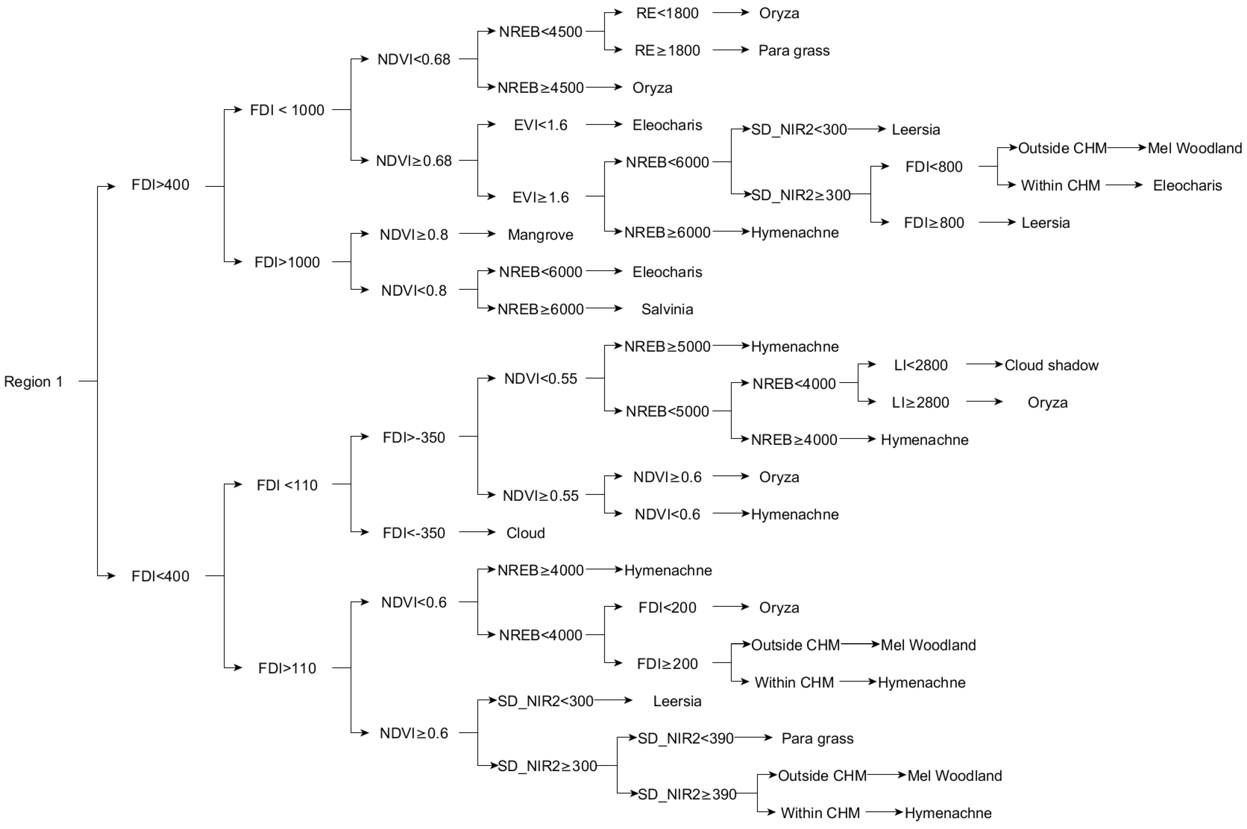
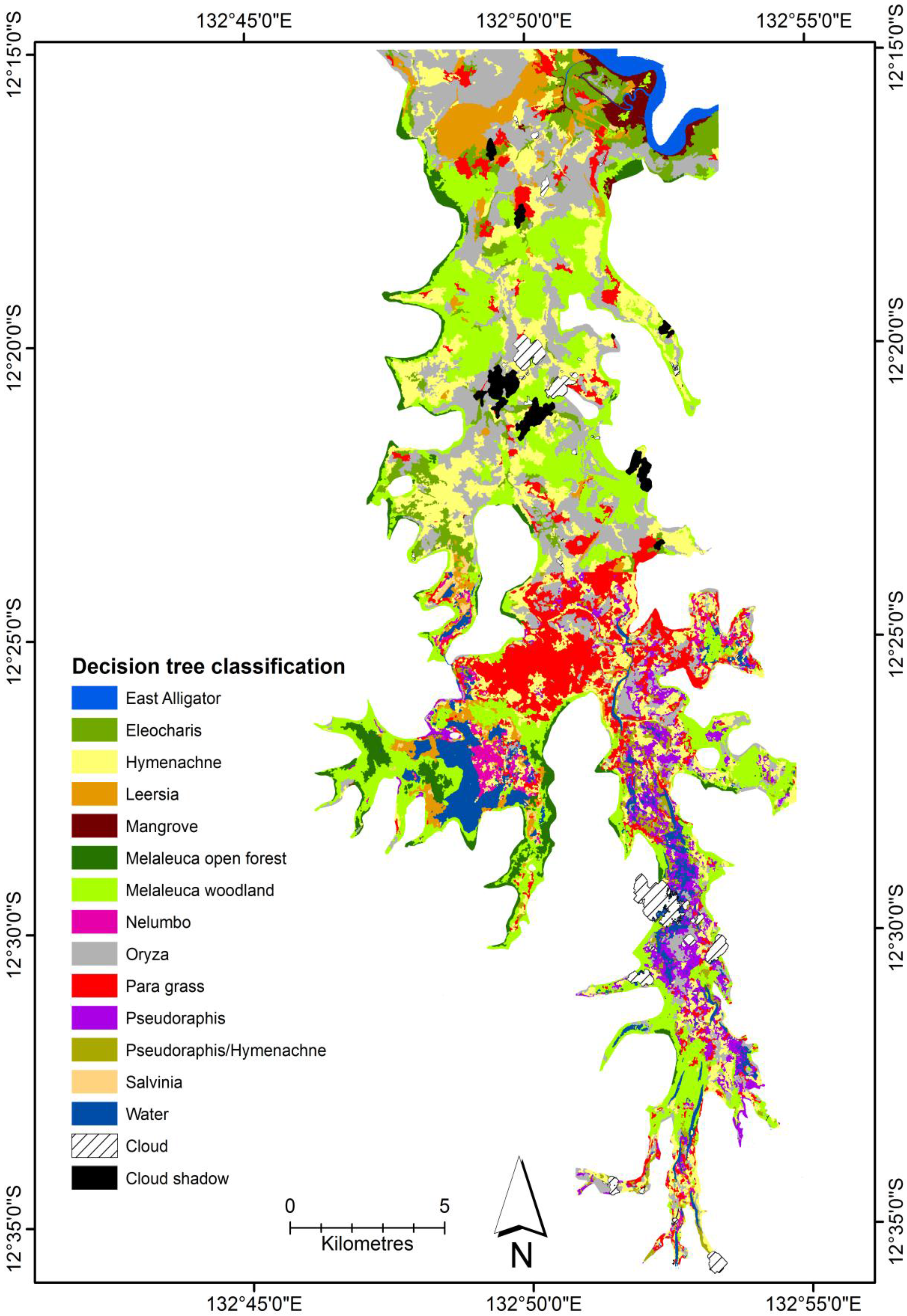
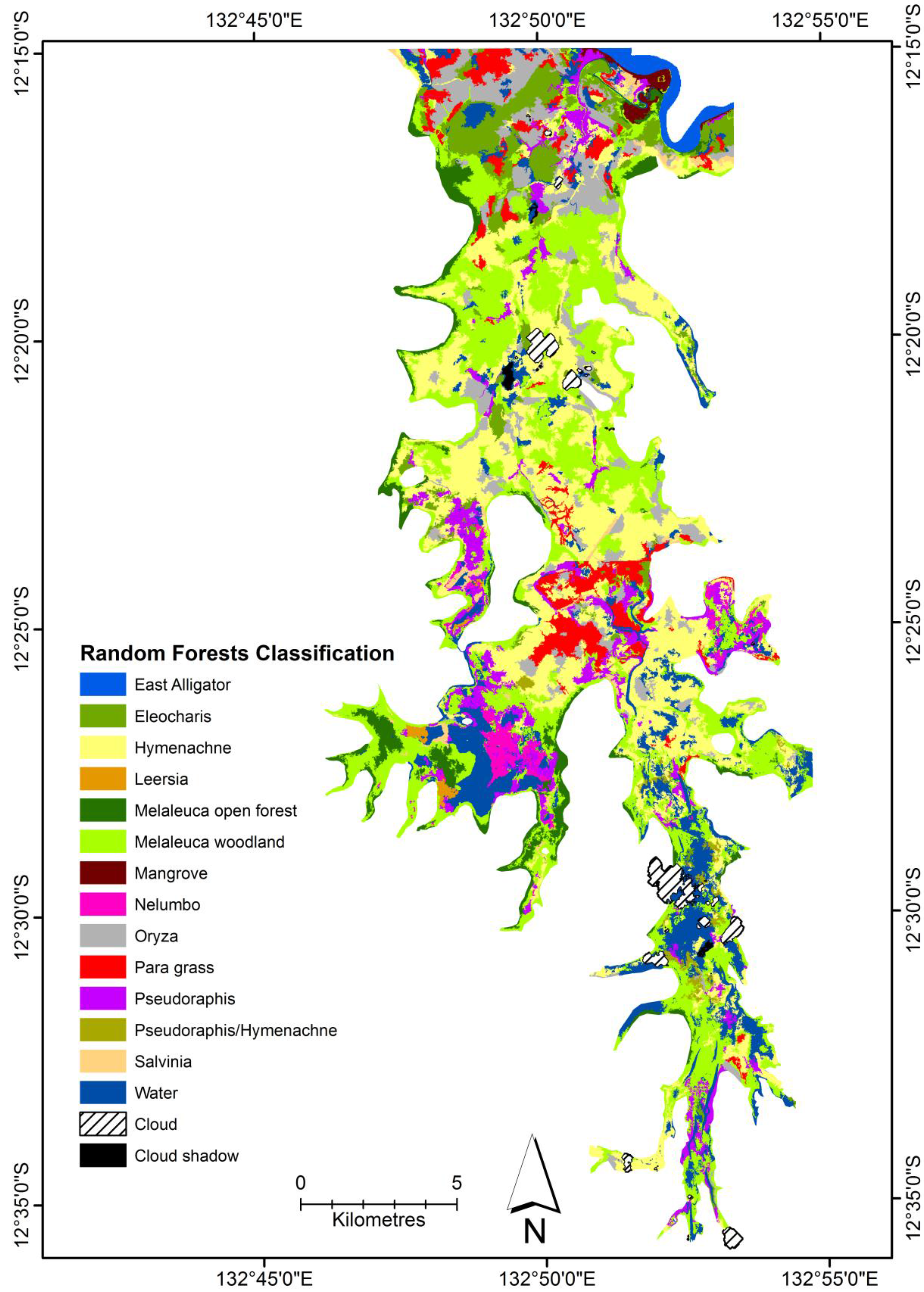
For this study, a decision tree classification was developed for classifying WorldView-2 imagery to map the vegetation on the Magela Creek floodplain. In addition, the results were compared to a RF classification of the same data. Overall, the DT classification clearly outperformed the RF classification as shown in the statistical tests undertaken. In addition, most classes were more accurately classified in the DT classification. This is most likely because the RF classification was reliant on purely on the statistical information from the samples selected, whereas in the DT classification the operator was able to select what feature to use and specify the threshold value to apply. Therefore, a manually derived decision tree does have merit especially where there are classes that are difficult to map based on purely using statistical methods. The performance of the rule set over the state of the art supervised classification method, Random Forests, suggests that the DT method may be a useful alternative for areas where wetland maps created using a supervised classification have less than satisfactory accuracies. The method is temporally transferrable, having been used to map vegetation on the Magela Creek floodplain for subsequent years 2011–2013 with only minor adjustments to thresholds to account for spectral variation due to slight differences in view angle and seasonality [47]. One way to test whether the method is spatially transferrable would be to apply it other wetlands in the region, which are quite different in composition [29].
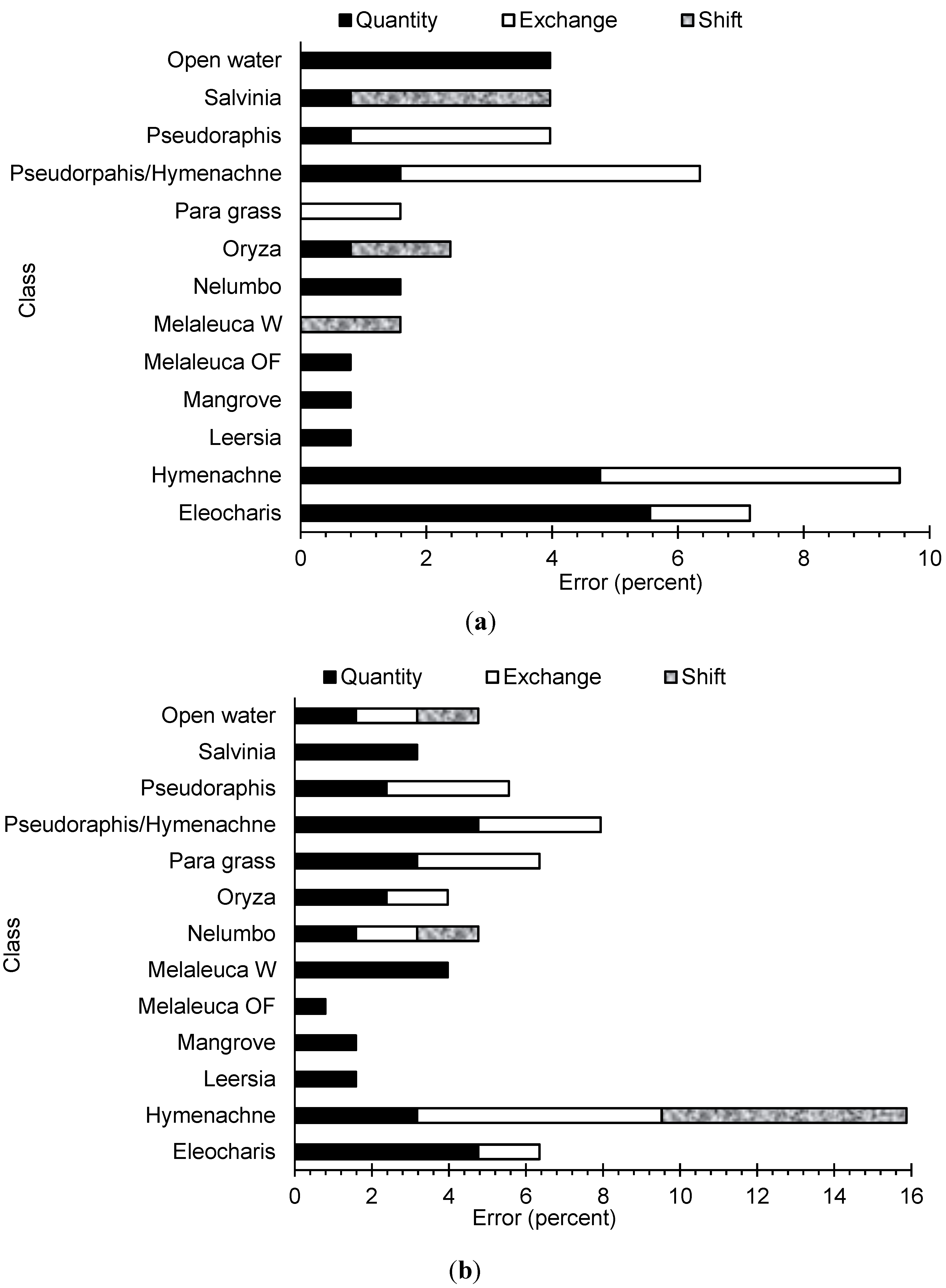
Both vegetation classification processes were able to distinguish between the spectrally and structurally distinct vegetation communities within the floodplain. The use of multiple indices and ratios were able to differentiate between classes that appeared spectrally similar. From the summaries of the confusion matrix, there were a number of instances where objects were either not detected or misclassified. There was some difficulty in distinguishing between vegetation classes that are spectrally similar, most notably between the classes dominated by grasses. Previously, there has been noted some spectral similarity between different covers namely Oryza and Para grass [36]. Most of the uncertainty in the maps is due to the confusion between grass classes. By merging the three grass classes (Pseudopraphis, Pseudoraphis/Hymenachne and 
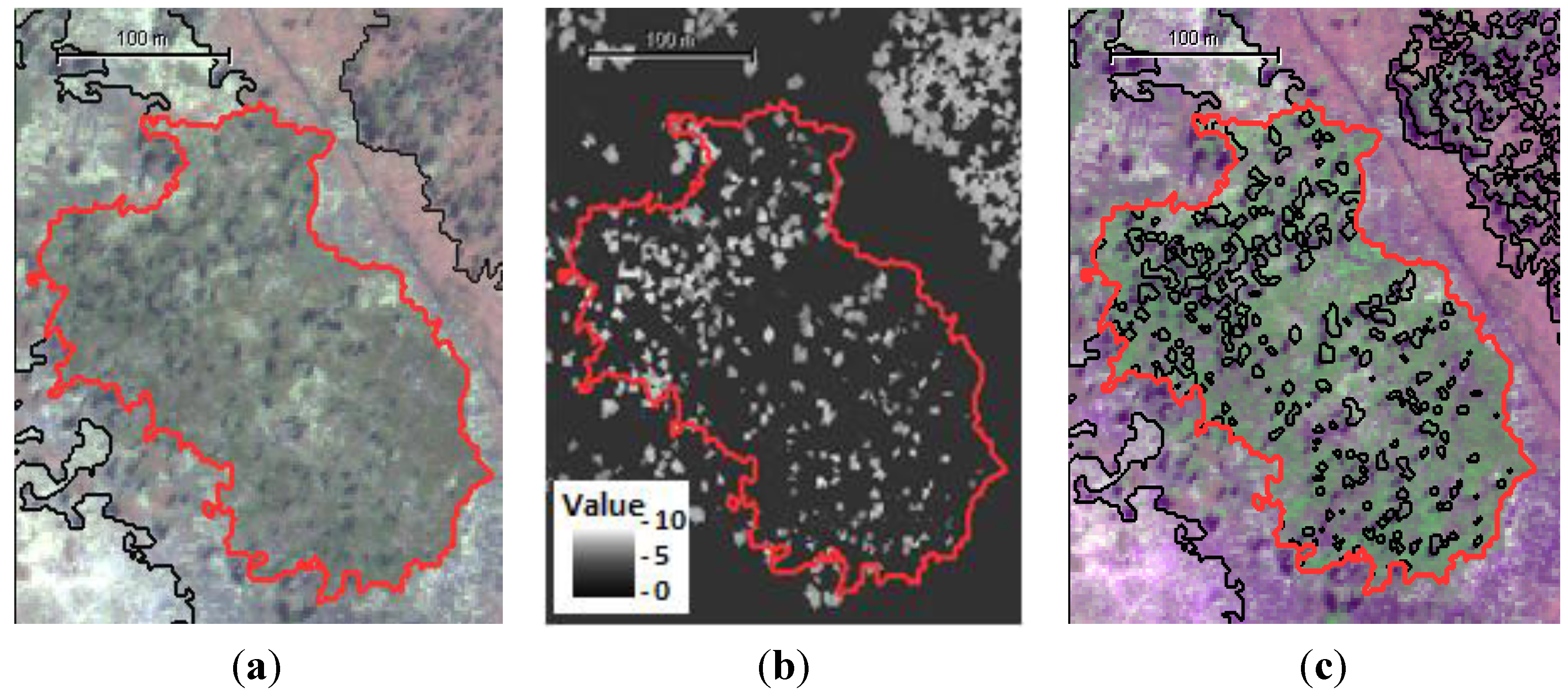
Hymenachne), the overall accuracies were for both classifications were increased by over 7%. In addition, there were objects that were of the same class of vegetation cover that were spectrally different. This is more than likely due to differences in growth phases as a result of water availability. For example, the floodplain margin will dry out quicker and grasses senesce or die earlier than those in the central floodplain. In addition, the inclusion and analysis of the CHM was successfully able to differentiate between spectrally similar but structurally different communities. Initial analysis, not presented here, based on the decision tree without the CHM saw overall accuracies 10% less, due to confusion particularly between trees and patches of Eleocharis.
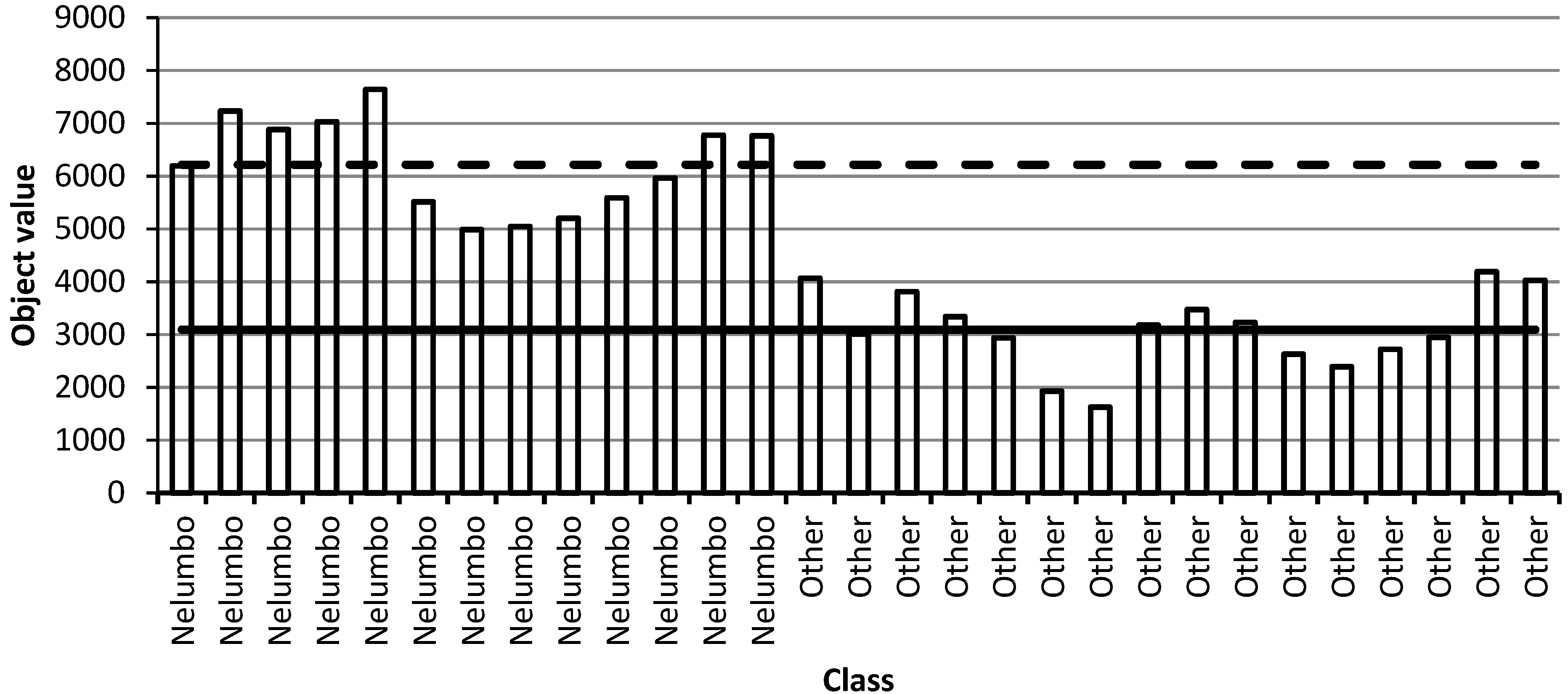
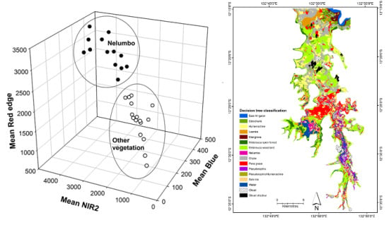
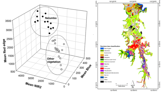
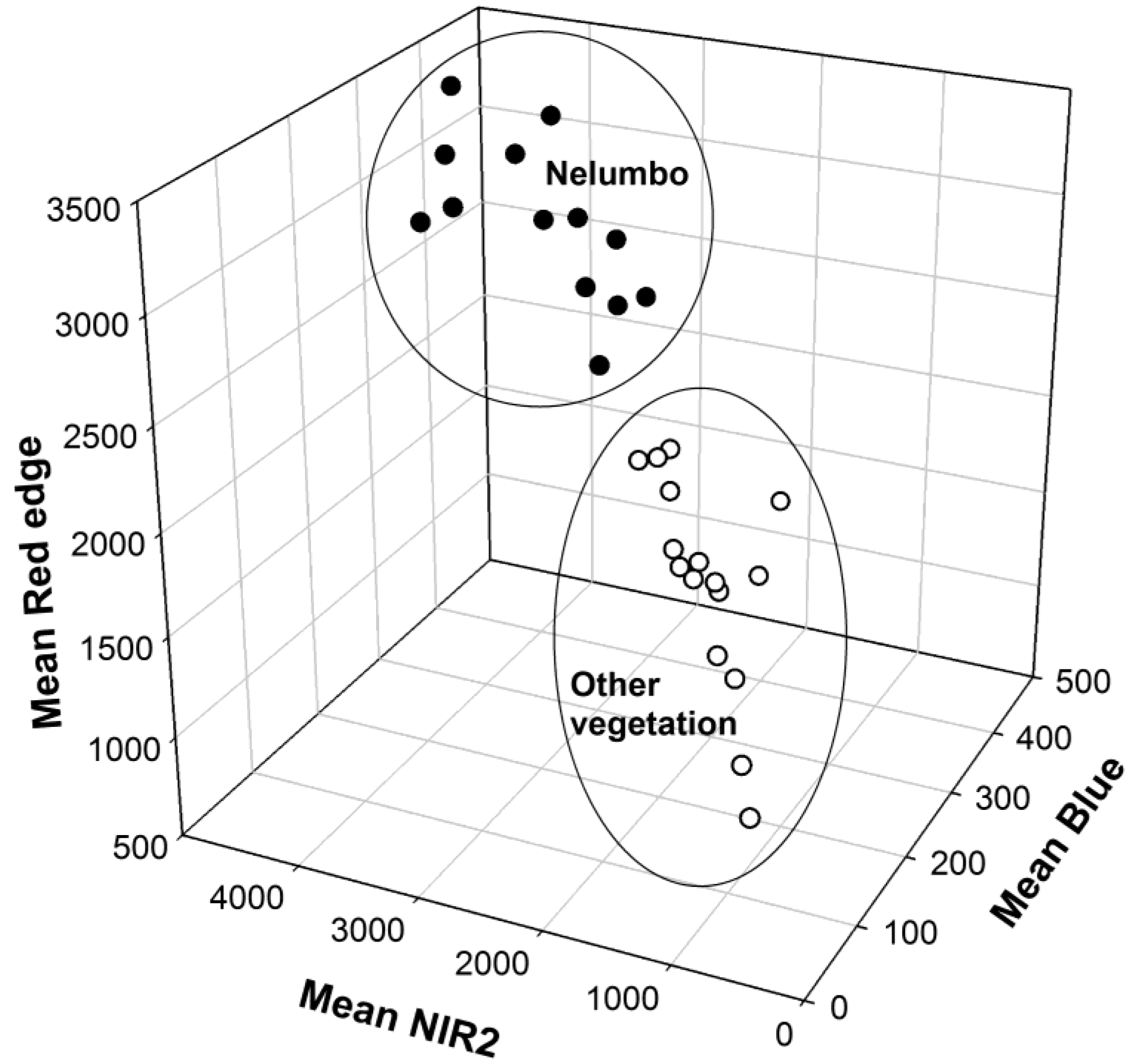
One outcome of interest from this research is the potential utility of the band ratio, NREB, for the classification of stands of emergent vegetation with floating leaves such as lilies. The use of the NREB ratio has been successful for mapping these stands on the floodplain over multiple dates using WV-2 imagery [47]. Further testing of this ratio could be conducted to assess its potential in this regard for wetlands in other regions.
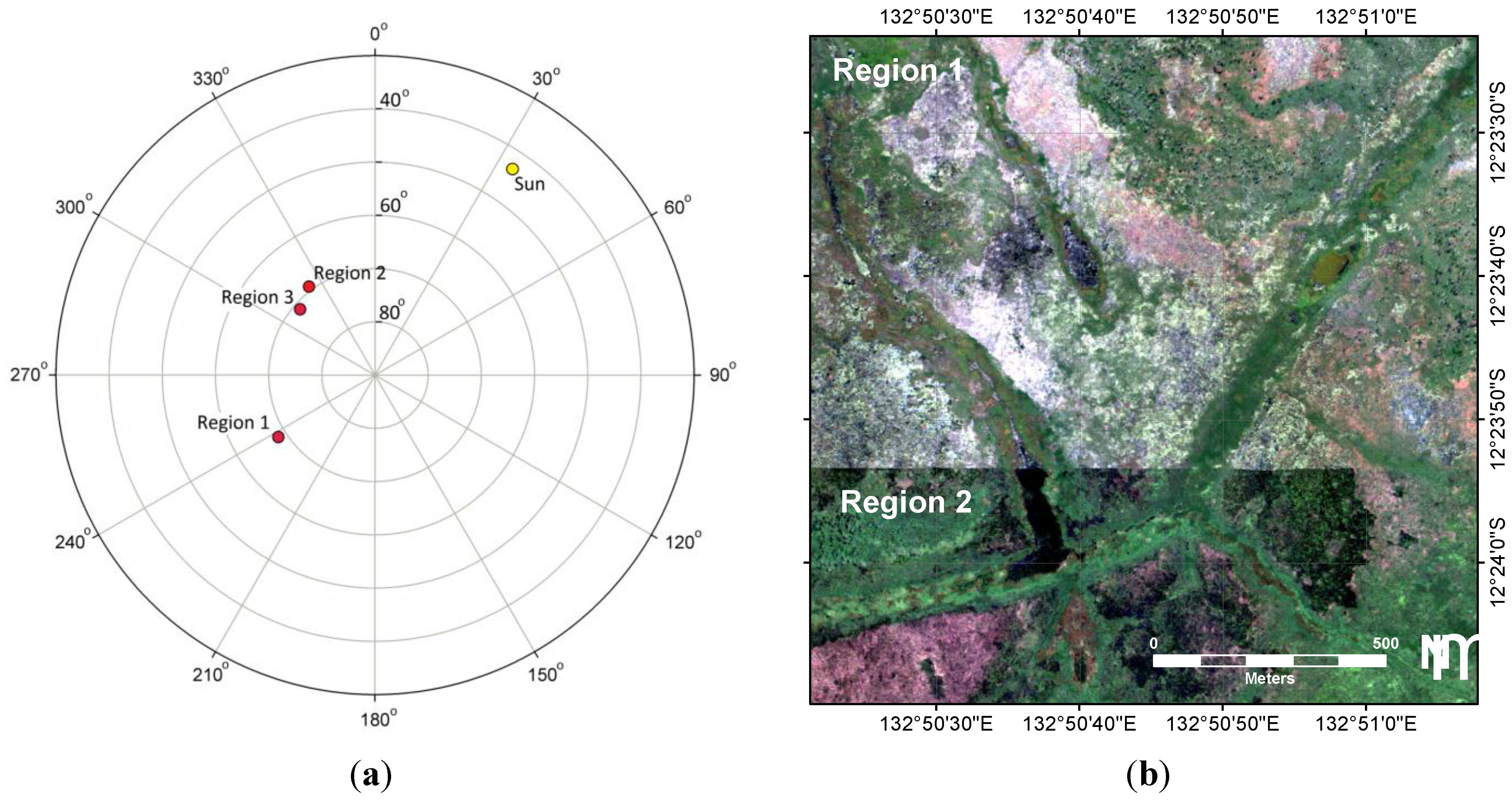
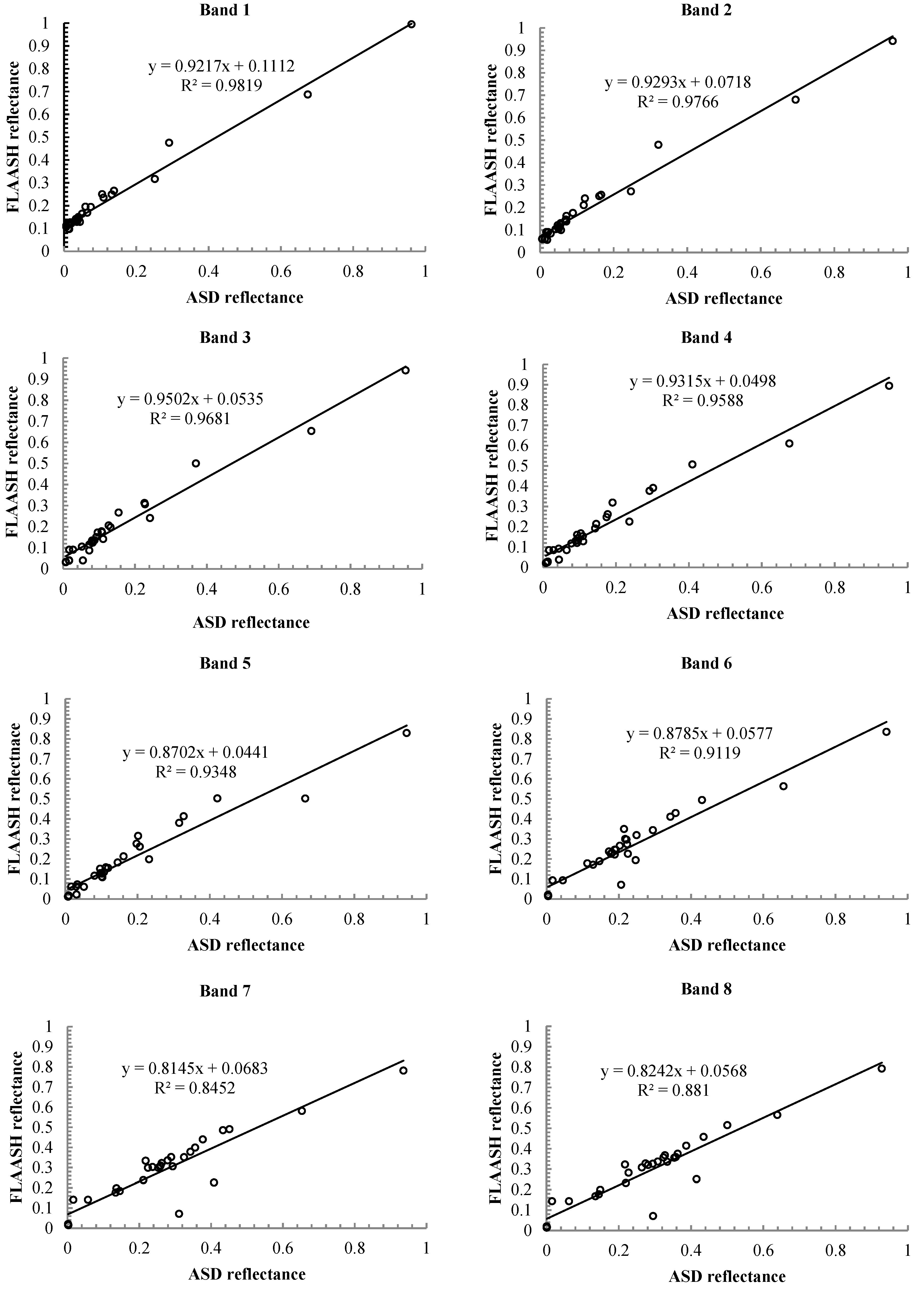
Due to sun glint, it was difficult to discern open water and floating vegetation within Region 1. In addition, due to changes in reflectance associated with the view angle, the class rulesets developed for Regions 2 and 3 did not satisfactorily detect the classes in Region 1. This required a modified set of rules and threshold values for Region 1. Although the FLAASH atmospheric correction algorithm accounts for view angle, it is difficult to correct for sun glint on floodplains. Ensuring the imagery is captured along a single path will prevent this issue from reoccurring.
Floodplain boundary delineation was useful to limit classification to the relevant vegetation communities and would have not been possible using only WV-2 imagery due to spectral similarities between floodplain and non-floodplain surfaces. The inclusion of DEM data was useful in providing an initial delineation of the floodplain boundary that could easily be manually adjusted. Both DEMs contain uncertainty in elevation, with the 30 m resolution DEM too coarse and the 10 m DEM suffering from vegetation effects in the northern section. Consequently, a manual modification of the boundary was necessary based upon visual interpretation of the multispectral imagery.
The classification of HSR imagery does lead to an interesting problem associated with the scale and resolution. The high resolution (GSD = 2 m) of the WV-2 imagery produced a map scale including a level of detail that may mean some small objects only contained one individual of a species. For example, an object of 25 pixels classified as Melaleuca open forest might be a single tree. Objects of that scale may not be suitable for broader landscape analysis where community level classification is needed, therefore classes would need to be more specific to describe an individual organism of a single species. The hierarchical grouping of objects within GEOBIA would be one means to address this issue.
The vegetation maps were representative of the vegetation that existed on the floodplain in May 2010. The seasonal variation that is known to occur [9,33] has not been captured within this map, such as changes in community composition associated with the varying water level and soil moisture in the floodplain. The amount and periodicity of rainfall varies annually leading to different water levels and soil moisture availability means community distributions can vary greatly within and between years. Although previously undertaken for the 2006 dry season using a time-series of four sets of Landsat imagery [9], mapping vegetation at this temporal scale can be problematic. For a large interval of the year, optical satellite data of a suitable quality is unavailable due to either cloud cover or smoke haze and, as the year progresses, so does the area of fire-affected land cover. In addition, using HSR data from a commercial satellite means data collection of such temporal intensity would be cost prohibitive. Although it was not possible to directly compare the results of this study to the map of Boyden et al. [9] due to temporal, spatial and methodological differences, a couple of observations can be made. Due to the higher spatial resolution of the imagery, the map produced for this study had better delineation of class boundaries. This map however had less success at discriminating between the various grass classes because unlike Boyden et al. [9], this study was not able to analyse the temporal changes in spectral responses of grass dominated land cover.
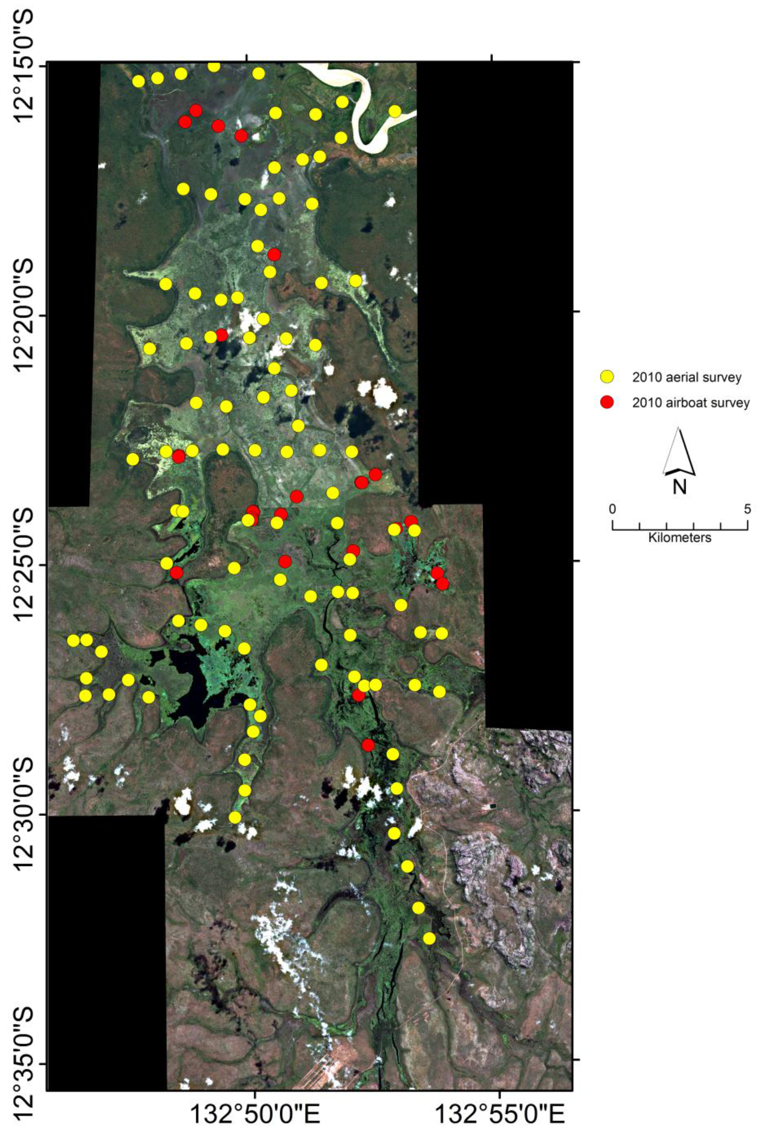
For reference data, it would be preferable to have more points to increase the rigour of the accuracy assessment, as several of the classes have limited reference data. However, gaining sufficient reference data is difficult using standard observation techniques due to accessibility and hazard issues associated with the remote environment, and resource limitations. For HSR image analysis, a number of studies have used the visual analysis of the base imagery to provide sufficient reference data for ground truthing providing what has been referred to as a pseudo accuracy assessment [53]. While this may be possible to undertake for easily discernible land covers, again, spectrally and texturally similar vegetation may be difficult to differentiate resulting in error, and bias may also be introduced by user influence [59]. New techniques for reference data collection using helicopter-based GPS enabled videography and still photography at higher spatial resolutions than the satellite imagery have been trialed for subsequent data captures to enable an increased number of reference sites relative to field sampling effort.

5. Conclusions

This research tests the application of a decision tree-based GEOBIA for mapping floodplain vegetation using WorldView-2 high spatial resolution imagery and ancillary data produced a vegetation map of the Magela Creek floodplain for May 2010. Based on the confusion matrix built using the field reference data, the overall accuracy of the decision tree classification was 78%. Half the overall disagreement was quantity disagreement, with the remainder mostly being exchange with the majority of error being associated with confusion between grass dominant classes that were spectrally similar but different species composition. The overall accuracy of the RF classification was 64% with half the overall disagreement being quantity disagreement and the remainder mostly exchange. Again there was mostly confusion between the grass classes that were spectrally similar. Results of the z-test and McNemar’s test showed that there was a significant difference between the results of the DT and RF classifications and that for this project the DT method clearly outperformed the RF. These results suggests that the method may be useful for classifying wetlands that are difficult to map using supervised classification methods, such as RF.
The maps, however, are representative of a point in time and do not account for any temporal variability (either seasonal or annual) in the extent and distribution of the vegetation communities on the floodplain.
Due to the performance of the DT approach, the method described here (with the Pseudorpahis, Hymenachne and Pseudorpahis/Hymenachne classes merged into a single class) has been applied to mapping the floodplain vegetation in over a time-series (2010–2013) to monitor the annual variation in distribution and extent of the communities and changes in open water [48]. This work forms an integral component of an operational landscape scale off-site monitoring program for the rehabilitation of Ranger Uranium Mine.

Acknowledgments

Parks Australia for contributing towards the WorldView-2 image capture. James Boyden, Grant Staben and Annamarie Berraldo for assistance in collecting the field reference data.

Author Contributions

Timothy Whiteside wrote the manuscript, undertook pre-processing of the imagery, developed the decision tree classification model, undertook both the decision tree and Random Forests classifications and conducted accuracy assessment. Renée Bartolo designed the research, collected the field reference data and contributed to manuscript writing and revision.

Conflicts of Interest

The authors declare no conflict of interest.

References

  1. Franklin, P.; Dunbar, M.; Whitehead, P. Flow controls on lowland river macrophytes: A review. Sci. Total Environ. 2008, 400, 369–378. [Google Scholar] [CrossRef] [PubMed]
  2. Adam, E.; Mutanga, O.; Rugege, D. Multispectral and hyperspectral remote sensing for identification and mapping of wetland vegetation: A review. Wetl. Ecol. Manag. 2010, 18, 281–296. [Google Scholar] [CrossRef]
  3. Klemas, V. Remote sensing of wetlands: Case studies comparing practical techniques. J. Coast. Res. 2011, 27, 418–427. [Google Scholar] [CrossRef]
  4. Klemas, V. Remote sensing of emergent and submerged wetlands: an overview. Int. J. Remote Sens. 2013, 34, 1–35. [Google Scholar] [CrossRef]
  5. Ozesmi, S.L.; Bauer, M.E. Satellite remote sensing of wetlands. Wetl. Ecol. Manag. 2002, 10, 381–402. [Google Scholar] [CrossRef]
  6. Silva, T.F.; Costa, M.F.; Melack, J.; Novo, E.L.M. Remote sensing of aquatic vegetation: Theory and applications. Environ. Monit. Assess. 2008, 140, 131–145. [Google Scholar] [CrossRef] [PubMed]
  7. Baker, C.; Lawrence, R.; Montagne, C.; Patten, D. Mapping wetlands and riparian areas using Landsat ETM+ imagery and decision-tree-based models. Wetlands 2006, 26, 465–474. [Google Scholar] [CrossRef]
  8. Wright, C.; Gallant, A. Improved wetland remote sensing in Yellowstone National Park using classification trees to combine TM imagery and ancillary environmental data. Remote Sens. Environ. 2007, 107, 582–605. [Google Scholar] [CrossRef]
  9. Boyden, J.; Joyce, K.E.; Boggs, G.; Wurm, P. Object-based mapping of native vegetation and para grass (Urochloa mutica) on a monsoonal wetland of Kakadu NP using a Landsat 5 TM dry-season time series. J. Spat. Sci. 2013, 58, 53–77. [Google Scholar] [CrossRef]
  10. Harvey, K.; Hill, G. Vegetation mapping of a tropical freshwater swamp in the Northern Territory, Australia: A comparison of aerial photography, Landsat TM and SPOT satellite imagery. Int. J. Remote Sens. 2001, 22, 2911–2925. [Google Scholar] [CrossRef]
  11. Szantoi, Z.; Escobedo, F.; Abd-Elrahman, A.; Smith, S.; Pearlstine, L. Analyzing fine-scale wetland composition using high resolution imagery and texture features. Int. J. Appl. Earth Obs. Geoinf. 2013, 23, 204–212. [Google Scholar] [CrossRef]
  12. Ward, D.P.; Petty, A.; Setterfield, S.A.; Douglas, M.M.; Ferdinands, K.; Hamilton, S.K.; Phinn, S. Floodplain inundation and vegetation dynamics in the Alligator Rivers region (Kakadu) of northern Australia assessed using optical and radar remote sensing. Remote Sens. Environ. 2014, 147, 43–55. [Google Scholar] [CrossRef]
  13. Basham May, A.M.; Pinder, J.; Kroh, G. A comparison of Landsat Thematic Mapper and SPOT multi-spectral imagery for the classification of shrub and meadow vegetation in northern California, USA. Int. J. Remote Sens. 1997, 18, 3719–3728. [Google Scholar] [CrossRef]
  14. McCarthy, J.; Gumbricht, T.; McCarthy, T. Ecoregion classification in the Okavango Delta, Botswana from multitemporal remote sensing. Int. J. Remote Sens. 2005, 26, 4339–4357. [Google Scholar] [CrossRef]
  15. Blaschke, T. Object based image analysis for remote sensing. ISPRS J. Photogramm. Remote Sens. 2010, 65, 2–16. [Google Scholar] [CrossRef]
  16. Blaschke, T.; Hay, G.J.; Kelly, M.; Lang, S.; Hofmann, P.; Addink, E.; Queiroz Feitosa, R.; van der Meer, F.; van der Werff, H.; van Coillie, F.; et al. Geographic Object-Based Image Analysis—Towards a new paradigm. ISPRS J. Photogramm. Remote Sens. 2014, 87, 180–191. [Google Scholar] [CrossRef] [PubMed]
  17. Kettig, R.L.; Landgrebe, D.A. Classification of multispectral image data by extraction and classification of homogeneous objects. IEEE Trans. Geosci. Electron. 1976, 14, 19–26. [Google Scholar] [CrossRef]
  18. Benz, U.; Hofmann, P.; Willhauck, G.; Lingenfelder, I.; Heynen, M. Multi-resolution, object-oriented fuzzy analysis of remote sensing data for GIS-ready information. ISPRS J. Photogramm. Remote Sens. 2004, 58, 239–258. [Google Scholar] [CrossRef]
  19. Lennartz, S.P.; Congalton, R.G. Classifying and mapping forest cover types using IKONOS imagery in the norteastern United States. In Proceedings of the ASPRS Annual Conference, Denver, CO, USA, 23–28 May 2004. unpaginated CD-ROM.
  20. Hay, G.J.; Blaschke, T.; Marceau, D.J.; Bouchard, A. A comparison of three image-object methods for the multi-scale analysis of landscape structure. ISPRS J. Photogramm. Remote Sens. 2003, 57, 327–345. [Google Scholar] [CrossRef]
  21. Hay, G.J.; Castilla, G. Geographic Object-Based Image Analysis (GEOBIA): A new name for a new discipline. In Object-based image analysis-Spatial Concepts for Knowledge-Driven Remote Sensing Applications; Blaschke, T., Lang, S., Hay, G.J., Eds.; Springer Verlag: Berlin, Germany, 2008; pp. 75–89. [Google Scholar]
  22. Breiman, L. Random forests. Mach. Learn. 2001, 45, 5–32. [Google Scholar] [CrossRef]
  23. Liaw, A.; Wiener, M. Classification and regression by random Forest. R news 2002, 2, 18–22. [Google Scholar]
  24. Gislason, P.O.; Benediktsson, J.A.; Sveinsson, J.R. Random Forests for land cover classification. Pattern Recognition Lett. 2006, 27, 294–300. [Google Scholar] [CrossRef]
  25. Cutler, D.R.; Edwards, T.C., Jr.; Beard, K.H.; Cutler, A.; Hess, K.T.; Gibson, J.; Lawler, J.J. Random forests for classification in ecology. Ecology 2007, 88, 2783–2792. [Google Scholar] [CrossRef] [PubMed]
  26. Dorigo, W.; Lucieer, A.; Podobnikar, T.; Čarni, A. Mapping invasive Fallopia japonica by combined spectral, spatial, and temporal analysis of digital orthophotos. Int. J. Appl. Earth Obs. Geoinf. 2012, 19, 185–195. [Google Scholar] [CrossRef]
  27. Lawrence, R.L.; Wood, S.D.; Sheley, R.L. Mapping invasive plants using hyperspectral imagery and Breiman Cutler classifications (randomForest). Remote Sens. Environ. 2006, 100, 356–362. [Google Scholar] [CrossRef]
  28. Pal, M. Random forest classifier for remote sensing classification. Int. J. Remote Sens. 2005, 26, 217–222. [Google Scholar] [CrossRef]
  29. Finlayson, C.M.; Lowry, J.; Grazia Bellio, M.; Nou, S.; Pidgeon, R.W.J.; Walden, D.J.; Humphrey, C.; Fox, G. Biodiversity of the wetlands of the Kakadu Region, northern Australia. Aquat. Sci. 2006, 68, 374–399. [Google Scholar] [CrossRef]
  30. Bayliss, P.; Yeomans, K.M. Seasonal distribution and abundance of magpie geese, Anseranus-Semipalmata Latham, in the Northern Territory and their relationship to habitat, 1983–1986. Aust. Wildl. Res. 1990, 17, 15–38. [Google Scholar] [CrossRef]
  31. Bellio, M.G.; Bayliss, P.; Dostine, P. Landscape-Scale Analysis of the Value of Waterbirds in the Alligator Rivers Region, Northern Australia; Internal Report 445; Supervising Scientist: Darwin, Australia, 2004. [Google Scholar]
  32. Bayliss, P.; van Dam, R.A.; Bartolo, R.E. Quantitative ecological risk assessment of the Magela Creek floodplain in Kakadu National Park, Australia: comparing point source risks from the Ranger Uranium Mine to diffuse landscape-scale risks. Hum. Ecol. Risk Assess. 2012, 18, 115–151. [Google Scholar] [CrossRef]
  33. Finlayson, C.M.; Bailey, B.J.; Cowie, I.D. Macrophyte Vegetation of the Magela Creek Flood Plain, Alligator Rivers Region, Northern Territory; Research Report 5; Supervising Scientist for the Alligator Rivers Region: Canberra, Austrilia, 1989; p. 38. [Google Scholar]
  34. Williams, A. Vegetation and stream pattern as indicators of water movement on the Magela Floodplain, Northern Territory. Aust. J. Ecol. 1979, 4, 239–247. [Google Scholar] [CrossRef]
  35. Saynor, M.J.; Erskine, W.D. Classification of river reaches on the little disturbed East Alligator River, northern Australia. Int. J. Geosci. 2013, 4, 53–65. [Google Scholar] [CrossRef]
  36. Boyden, J.M.; Walden, D.J.; Bartolo, R.; Bayliss, P. Utility of VHR remote sensing data for landscape assessment of the environmental weed para grass [Urochloa mutica, (Forssk)]. In Proceedings of Asian Conference on Remote Sensing, Kuala Lumpur, Malaysia, 12–16 November, 2007; Malaysian Centre for Remote Sensing and Ministry of Science (MACRES), Technology and Innovation (MOSTI), Malaysia: Kuala Lumpur, Malaysia, 2007. [Google Scholar]
  37. Updike, T.; Comp, C. Radiometric Use of WorldView-2 Imagery; DigitalGlobe: Longmont, CO, USA, 2010; p. 17. [Google Scholar]
  38. Clevers, J.; De Jong, S.; Epema, G.; Van der Meer, F.; Bakker, W.; Skidmore, A.; Scholte, K. Derivation of the red edge index using the MERIS standard band setting. Int. J. Remote Sens. 2002, 23, 3169–3184. [Google Scholar] [CrossRef]
  39. Horler, D.N.H.; Dockray, M.; Barber, J. The red edge of plant leaf reflectance. Int. J. Remote Sens. 1983, 4, 273–288. [Google Scholar] [CrossRef]
  40. Filella, I.; Penuelas, J. The red edge position and shape as indicators of plant chlorophyll content, biomass and hydric status. Int. J. Remote Sens. 1994, 15, 1459–1470. [Google Scholar] [CrossRef]
  41. Mutanga, O.; Adam, E.; Cho, M.A. High density biomass estimation for wetland vegetation using WorldView-2 imagery and random forest regression algorithm. Int. J. Appl. Earth Obs. Geoinf. 2012, 18, 399–406. [Google Scholar] [CrossRef]
  42. Whiteside, T.; Bartolo, R.; Pfitzner, K.; Staben, G. Geometric and Radiometric Correction of WorldView-2 Satellite Imagery; Internal Report 617; Supervising Scientist: Darwin, Australia, 2013. [Google Scholar]
  43. Staben, G.; Pfitzner, K.; Bartolo, R.; Lucieer, A. Empirical line calibration of WorldView-2 satellite imagery to reflectance data: Using quadratic prediction equations. Remote Sens. Lett. 2012, 3, 521–530. [Google Scholar] [CrossRef]
  44. Matthew, M.; Adler-Golden, S.; Berk, A.; Felde, G.; Anderson, G.; Gorodetzky, D.; Paswaters, S.; Shippert, M. Atmospheric correction of spectral imagery: evaluation of the FLAASH algorithm with AVIRIS data. Proc. SPIE 2003, 5093, 474–482. [Google Scholar]
  45. Baatz, M.; Schäpe, A. Multiresolution segmentation - an optimization approach for high quality multi-scale image segmentation. In Angewandte Geographische Informationsverarbeitung XII; Strobl, J., Blaschke, T., Griesebner, G., Eds.; Wichmann-Verlag: Heidelberg, Germany, 2000; pp. 12–23. [Google Scholar]
  46. Willhauck, G.; Schneider, T.; De Kok, R.; Ammer, U. Comparison of object-oriented classification techniques and standard image analysis for the use of change detection between SPOT multispectral satellite images and aerial photos. In Proceedings of the XIX ISPRS Congress, Amsterdam, The Netherlands, 16–22 July 2000.
  47. Whiteside, T.G.; Bartolo, R.E. Use of WorldView-2 time series to establish a wetland monitoring program for potential offsite impacts of mine site rehabilitation. Int. J. Appl. Earth Obs. Geoinf. 2015, 42, 24–37. [Google Scholar] [CrossRef]
  48. Hnatiuk, R.J.; Thackway, R.; Walker, J. Vegetation. In Australian Soil and Land Survey Field Handbook, 3rd ed.; CSIRO: Melbourne, Austrilia, 2009; pp. 73–125. [Google Scholar]
  49. Powers, R.P.; Hay, G.J.; Chen, G. How wetland type and area differ through scale: A GEOBIA case study in Alberta’s Boreal Plains. Remote Sens. Environ. 2012, 117, 135–145. [Google Scholar] [CrossRef]
  50. Bunting, P.; Lucas, R. The delineation of tree crowns in Australian mixed species forests using hyperspectral Compact Airborne Spectrographic Imager (CASI) data. Remote Sens. Environ. 2006, 101, 230–248. [Google Scholar] [CrossRef]
  51. Rouse, J.W.; Haas, R.H.; Schell, J.A.; Deering, D.W. Monitoring vegetation systems in the Great Plains with ERTS. In Proceedings of 3rd ERTS Symposium, NASA, Washington, USA, 1973; pp. 309–317.
  52. Huete, A.R.; Didan, K.; Miura, T.; Rodriguez, E.P.; Gao, X.; Ferreira, L.G. Overview of the radiometric and biophysical performance of the MODIS vegetation indices. Remote Sens. Environ. 2002, 83, 195–213. [Google Scholar] [CrossRef]
  53. Congalton, R.G.; Green, K. Assess. Accuracy Remotely Sensing Data: Principles and Practices, 2nd ed.; CRC Press: Boca Raton, FL, USA, 2009; p. 183. [Google Scholar]
  54. Cohen, J. A coefficient of agreement for nominal scales. Educ. Psychol. Meas. 1960, 20, 37–46. [Google Scholar] [CrossRef]
  55. Pontius, R.G.; Millones, M. Death to Kappa: Birth of quantity disagreement and allocation disagreement for accuracy assessment. Int. J. Remote Sens. 2011, 32, 4407–4429. [Google Scholar] [CrossRef]
  56. Pontius, R.G.; Santacruz, A. Quantity, exchange, and shift components of difference in a square contingency table. Int. J. Remote Sens. 2014, 35, 7543–7554. [Google Scholar] [CrossRef]
  57. De Leeuw, J.; Jia, H.; Yang, L.; Liu, X.; Schmidt, K.; Skidmore, A.K. Comparing accuracy assessments to infer superiority of image classification methods. Int. J. Remote Sens. 2006, 27, 223–232. [Google Scholar] [CrossRef]
  58. Dingle Robertson, L.; King, D.J. Comparison of pixel- and object-based classification in land cover mapping. Int. J. Remote Sens. 2011, 32, 1505–1529. [Google Scholar] [CrossRef]
  59. Foody, G.M. Status of land cover classification accuracy assessment. Remote Sens. Environ. 2002, 80, 185–201. [Google Scholar] [CrossRef]

