
aTrunk—An ALS-Based Trunk Detection Algorithm


Abstract
:
1. Introduction
1.1. Relevance
1.2. State of the Art
1.3. Related Work
1.4. Objective
2. Materials and Methods
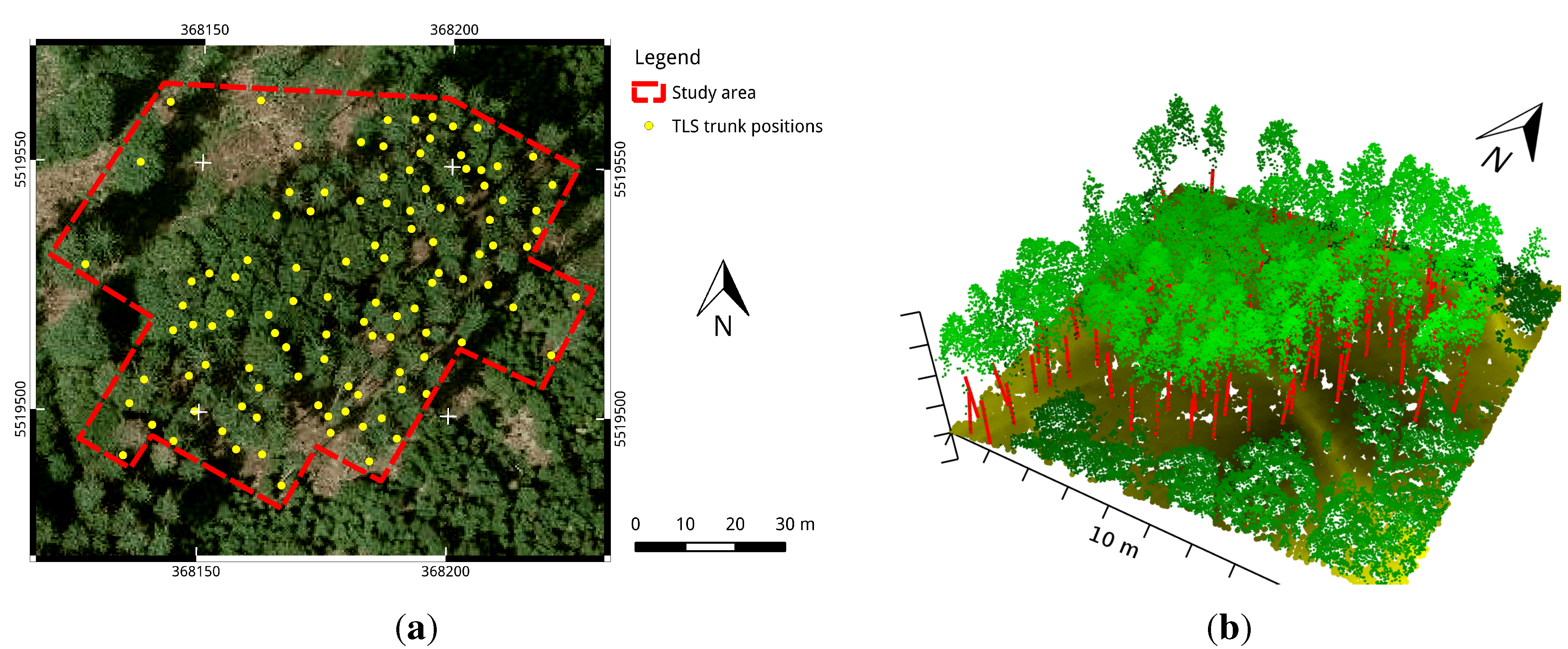
2.1. Study Area
2.2. ALS Data
2.3. Validation Data
2.4. Methods
2.4.1. Preprocessing
2.4.2. Assumptions on Trunk Representation
- widely spatially separable from the crown portion and the ground covering vegetation.
- moderately surrounded by points associated with branches, foliage or other objects.
- arranged in a straight line, which is oriented along the growth direction of the trunk. The maximum deviation from this line depends on the length of the trunk, for example, caused by irregular growth or branching.
- largely uniformly distributed in growth direction of the trunk, which is substantiated in the spatial resolution of the ALS data.
2.5. Trunk Detection Algorithm

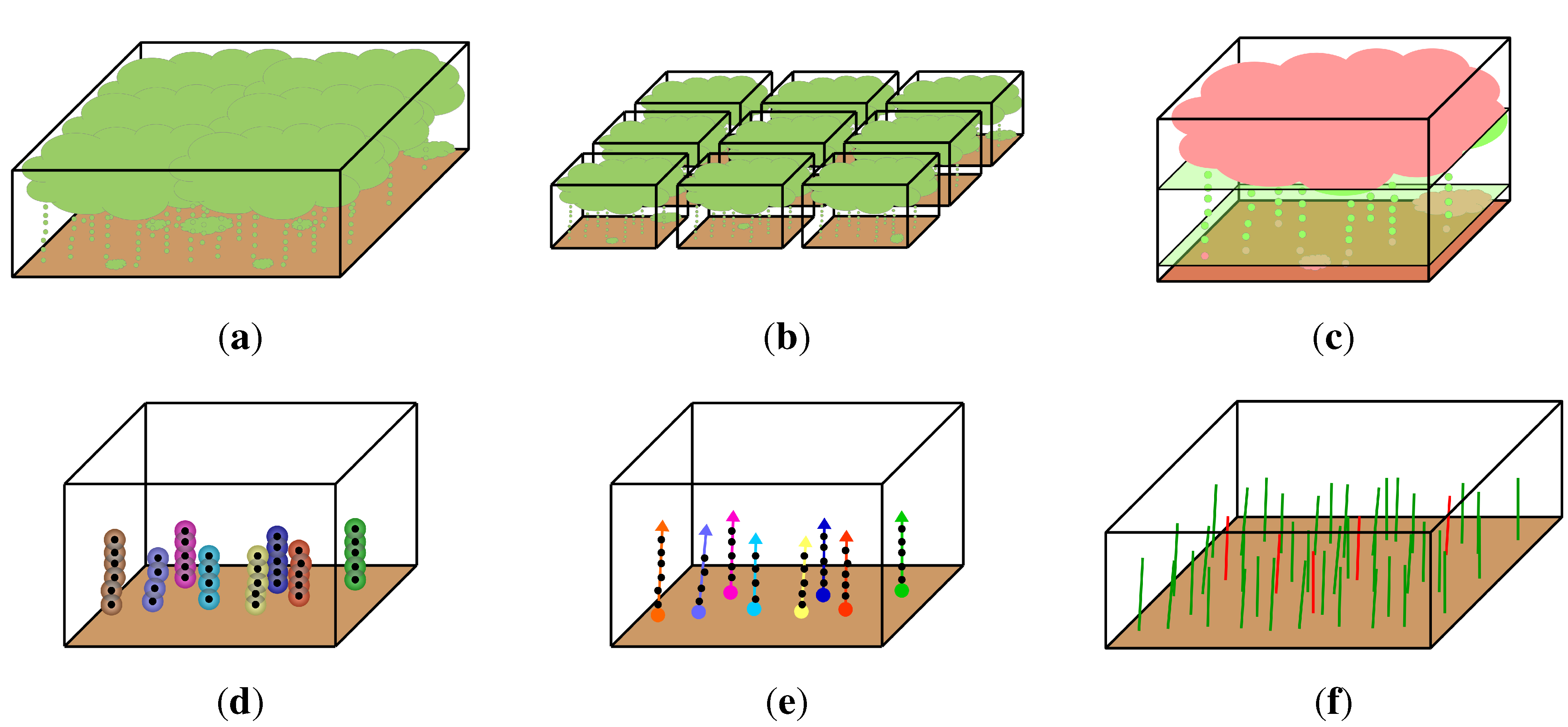
2.5.1. Divide & Conquer
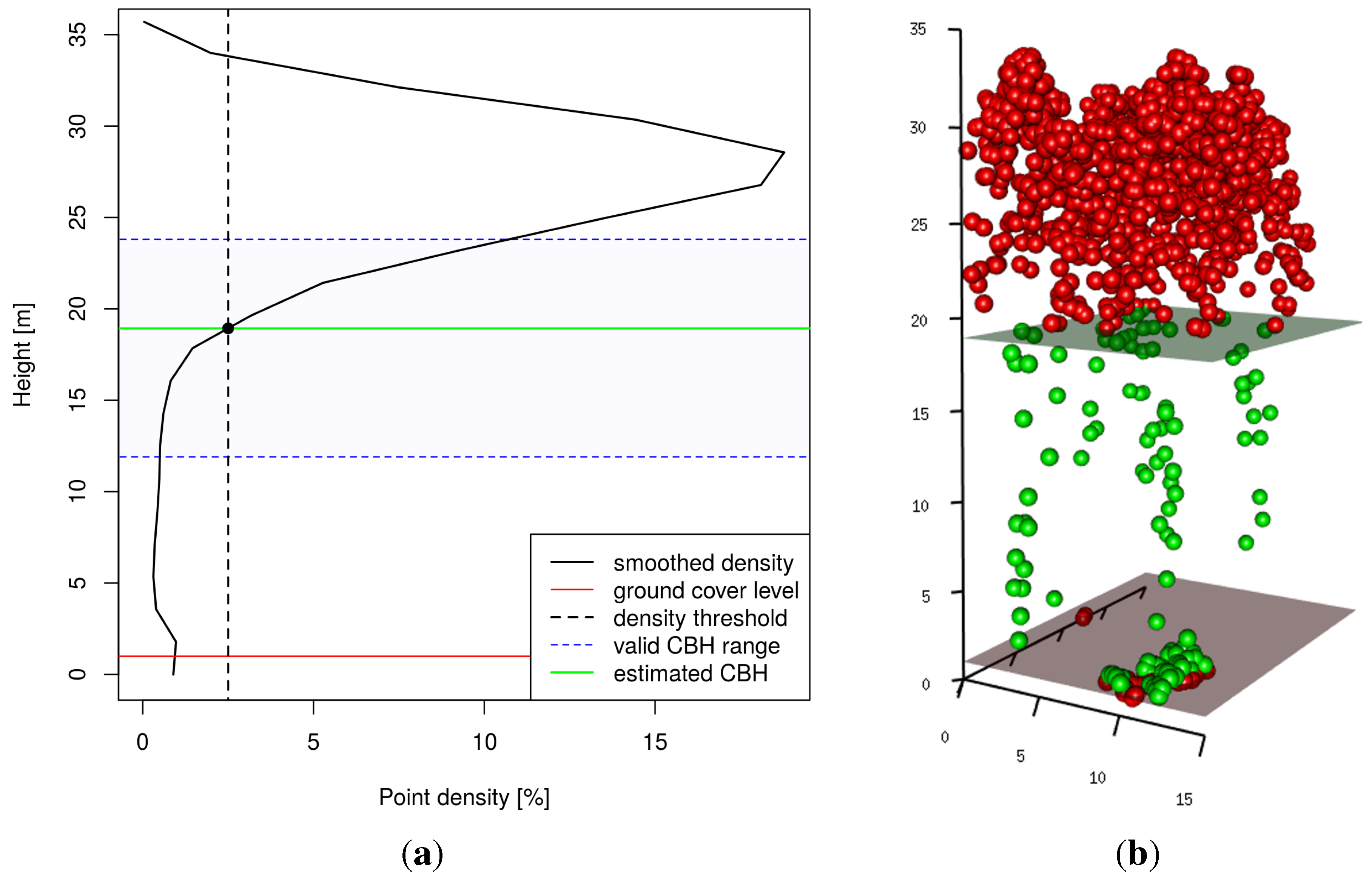
2.5.2. Separation of the Trunk Section
2.5.3. Clustering
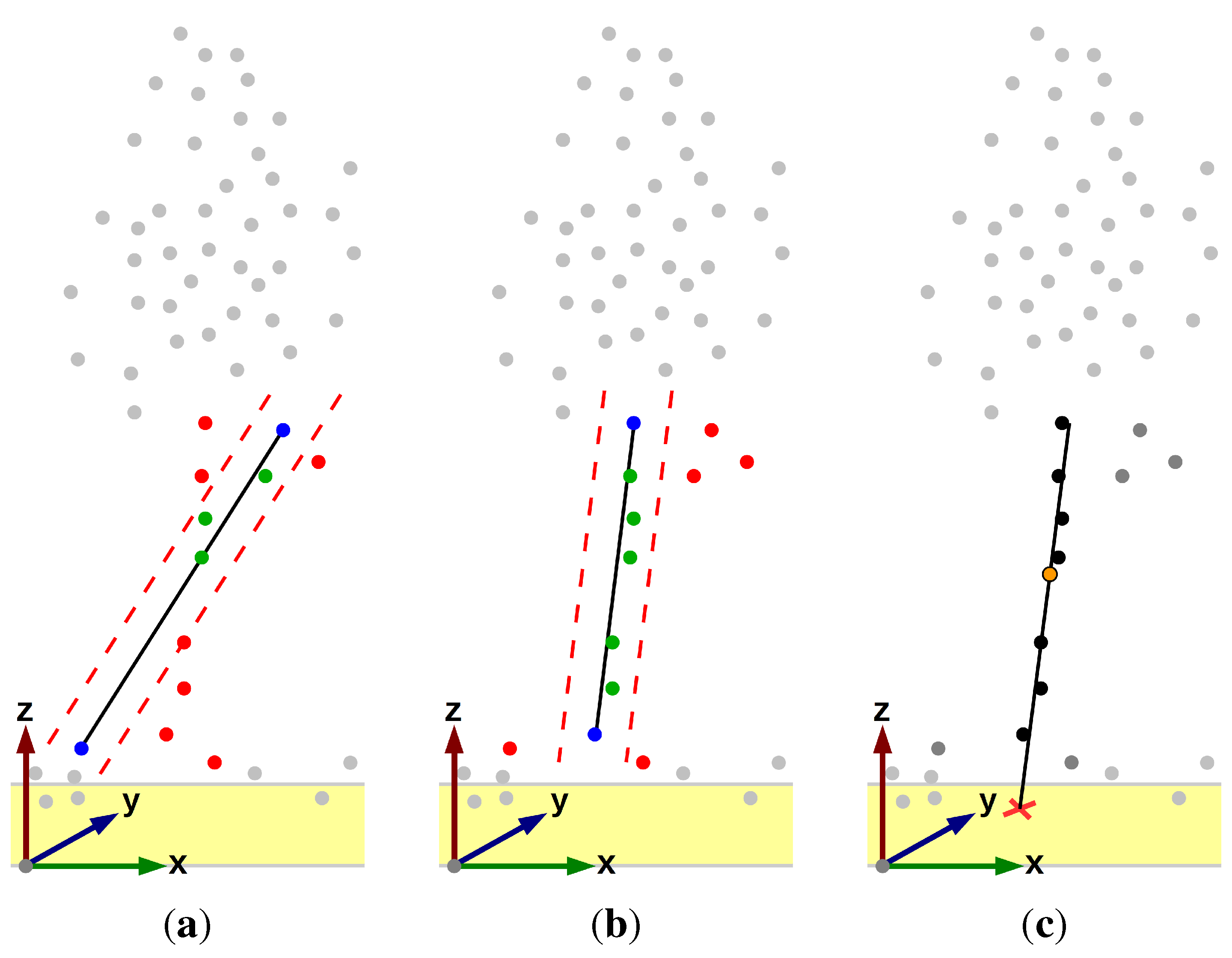
2.5.4. Trunk Model
- it contains enough points to ensure an accurate adaptation but unlikely false detections.
- it contains only some points, because it is assumed that a high number of neighboured points is probably caused by leaves or branches. The value ρ corresponds to the point density of the sample.
- the range of z is large enough to contain a trunk.
- the ratio between the z-range (height) and xy-range (width) is comprehensible.
- the zenith angle of the trunk is reasonable.
- the model has a favourable ratio between model-supporting points and outliers.
- the points associated with the trunk are largely uniformly distributed in direction.
2.5.5. Merge Duplicated Trunks

2.6. Trunk Model Properties
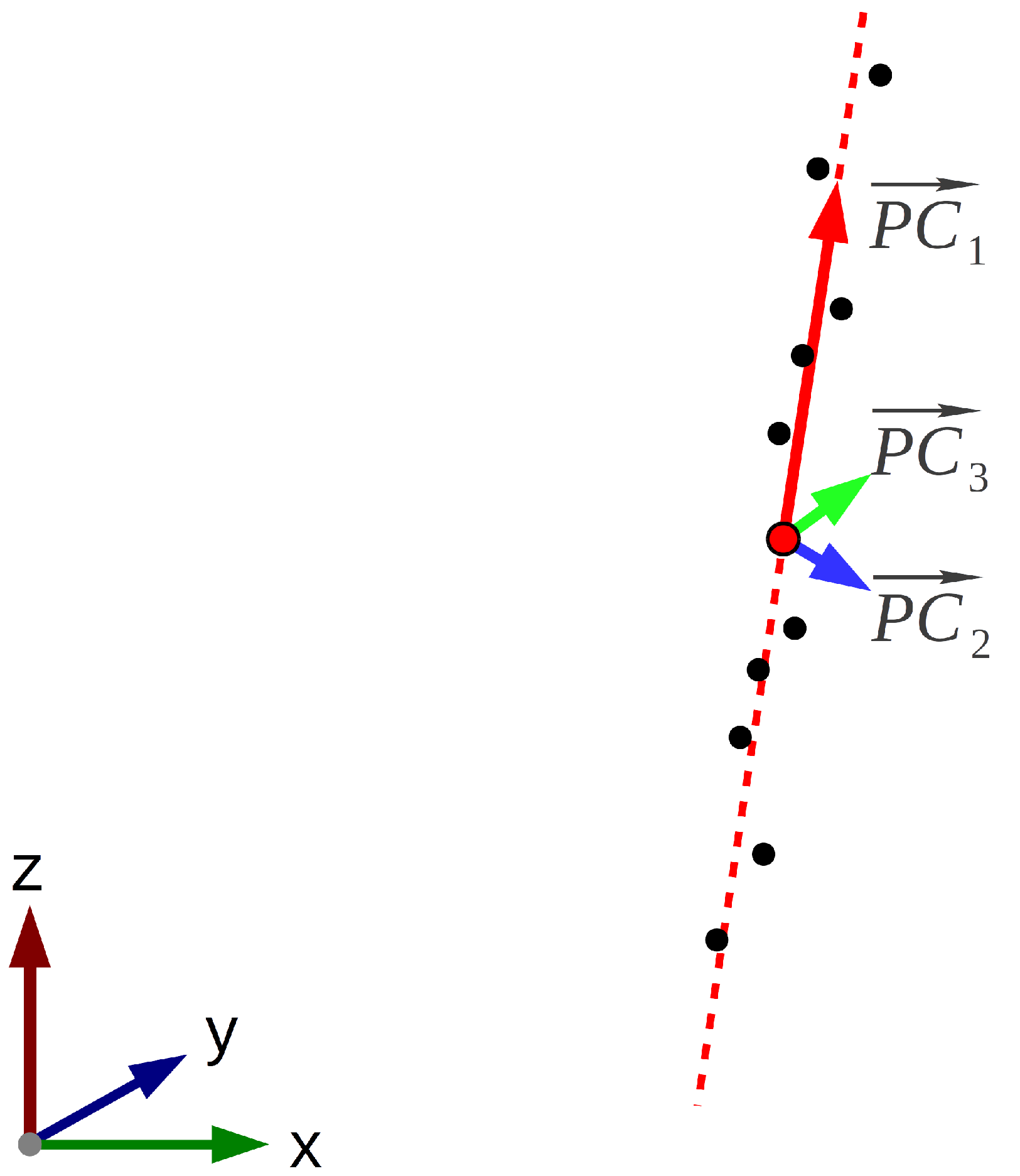
2.6.1. Principal Component Model
2.6.2. Trunk Orientation
2.6.3. Position
2.6.4. Trunk Height
2.6.5. Quality Criteria
2.7. Methods of Evaluation

| Parameter Name | Values’ Range | Unit | Description | Value in This Study | Reference Section |
|---|---|---|---|---|---|
| () | – | Minimum number of points assumed to form a trunk | 4 | 2.5.4 | |
| () | – | Adaptive maximum number of points forming a trunk | 5.0 | 2.5.4 | |
| m | Width of the overlapping area | 5 | 2.5.1 | ||
| m | Maximum xy-size of a sample before trunk identification | 5 | 2.5.1 | ||
| – | Minimum ratio between z- and xy-range of a trunk | 3.0/1.0 | 2.5.4 | ||
| m | Minimum height of a trunk | 3.0 | 2.5.4 | ||
| () | ℝ | m | Maximum height of ground-covering vegetation | 1.0 | 2.5.2 |
| () | – | Assumed minimum relative crown base height | 0.35 | 2.5.2 | |
| () | – | Assumed maximum relative crown base height | 0.65 | 2.5.2 | |
| () | – | Default relative crown base height | 0.45 | 2.5.2 | |
| – | Threshold for crown base height estimation | 0.3 | 2.5.2 | ||
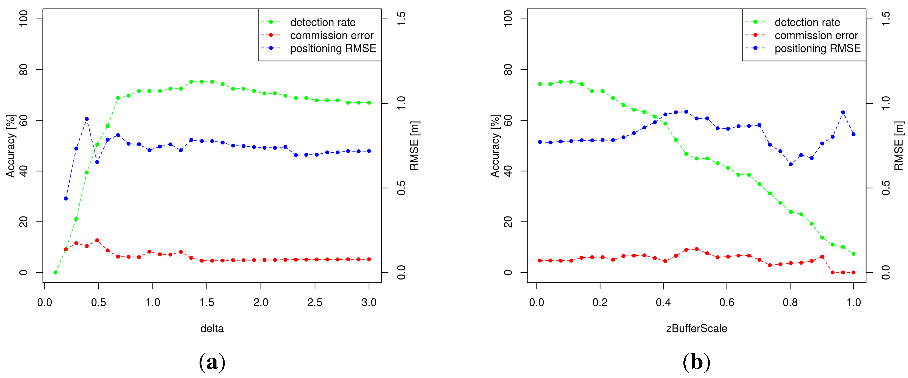
| (δ) | m | Maximum distance of clustering algorithm. | 1.5 | 2.5.3 | |
| ℕ | - | Minimum neighbours of a point in a cluster | 2 | 2.5.3 | |
| – | Scale factor of z-axis for 3D clustering | 0.1 | 2.5.3 | ||
| m | Expected maximum error per length of trunk | 0.07 | 2.5.4 | ||
| ◦ | Maximum assumed zenith angle of a trunk | 10 | 2.5.4 | ||
| – | Expected maximum ratio of and vs. | 0.7 | 2.5.4 | ||
| () | – | Assumed minimum unique distribution of the z-values | 0.001 | 2.6.5 | |
| m | Assumed minimum distance between two trunks | 1.8 | 2.5.5 |
3. Results and Discussion
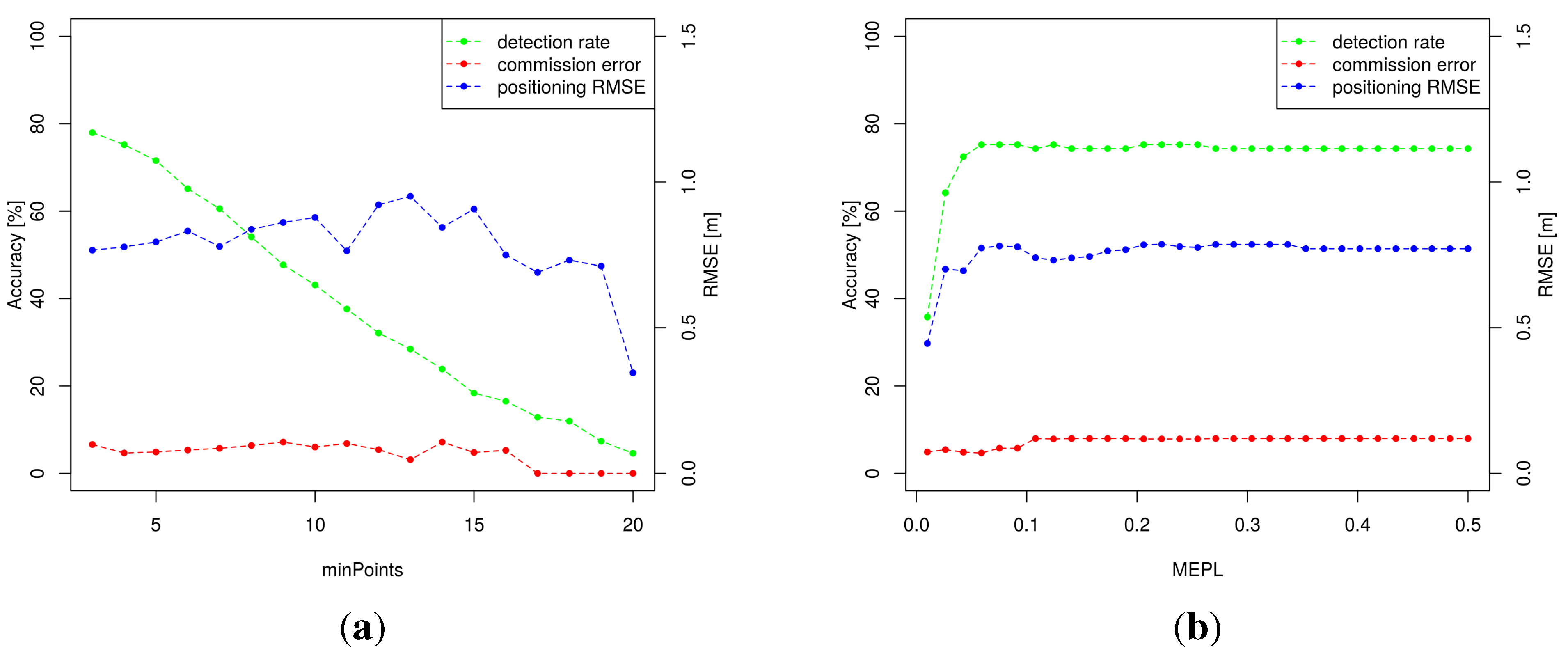
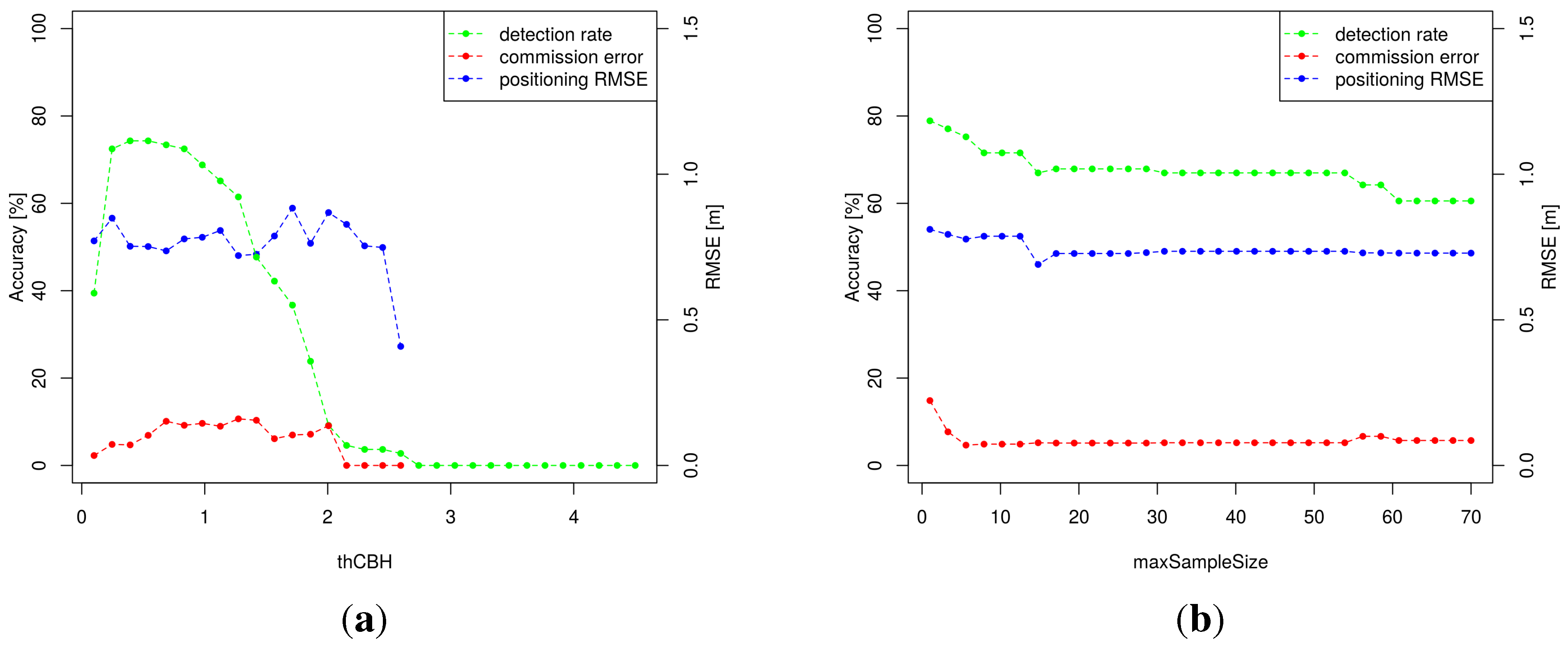
3.1. Sensitivity Analysis

| Group | Parameters | Expected Effect on Results |
|---|---|---|
| 1 | , , , | Control the computation effort |
| 2 | , , , | Control the trunk model accuracy |
| 3 | , , , , , | Rely on stand structure |
| 4 | δ, , | Control the clustering |
| 5 | , | Control the CBH estimation |
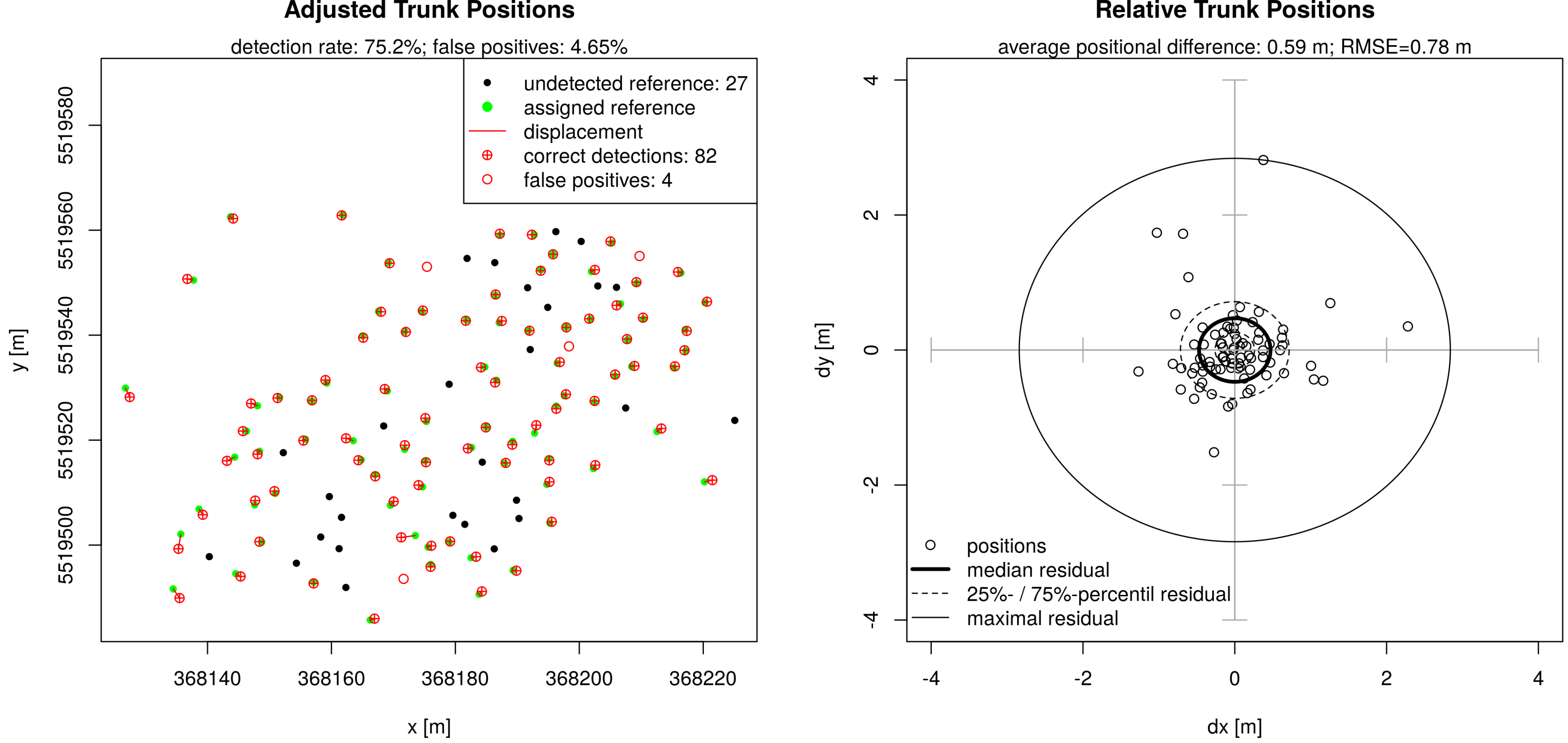
3.2. Evaluation
| Approach | Detection | Precision | Overall | Position Error | |
|---|---|---|---|---|---|
| Rate | Accuracy | Average | RMSE | ||
| watershed | 91% | 85% | 88% | 1.04m | 1.25m |
| aTrunk | 75% | 95% | 84% | 0.59m | 0.78m |
| matching | 69% | 96% | 80% | 0.64m | 0.82m |
| combined | 98% | 86% | 92% | 0.67m | 0.85m |

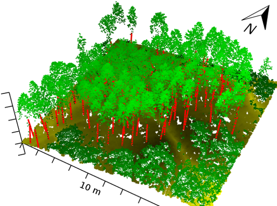
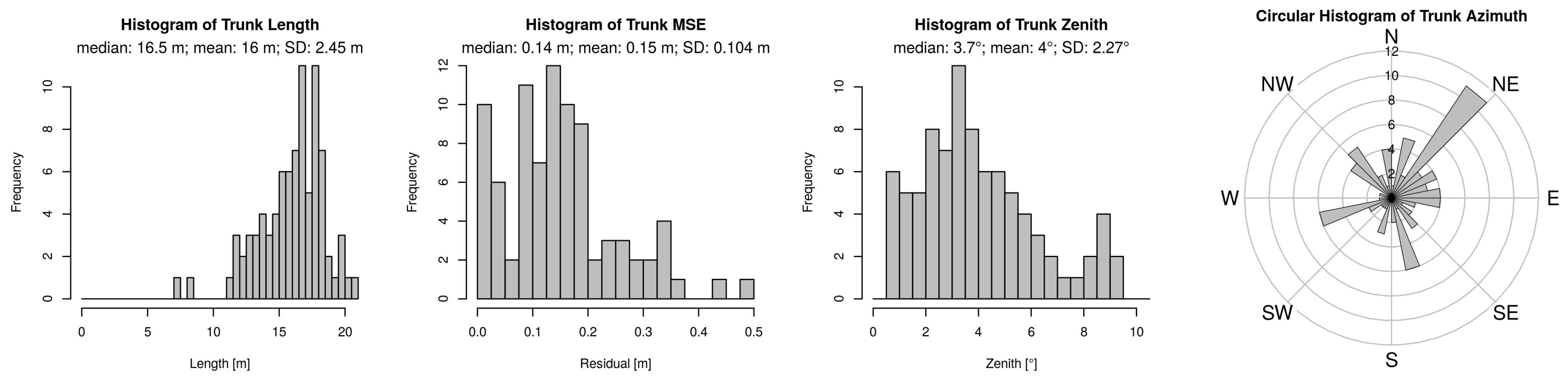
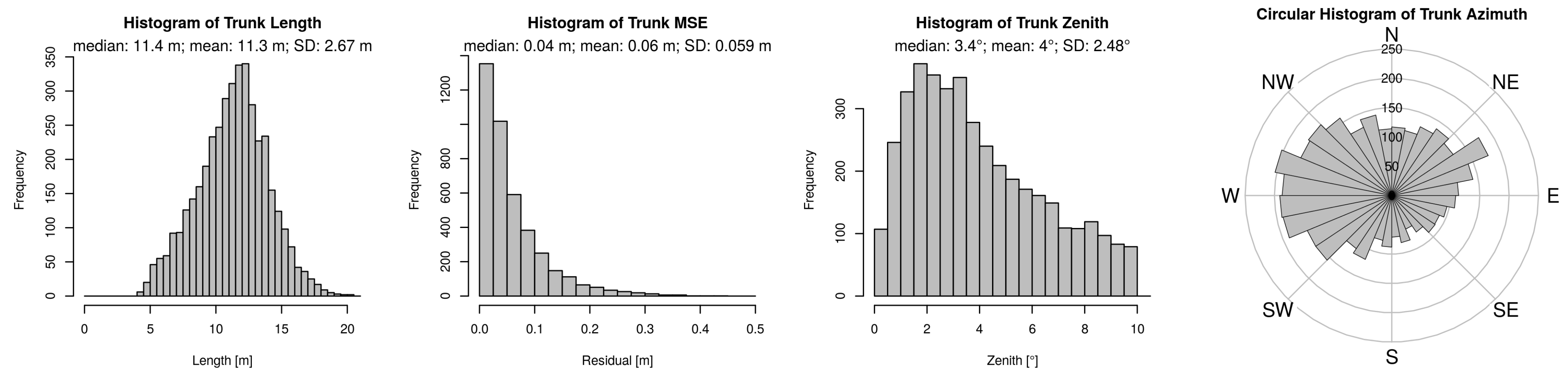
3.3. Modelling Results

3.4. Model Performance
3.5. Model Concept
4. Conclusions
Acknowledgments
Author Contributions
Conflicts of Interest
References
- Maes, W.H.; Fontaine, M.; Rongé, K.; Hermy, M.; Muys, B. A quantitative indicator framework for stand level evaluation and monitoring of environmentally sustainable forest management. Ecol. Indic. 2011, 11, 468–479. [Google Scholar] [CrossRef]
- Strîmbu, V.F.; Strîmbu, B.M. A graph-based segmentation algorithm for tree crown extraction using airborne LiDAR data. ISPRS J. Photogramm. Remote Sens. 2015, 104, 30–43. [Google Scholar] [CrossRef]
- Hyyppä, J.; Yu, X.; Hyyppä, H.; Vastaranta, M.; Holopainen, M.; Kukko, A.; Kaartinen, H.; Jaakkola, A.; Vaaja, M.; Koskinen, J.; et al. Advances in forest inventory using airborne laser scanning. Remote Sens. 2012, 4, 1190–1207. [Google Scholar] [CrossRef]
- Lafond, V.; Lagarrigues, G.; Cordonnier, T.; Courbaud, B. Uneven-aged management options to promote forest resilience for climate change adaptation: effects of group selection and harvesting intensity. Ann. For. Sci. 2013, 71, 173–186. [Google Scholar] [CrossRef]
- Kania, A.; Lindberg, E.; Schroiff, A.; Mücke, W.; Holmgren, J.; Pfeifer, N. Individual tree detection as input information for Natura 2000 habitat quality mapping. In Proceedings of the Remote Sensing and GIS for Monitoring Habitat Quality—RSGIS4HQ, Vienna, Austria, 24–25 September 2014.
- Holmgren, J.; Persson, A.; Söderman, U. Species identification of individual treesHolmgren by combining high resolution LiDAR data with multi-spectral images. Int. J. Remote Sens. 2008, 29, 1537–1552. [Google Scholar] [CrossRef]
- Ørka, H.O.; Na esset, E.; Bollandsås, O.M. Classifying species of individual trees by intensity and structure features derived from airborne laser scanner data. Remote Sens. Environ. 2009, 113, 1163–1174. [Google Scholar] [CrossRef]
- Yu, X.; Litkey, P.; Hyyppä, J.; Holopainen, M.; Vastaranta, M. Assessment of low density full-waveform airborne laser scanning for individual tree detection and tree species classification. Forests 2014, 5, 1011–1031. [Google Scholar] [CrossRef]
- Jakubowski, M.K.; Li, W.; Guo, Q.; Kelly, M. Delineating individual trees from LiDAR data: A comparison of vector-and raster-based segmentation approaches. Remote Sens. 2013, 5, 4163–4186. [Google Scholar] [CrossRef]
- Leiterer, R.; Mücke, W.; Hollaus, M.; Pfeifer, N.; Schaepman, M.E. Operational forest structure monitoring using airborne laser scanning. Photogramm. Fernerkund. Geoinf. 2013, 2013, 173–184. [Google Scholar] [CrossRef]
- Kaartinen, H.; Hyyppä, J.; Yu, X.; Vastaranta, M.; Hyyppä, H.; Kukko, A.; Holopainen, M.; Heipke, C.; Hirschmugl, M.; Morsdorf, F.; et al. An international comparison of individual tree detection and extraction using airborne laser scanning. Remote Sens. 2012, 4, 950–974. [Google Scholar] [CrossRef] [Green Version]
- Reitberger, J.; Schnörr, C.; Krzystek, P.; Stilla, U. 3D segmentation of single trees exploiting full waveform LIDAR data. ISPRS J. Photogramm. Remote Sens. 2009, 64, 561–574. [Google Scholar] [CrossRef]
- Yu, X.; Litkey, P.; Hyyppä, J.; Holopainen, M.; Vastaranta, M. Assessment of low density full-waveform airborne laser scanning for individual tree detection and tree species classification. Forests 2014, 5, 1011–1031. [Google Scholar] [CrossRef]
- Chen, Q.; Baldocchi, D.; Gong, P.; Kelly, M. Isolating individual trees in a savanna woodland using small footprint LiDAR data. Photogramm. Eng. Remote Sens. 2006, 72, 923–932. [Google Scholar] [CrossRef]
- Koch, B.; Heyder, U.; Weinacker, H. Detection of individual tree crowns in airborne LiDAR data. Photogramm. Eng. Remote Sens. 2006, 72, 357–363. [Google Scholar] [CrossRef]
- Zhou, J.; Proisy, C.; Descombes, X.; Hedhli, I.; Barbier, N.; Zerubia, J.; Gastellu-Etchegorry, J.P.; Couteron, P. Tree Crown Detection in High Resolution Optical and LiDAR Images of Tropical Forest. Available online: http://citeseerx.ist.psu.edu/viewdoc/download? doi=10.1.1.393.1014& rep=rep1&type=pdf (accessed on 16 April 2015).
- Duncanson, L.I.; Cook, B.D.; Hurtt, G.C.; Dubayah, R.O. An efficient, multi-layered crown delineation algorithm for mapping individual tree structure across multiple ecosystems. Remote Sens. Environ. 2014, 154, 378–386. [Google Scholar] [CrossRef]
- Wang, Y.; Weinacker, H.; Koch, B. A LiDAR point cloud based procedure for vertical canopy structure analysis and 3D single tree modelling in forest. Sensors 2008, 8, 3938–3951. [Google Scholar] [CrossRef]
- Morsdorf, F.; Meier, E.; Kötz, B.; Itten, K.I.; Dobbertin, M.; Allgöwer, B. LiDAR-based geometric reconstruction of boreal type forest stands at single tree level for forest and wildland fire management. Remote Sens. Environ. 2004, 92, 353–362. [Google Scholar] [CrossRef]
- Gupta, S.; Koch, B.; Weinacker, H. Tree Species Detection Using Full Waveform LiDAR Data in a Complex Forest. Available online: http://www.isprs.org/proceedings/xxxviii/part7/b/pdf/249_XXXVIII-part7B.pdf (accessed on 17 April 2015).
- Lindberg, E.; Holmgren, J.; Olofsson, K.; Wallerman, J.; Olsson, H. Estimation of tree lists from airborne laser scanning using tree model clustering and k-MSN imputation. Remote Sens. 2013, 5, 1932–1955. [Google Scholar] [CrossRef]
- Lee, H.; Slatton, K.C.; Roth, B.E.; JR, W.P.C. Adaptive clustering of airborne LiDAR data to segment individual tree crowns in managed pine forests. Int. J. Remote Sens. 2010, 31, 117–139. [Google Scholar] [CrossRef]
- Leiterer, R.; Morsdorf, F.; Torabzadeh, H.; Schaepman, M.; Mucke, W.; Pfeifer, N.; Hollaus, M. A voxel-based approach for canopy structure characterization using full-waveform airborne laser scanning. In Proceedings of the 2012 IEEE International Geoscience and Remote Sensing Symposium (IGARSS), Munich, Germany, 22–27 July 2012; pp. 3399–3402.
- Eysn, L.; Hollaus, M.; Lindberg, E.; Berger, F.; Monnet, J.M.; Dalponte, M.; Kobal, M.; Pellegrini, M.; Lingua, E.; Mongus, D.; et al. A benchmark of LiDAR-based single tree detection methods using heterogeneous forest data from the Alpine space. Forests 2015, 6, 1721–1747. [Google Scholar] [CrossRef] [Green Version]
- Vincent, L.; Soille, P. Watersheds in digital spaces: An efficient algorithm based on immersion simulations. IEEE Trans. Pattern Anal. Mach. Intell. 1991, 13, 583–598. [Google Scholar] [CrossRef]
- Fischler, M.A.; Bolles, R.C. Random sample consensus: A paradigm for model fitting with applications to image analysis and automated cartography. Commun. ACM 1981, 24, 381–395. [Google Scholar] [CrossRef]
- Abd Rahman, M.; Gorte, B.; Bucksch, A. A new method for individual tree delineation and undergrowth removal from high resolution airborne lidar. In Proceedings of the ISPRS Workshop Laserscanning 2009, Paris, France, 1–2 September 2009.
- Lu, X.; Guo, Q.; Li, W.; Flanagan, J. A bottom-up approach to segment individual deciduous trees using leaf-off LiDAR point cloud data. ISPRS J. Photogramm. Remote Sens. 2014, 94, 1–12. [Google Scholar] [CrossRef]
- Edson, C.; Wing, M.G. Airborne light detection and ranging (LiDAR) for individual tree stem location, height, and biomass measurements. Remote Sens. 2011, 3, 2494–2528. [Google Scholar] [CrossRef] [Green Version]
- Landesamt für Vermessung und Geobasisinformation Rheinland-Pfalz (LVermGeo). Luftbild RP Basisdienst. Available online: http://www.geoportal.rlp.de/mapbender/php/wms.php?layer_id=30692&PHPSESSID=02dbaf5a20e411b1c46de1f8ef2a9cdd&REQUEST=GetCapabilities&VERSION=1.1.1&SERVICE=WMS (accessed on 25 September 2014).
- Topcon Corporation. HiPer V—Dual-Frequency GNSS Receiver. Available online: http://www.topconpositioning.com/sites/default/files/HiPer_V_Broch_7010_2121_RevB_TF_sm.pdf (accessed on 8 Dezember 2014).
- FARO Europe GmbH. FARO® Laser Scanner Photon 120/20. Available online: http://www.faroeurope.com/portal/htdocs/download.php?id=1794&type=DOC&SiteCatalyst=true (accessed on 13 September 2014).
- Bienert, A.; Maas, H.G.; Scheller, S. Analysis of the information content of terrestrial laserscanner point clouds for the automatic determination of forest inventory parameters. In Proceedings of the Workshop on 3D Remote Sensing in Forestry, Vienna, Austria, 14–15 February 2006.
- EDF R&D. CloudCompare – 3D Point Cloud and Mesh Processing Software Open Source Project. Available online: http://www.cloudcompare.org/ (accessed on 14 November 2014).
- Python Software Foundation. python. Available online: https://www.python.org (accessed on 9 February 2015).
- Ester, M.; Kriegel, H.P.; Sander, J.; Xu, X. A Density-Based Algorithm for Discovering Clusters in Large Spatial Databases with Noise. Available online: https://www.aaai.org/Papers/KDD/1996/KDD96-037.pdf (accessed on 17 April 2015).
- Wold, S.; Esbensen, K.; Geladi, P. Principal component analysis. Chemom. Intell. Lab. Syst. 1987, 2, 37–52. [Google Scholar] [CrossRef]
- Chum, O.; Matas, J.; Kittler, J. Locally optimized RANSAC. In Pattern Recognition; Michaelis, B., Krell, G., Eds.; Springer: Berlin/Heidelberg, Germany, 2003; pp. 236–243. [Google Scholar]
- SAGA User Group Association. System for Automated Geoscientific Analyses. Available online: http://www.saga-gis.org/en/index.html (accessed on 28 May 2015).
- May, N.C.; Toth, C.K. Point positioning accuracy of airborne LiDAR systems: A rigorous analysis. Int. Arch. Photogramm. Remote Sens. Spat. Inf. Sci. 2007, 36, 107–111. [Google Scholar]
- Popescu, S.C.; Zhao, K. A voxel-based LiDAR method for estimating crown base height for deciduous and pine trees. Remote Sens. Environ. 2008, 112, 767–781. [Google Scholar] [CrossRef]
- Vauhkonen, J. Estimating crown base height for Scots pine by means of the 3D geometry of airborne laser scanning data. Int. J. Remote Sens. 2010, 31, 1213–1226. [Google Scholar] [CrossRef]
© 2015 by the authors; licensee MDPI, Basel, Switzerland. This article is an open access article distributed under the terms and conditions of the Creative Commons Attribution license (http://creativecommons.org/licenses/by/4.0/).
Share and Cite
Lamprecht, S.; Stoffels, J.; Dotzler, S.; Haß, E.; Udelhoven, T. aTrunk—An ALS-Based Trunk Detection Algorithm. Remote Sens. 2015, 7, 9975-9997. https://doi.org/10.3390/rs70809975
Lamprecht S, Stoffels J, Dotzler S, Haß E, Udelhoven T. aTrunk—An ALS-Based Trunk Detection Algorithm. Remote Sensing. 2015; 7(8):9975-9997. https://doi.org/10.3390/rs70809975
Chicago/Turabian StyleLamprecht, Sebastian, Johannes Stoffels, Sandra Dotzler, Erik Haß, and Thomas Udelhoven. 2015. "aTrunk—An ALS-Based Trunk Detection Algorithm" Remote Sensing 7, no. 8: 9975-9997. https://doi.org/10.3390/rs70809975