Article

Multi-Temporal Independent Component Analysis and Landsat 8 for Delineating Maximum Extent of the 2013 Colorado Front Range Flood

by
Stephen M. Chignell
1,3,*,
Ryan S. Anderson
2,3,
Paul H. Evangelista
1,2,
Melinda J. Laituri
1 and
David M. Merritt
4
1
Department of Ecosystem Science and Sustainability, Colorado State University, Fort Collins, CO 80523, USA
2
Natural Resource Ecology Laboratory, Colorado State University, Fort Collins, CO 80523, USA
3
NASA DEVELOP USGS-CSU Research Center, Fort Collins, CO 80523, USA
4
National Watershed, Fish and Wildlife Staff, Natural Resource Research Center, USDA Forest Service, Fort Collins, CO 80526, USA
*
Author to whom correspondence should be addressed.
Remote Sens. 2015, 7(8), 9822-9843; https://doi.org/10.3390/rs70809822
Submission received: 28 April 2015 / Revised: 3 July 2015 / Accepted: 3 July 2015 / Published: 31 July 2015

Abstract

:
Maximum flood extent—a key data need for disaster response and mitigation—is rarely quantified due to storm-related cloud cover and the low temporal resolution of optical sensors. While change detection approaches can circumvent these issues through the identification of inundated land and soil from post-flood imagery, their accuracy can suffer in the narrow and complex channels of increasingly developed and heterogeneous floodplains. This study explored the utility of the Operational Land Imager (OLI) and Independent Component Analysis (ICA) for addressing these challenges in the unprecedented 2013 Flood along the Colorado Front Range, USA. Pre- and post-flood images were composited and transformed with an ICA to identify change classes. Flooded pixels were extracted using image segmentation, and the resulting flood layer was refined with cloud and irrigated agricultural masks derived from the ICA. Visual assessment against aerial orthophotography showed close agreement with high water marks and scoured riverbanks, and a pixel-to-pixel validation with WorldView-2 imagery captured near peak flow yielded an overall accuracy of 87% and Kappa of 0.73. Additional tests showed a twofold increase in flood class accuracy over the commonly used modified normalized water index. The approach was able to simultaneously distinguish flood-related water and soil moisture from pre-existing water bodies and other spectrally similar classes within the narrow and braided channels of the study site. This was accomplished without the use of post-processing smoothing operations, enabling the important preservation of nuanced inundation patterns. Although flooding beneath moderate and sparse riparian vegetation canopy was captured, dense vegetation cover and paved regions of the floodplain were main sources of omission error, and commission errors occurred primarily in pixels of mixed land use and along the flood edge. Nevertheless, the unsupervised nature of ICA, in conjunction with the global availability of Landsat imagery, offers a straightforward, robust, and flexible approach to flood mapping that requires no ancillary data for rapid implementation. Finally, the spatial layer of flood extent and a summary of impacts were provided for use in the region’s ongoing hydrologic research and mitigation planning.

Graphical Abstract

1. Introduction

Flooding is one of the most common and destructive natural hazards, resulting in significant loss of life and property, damage to infrastructure, and environmental impacts each year. As the global climate continues to change, more intense and long-lasting precipitation events are likely to increase the frequency and magnitude of floods [1,2], while continued urban development and human encroachment into flood prone areas significantly heightens the potential for damage [1,3].
The current capacity of land management agencies and municipalities to forecast, prepare for, direct planning and zoning policies, and mitigate and respond to the effects of flooding is inadequate. Calibration of elevation-based flood inundation models is limited by a lack of or limitations to field measurements during extreme events [3], and collected aerial imagery and in-situ data are often focused within municipal rather than hydrologic boundaries. As a result, regional-scale assessments require substantial amounts of time and resources to compile data collected from a variety of sources and methods. These concerns make accurate mapping and assessment of floods a top priority for governments and disaster response agencies at both local and national scales [4,5].
Satellite remote sensing provides an efficient tool for flood mapping [6,7], and optical sensors play a critical role. The Landsat TM/ETM+ instruments are commonly used to derive maps of flood extent through thresholds of water and vegetation indices from an image captured during or immediately following a flood event [8,9]. While these techniques can provide accurate and useful results, the combined challenges of low temporal resolution and storm-related cloud cover remain significant limitations [10,11]. In the rare case that a cloud free image is available during the event, the resulting measure of flood width is inherently tied to the weather and flow conditions present at the time the scene is captured. Furthermore, the limited spectral information available in such single-scene analyses makes distinguishing flooded areas from pre-existing water bodies difficult, and can cause classification errors in pixels containing both water and flood-related soil moisture. As a result, maximum flood extent—a top priority for both flood responders and hydrologists—is rarely quantified using passive satellite imagery [11,12].
Multi-temporal strategies offer a promising solution to these issues, as they provide significantly more information to the analyst, and can circumvent many of the data gaps due to cloud cover. A number of recent studies have shown the utility of Aqua/Terra MODIS imagery for this purpose [13,14,15], and make use of the satellite pair’s 12-hour return interval to map inundation through time-series analysis and spectral indices. However, while such approaches are effective for mapping floods in large river basins, the coarse spatial resolution and view angle of MODIS data considerably limits its utility in small catchments and narrow channels [10].
Consequently, change detection methods using Landsat image pairs currently offer the most viable option for flood mapping at the local or regional scale. These approaches commonly involve the use of pre-and post-flood image pairs to identify pixels that changed from non-water to water between scene dates, and have been accomplished using post classification image differencing [12,16], as well as principal component analysis (PCA) of pre- and post-flood image stacks [17]. The latter approach seeks to map flooded pixels by identifying maximum variances in spectral values between the image dates. However, because PCA is based on second-order statistics, it is not suitable for distinguishing information components from noise related to the complexity of many change detection problems [18], and often provides poor extraction of scene components in non-Gaussian regions of multi-temporal images [19]. This can present significant challenges in heterogeneous landscapes that possess change classes spectrally similar to flooding (i.e., irrigated agriculture). Furthermore, these methods often employ significant post-processing to smooth the flood boundary. This produces a more visually appealing result, but homogenizes the flood boundary and makes it less suitable for subsequent hydrologic and mitigation research.
Recent studies have explored the use of advanced supervised machine learning classifiers [20,21], and clearly demonstrate the ability of such techniques to better handle class differences and mixed pixels. While these are powerful and promising approaches, their supervised nature requires that target classes must be known a priori in order to create training data for classification. This adds time and complexity to the mapping workflow, and introduce the potential for human error in pre-processing. Moreover, because training data sets offer only a fraction of the full range of values to the classifier, the resulting flood classes may not include pixels that experienced more nuanced changes in spectral values. This is particularly the case if the spectral indication of flooding is related more to inundated soil rather than to open water, which is often the case in images captured days after the flood peak has occurred.
The last decade has seen a number of developments that may help to address these issues. Similar to the PCA, the independent component analysis (ICA) [22] is a more recent statistical and computational technique born out of the fields of signal processing and neural computing. The ICA linearly transforms data into components that are maximally independent from each other [23,24], and is thus capable of identifying the underlying factors in a dataset that are a mixture of several sources, called independent components (IC). As a result, the technique can serve as a powerful unsupervised image classifier [23,25] that makes use of all data present in an image stack to produce comprehensive, unbiased class definitions [21]. The ICA is also designed to simultaneously seek out statistically “interesting” distributions of multidimensional data, which are often those that show the least Gaussian distribution [23].
Significant advances have also been made in the design of modern optical sensors. The Operational Land Imager (OLI) onboard Landsat 8 offers a number of new spectral bands and data improvements over previous Landsat missions. The increased radiometric resolution and signal-to-noise ratio of the OLI provides a larger range of values at lower error rates, which may help to isolate subtle changes due to flood inundation within complex and spectrally similar landscapes. Additionally, Landsat 8 data is delivered with very high geometric accuracy and multispectral band registration, which promotes more accurate change detection and removes the need for additional co-registration.
Despite these developments, to the best of our knowledge, no research has combined Landsat 8 and ICA for remote sensing of floods. In this study, we address this gap by mapping the maximum extent of the unprecedented September 2013 flood in Colorado, USA. Our objective was to explore the utility of OLI-based ICA change detection for identifying inundation in narrow river channels across a developed and heterogeneous landscape. We begin with a description of the study area and the flood event, followed by an explanation of data acquisition and analysis. The results are then validated and quantitatively compared with a commonly used threshold technique. This is followed by a discussion of strengths, error sources, and the potential of the approach for application to other floods and river systems. Finally, we provide a spatial data layer of the flood extent and a summary of affected land covers for use in ongoing hydrologic research and management planning related to the event.

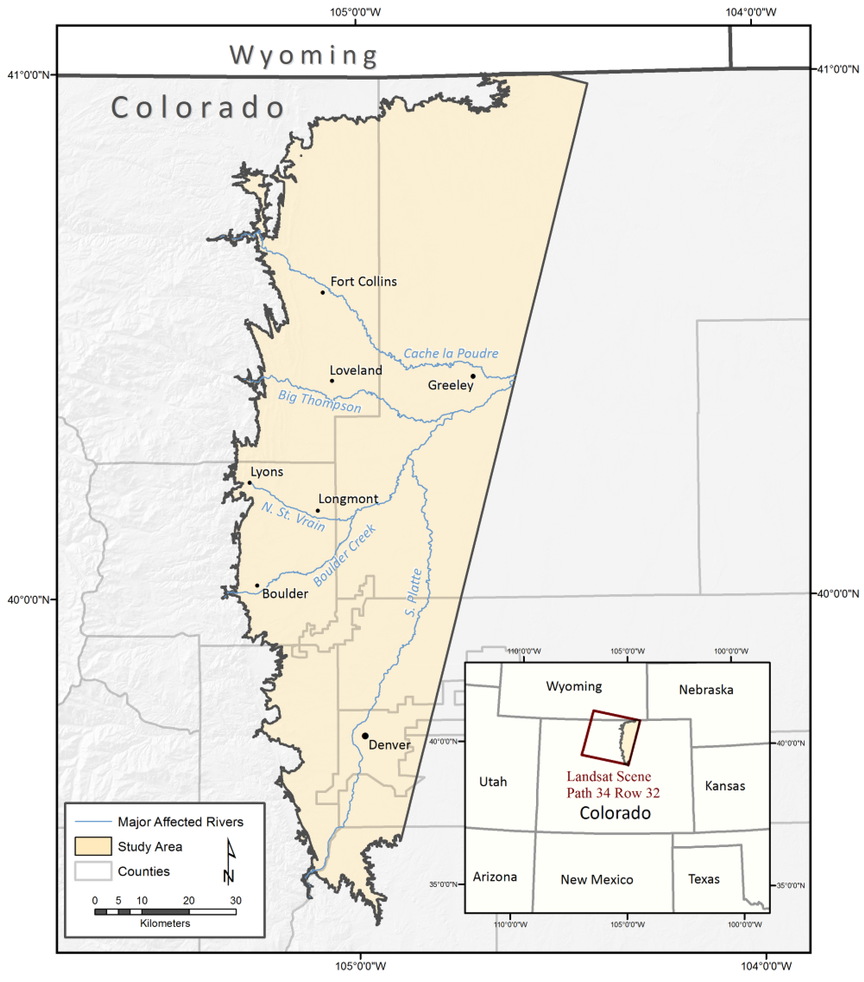
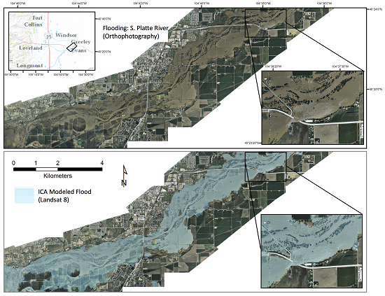
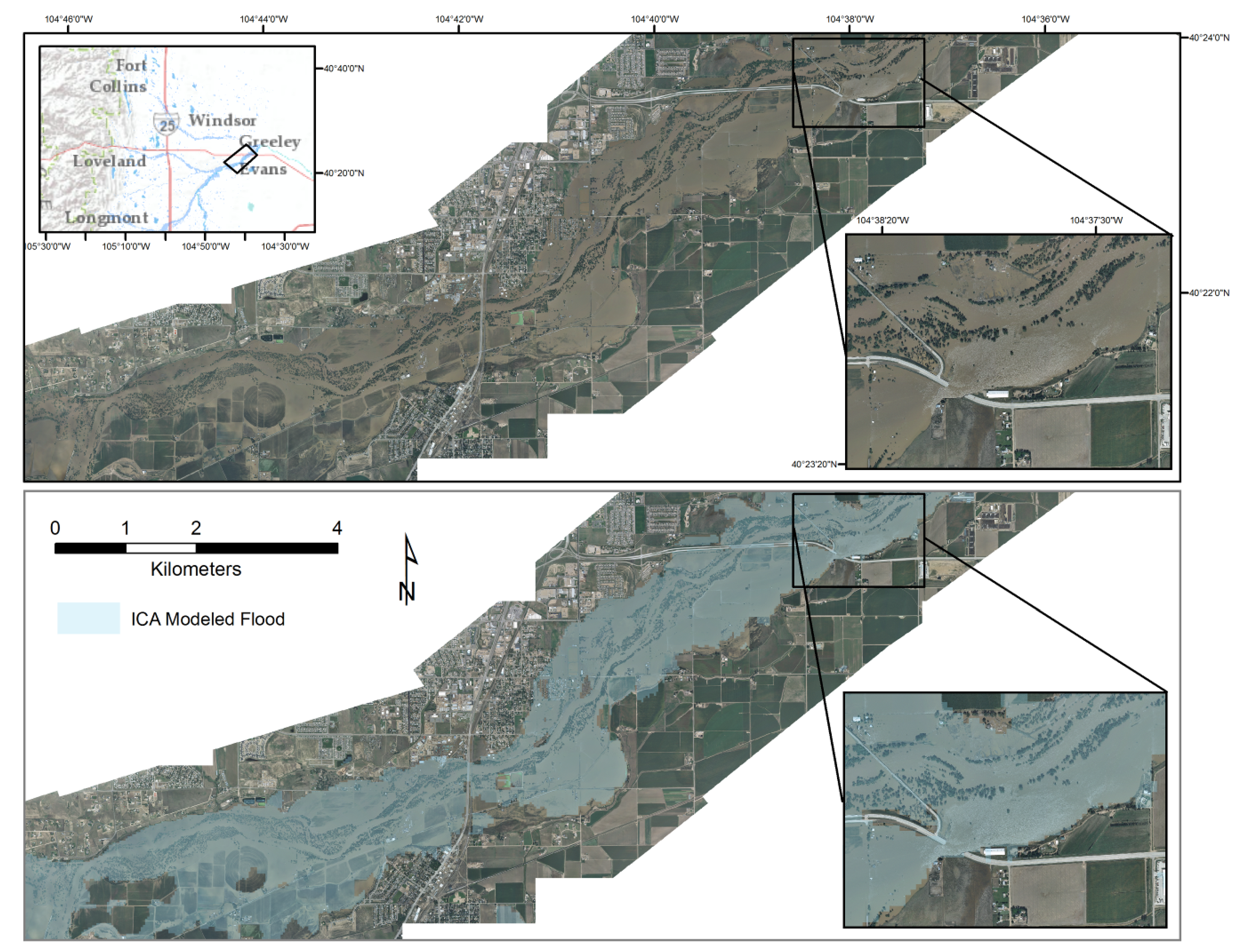
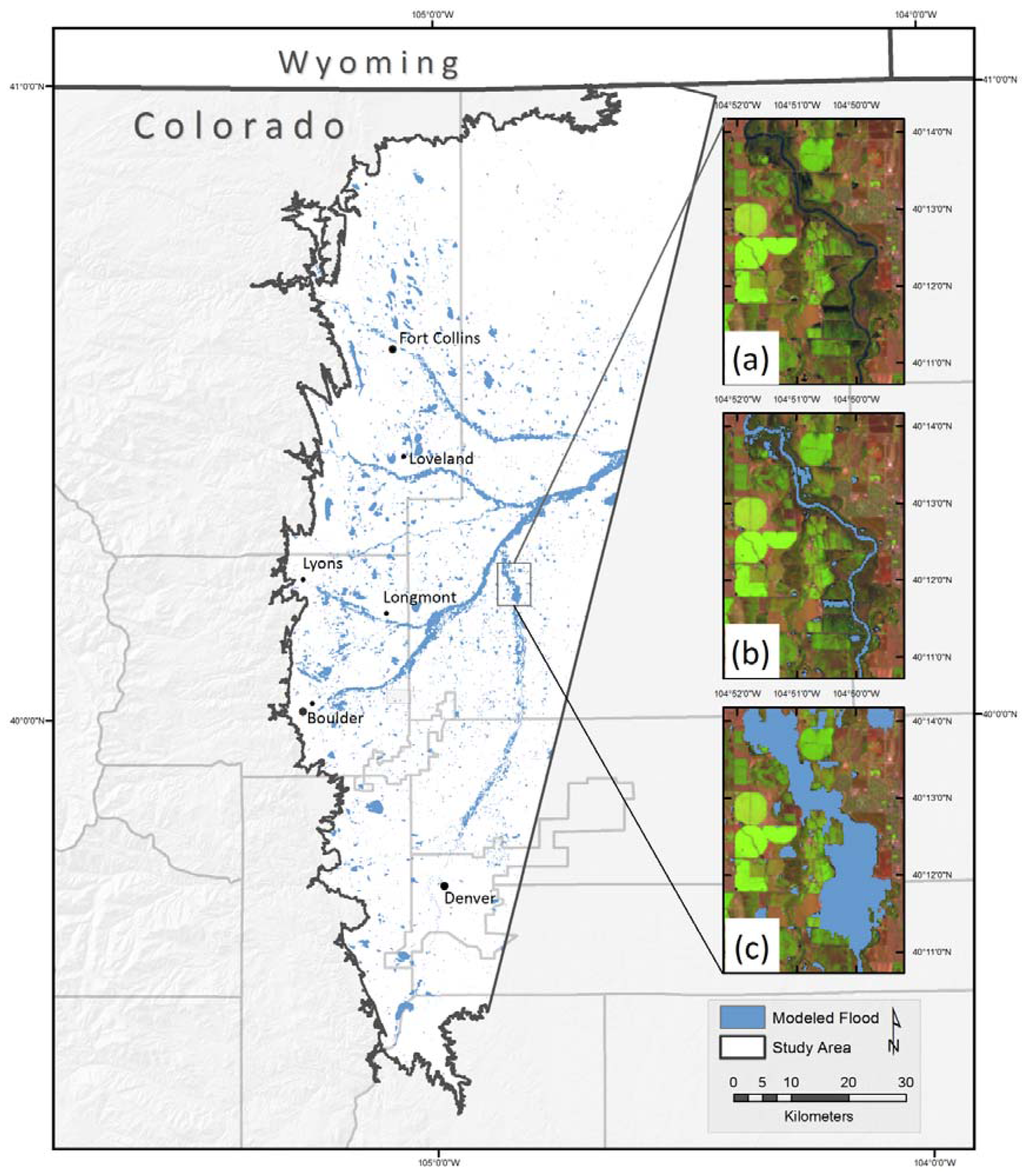
2. Study Area and Flood Event Description
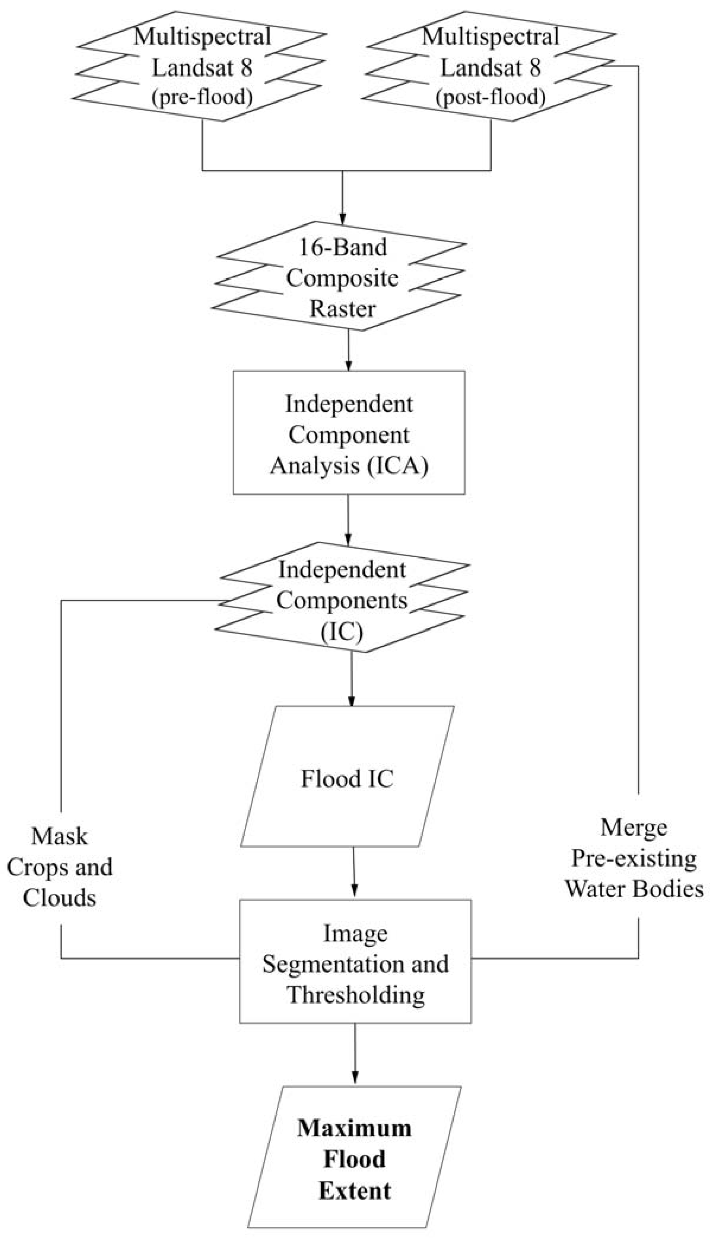
The Colorado Front Range extends north to south across the state and represents the point at which North America’s Great Plains region meets the southern Rocky Mountains. The region has long been used for irrigated agriculture, with water supplied by a number of major rivers that flow out of the steep canyons and onto the lower gradient, unconfined semi-arid high plains, which intersect the mountains at approximately 1,800 m in elevation [26]. Many of the rivers flowing west to east along the Front Range have augmented flow from transcontinental water diversions from the Colorado River Basin, pulling water from less populated to more populated regions in the state. The plains have seen a dramatic rise in population in recent decades—particularly in urban and suburban centers [27], and the region is now home to more than 80% of the Colorado population [28]. Though the typical annual peak runoff is snowmelt driven and occurs in late May and early June, extreme events have historically been generated by isolated convective thunderstorms. Elevations under 2,300 m commonly experience rainfall-induced floods that mainly occur in July and August as a result of intense, localized thunderstorms over the foothills [27].
This was the case during 9–16 September 2013, when the region experienced one of the most extreme rainfall and flooding events in Colorado recorded history. Tropical moisture drawn north from the Gulf of Mexico by a low-pressure system traveled into the Rocky Mountains and released its contents over the Front Range. Large portions of the foothills received an exceptional amount of rainfall, with 457 mm (18ʺ) falling within a period of 10 days [29]. This figure amounts to more than the annual average for the region. The majority of this precipitation fell during a period of 36 hours from September 11 to September 12 [29], with the water traveling down the system over the following days. The resulting flooding caused 250 debris slides, destruction of recreational facilities (US $44 million in damages), 615 km of destroyed roads, and US $2 billion in overall damages [30]. The event resulted in 10 human deaths and thousands of people displaced or stranded, as damage to roads and bridges cut off access to numerous residential areas. Research and assessment of this event is ongoing; while a handful of recent studies have investigated the meteorological drivers [31], peak flows and flood frequencies [29], and debris flows [32], there remains no comprehensive, regional-scale map of maximum flood extent along the high plains region.
Figure 1. Map of the Colorado Front Range and the project study site, comprised of all areas within WRS-2 Path 34, Row 32 below 1800 m in elevation. Major affected counties, cities, and rivers are included for reference.
Remotesensing 07 09822 g001
Our study focused on mapping inundation in all areas along the plains of the Front Range. The site stretches across nine counties from south of the city of Denver, Colorado to the Wyoming border (Figure 1). The base of the foothills (1800 m contour) forms the western boundary of the study site, and the eastern edge of World Reference System-2 (WRS-2) Path 34, Row 32 serves as the eastern boundary. The area contains all rivers that flow out of the mountains and join to form the main stem of the South Platte River at the eastern edge of the study site. The most prominent of these include the South Platte, Boulder Creek, Saint Vrain, Big Thompson, and Cache la Poudre Rivers.

3. Methodology

Our general workflow to map maximum flood extent was as follows (Figure 2): Pre- and post-flood multispectral Landsat 8 images were combined into a single composite raster dataset. An ICA was run on the image stack and the IC containing flooded pixels was identified. Flooded and non-flood pixels were separated using image segmentation and thresholds, and class confusion was reduced through the use of crop and cloud masks created from the other ICs. Pre-existing (unchanged) water bodies were merged with the ICA modeled flood pixels, producing a final map of maximum flood extent.
Figure 2. Workflow of the flood mapping procedure.
Remotesensing 07 09822 g002

3.1. OLI Characteristics, Data, and Processing

The Landsat 8 satellite was launched into orbit on 11 February 2013, and collects 30 m spatial resolution multispectral data at a return interval of 16 days. The increased radiometric resolution of its OLI (12-bit) instrument captures more levels of detail in each pixel than in any previous Landsat sensor. This greater quantization allows the measurement of subtle variability in surface conditions [33], which may improve the identification of residual soil moisture in areas that were inundated during a flood but dry in a post-event image. The OLI also offers significant improvements in the signal-to-noise ratio, which is estimated to reduce errors in retrieval of water characteristics to just 25% of those expected from the ETM+ sensor [33]. Furthermore, the Landsat 8 L1T product is delivered with a registration accuracy of <4.1 m across all multispectral bands, and a geometric accuracy of 7–13 m [34]; these locational improvements significantly streamline pre-processing and increase the accuracy of multi-temporal change detection [35]. The OLI is also equipped with two new bands: the “coastal/aerosol” band, which is useful for imaging shallow water, and the “cirrus” band, which is designed to identify clouds in the upper atmosphere and thus facilitate the creation of cloud masks.
When employing change detection to map flood extent, it is best to select image pairs that “book-end” the flood event as closely as possible [5,17]. We acquired two Landsat 8 images (Path 34, Row 32), the first captured 16 August 2013, and the second 17 September 2013. Both scenes were nearly cloudless within the study site, with the exception of a few clouds near the city of Boulder, Colorado in the August scene. We chose the August image to represent the pre-flood landscape, and the September image to represent the post-flood condition approximately four days after peak discharge of the region’s major rivers. These L1T terrain-corrected images were downloaded from the U.S. Geological Survey Earth Explorer (http://earthexplorer.usgs.gov/), and were radiometrically calibrated to top of atmosphere reflectance using ENVI v5.1 software. The multispectral bands from each scene served as the basis for the subsequent change detection analysis.

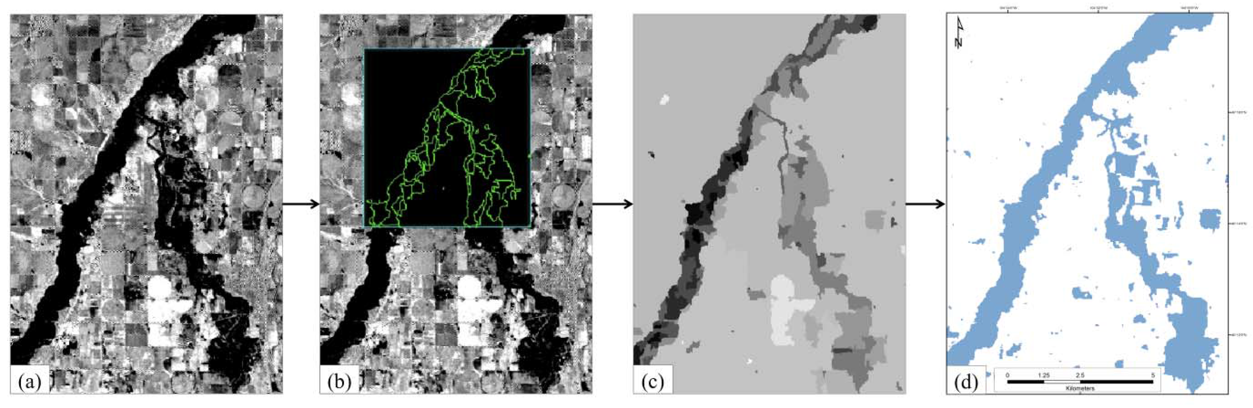
3.2. Independent Component Analysis Change Detection

The central idea of ICA is to break down a set of multivariate signals into statistically independent sources with minimal loss of information in order to achieve classification [36]. Given a set of random variables x = (x1, x2,…, xn), which are assumed to be the linear mixture of a set of statistically independent components or source signals s = (x1, x2,…, xn), the linear model of ICA is written as:
x = A s
where A is the unknown matrix of mixing parameters [19,23]. Using the given observations of x, ICA estimates A, and subsequently computes its inverse W, so that the independent components s are obtained by:
s = W x
When an ICA is applied to a raster stack of two image dates, the algorithm can accurately distinguish and categorize types of change between the two dates [18,19,37], as changed pixels are often the most uncorrelated in the dataset. Unlike the PCA, which seeks to decorrelate components in a vector, the ICA is based on higher order statistics and is thus able to identify components which may not be included in a traditional PCA [23,25]. This may have significant utility for identifying flooded areas from post-flood multispectral imagery, as moisture greatly influences reflectance values, particularly in the near infrared and shortwave infrared region of the electromagnetic spectrum [38,39]. It follows that the ICA could identify the group of pixels—or independent component—that was inundated during the flood by its distinct decrease in reflectance values.
We combined the eight multispectral bands from each Landsat scene to create a 16-band composite raster, and subsequently applied an ICA transformation to the entire image stack. Increasing the complexity of the ICA can yield more optimal signal separation, and we therefore experimented with adjusting the primary ICA parameters. This included incremental increases in the number of iterations, as well as varying the change threshold by orders of magnitude. We found that altering parameters added significant processing time to the analysis, but did not appear to produce notable changes in the resulting ICs. We therefore settled on the following parameter settings, selected for their ability to balance computational power with processing time [40]: Change Threshold = 0.0001; Maximum Iterations = 100; Maximum Stabilization Iterations = 100; Contrast Function = LogCosh (Coefficient = 1.0).
The transformation produced 16 new bands, each representing an independent component of the original composite raster. We examined each IC to determine which image class it contained, and categorized them into those that: (a) experienced change between the two dates (i.e., harvested fields, irrigated crops); (b) remained unchanged (i.e., roads, rooftops); or (c) represented image noise (haze, sensor error). The group of pixels that changed from non-water to water (i.e., flooded areas) was identified in IC band 3 (IC3). It is important to note that this IC also included pixels that were non-water in the post-flood image, but showed significant decrease in reflectance of the NIR and SWIR bands due to residual soil moisture (Figure 3a).
Following the examination of IC3, we applied standard image segmentation techniques to the band in order to separate flooded pixels from non-flooded pixels. Image segmentation partitions an image into groups of connected pixels with similar values [17,41], and we used the Extract Segments Only workflow in ENVI to accomplish this. First, we applied an edge algorithm to group neighboring pixels into objects with similar textural properties; the following parameters were used: Scale value = 80; Merge value = 0; Texture kernel size = 3. The high scale value closely delineated the inundated channel while avoiding over-segmentation, and the small kernel size prevented narrower river channels and subtle variations in the flood boundary from being lost due to generalization. A merge value of 0 was chosen in order to preserve flood objects with lower IC change values (i.e., moist soil), as their lower contrast would have otherwise resulted in their merging with neighboring dry land (Figure 3b). This process segmented the image into objects, each with a single value determined by the mean of the IC3 values of its pixels (Figure 3c). We then used the water and moisture patterns visible on the false color pre- and post-flood imagery to guide the selection of a “flooded” class threshold (in this case, a mean IC3 value ≤ 12.2).

3.3. Addition of Existing Water Bodies

Because the flood layer extracted from IC3 comprised only pixels that experienced change due to inundation, the region’s pre-existing river channels and lakes were not present in the initial flood layer. In order to include these (water-to-water) areas and delineate maximum extent, we derived the Modified Normalized Difference Water Index (MNDWI) [42] from the pre-flood image using Equation (3):
M N D W I = G r e e n S W I R 1 G r e e n + S W I R 1
where Green is the Landsat 8 band with a spectral range of 0.53–0.59 μm, and SWIR1 is the Landsat 8 shortwave infrared band with a range of 1.57–1.65 μm. The MNDWI is a commonly used index for extracting surface water [8,42,43], and is specifically designed for use in developed landscapes. The index results in values of −1 to 1, with values greater than 0 understood to represent water bodies [15]. However, manual calibration most often leads to more accurate results when applying thresholds to water indices [44], and we found pixels with MNDWI ≥ 0.15 to best represent surface water in the pre-flood Landsat 8 image. We then merged these pixels with the ICA-derived surface (Figure 3d).
Figure 3. General steps of the segmentation procedure used to extract flood features from IC3. The confluence of the Saint Vrain and South Platte Rivers is shown as an example. (a) IC3 change values shown in gray scale. (b) Flooded pixels isolated with edge filter. (c) Segmented image objects (d) Extracted ICA flood layer, merged with pre-existing water-to-water pixels (i.e., river channels and lakes).
Remotesensing 07 09822 g003

3.4. Crop and Cloud Masking

The majority of the agricultural land along the Front Range is irrigated, and we found that some of these areas were included in IC3 due to their spectral changes in moisture and greenness. This issue was largely overcome with IC9 and IC16 however, which we found to contain crops that experienced change between the image dates. These were readily identifiable by their distinctive circular (i.e., center-pivot irrigation) or rectangular shape, and their similar changes in reflectance between the pre- and post-flood Landsat scenes. We extracted these pixels using a pair of density slices (IC9 −89.8 to 2.1; IC16 −64.3 to −2.2) and merged them to create a single layer representing changed crops across the study site (total area of 192.6 km2).
To assess the fidelity of this layer, we visually compared it against high-resolution R-G-B imagery available in ESRI ArcMap software, finding close agreement with irrigated agricultural plots visible on the landscape. Additionally, we quantitatively tested its accuracy against the most current (2010) publicly available spatial data of irrigated land for the region, acquired from the state of Colorado’s Decision Support Systems website (http://cdss.state.co.us/GIS/Pages/Division1SouthPlatte.aspx). The results of an overlay analysis revealed a tight match between the two layers, with 192,197 of the 213,980 (90%) of the ICA-derived crop pixels falling within polygons of known irrigated lands.
Additionally, because we included the cirrus bands (OLI Band 9) of both Landsat 8 scenes in the original image stack, the ICA transformation was able to isolate and group all cloudy pixels into a single independent component (IC10). We again used a pair of density slices (IC10 −696.8 to −4.0; IC10 6.9 to 1739.9) to extract these pixels from the IC, using the individual cirrus bands as a visual guide for threshold selection. We then compared this layer against the Quality Assessment (QA) bands provided with all Landsat 8 L1T data, which showed the ICA-derived mask in close agreement with cloud pixels identified by the quality assessment band (QA values > 53,000). We also found the ICA cloud mask to be far superior to the QA bands for capturing cirrus clouds and avoiding confusion in bright urban areas. Following these assessments, we merged the ICA-derived cloud and crop data to create a comprehensive mask for the flood extent layer. These refinement steps resulted in a final layer representing the maximum inundation extent of the 2013 event (hereafter referred to as the “ICA modeled flood”).

4. Results and Validation
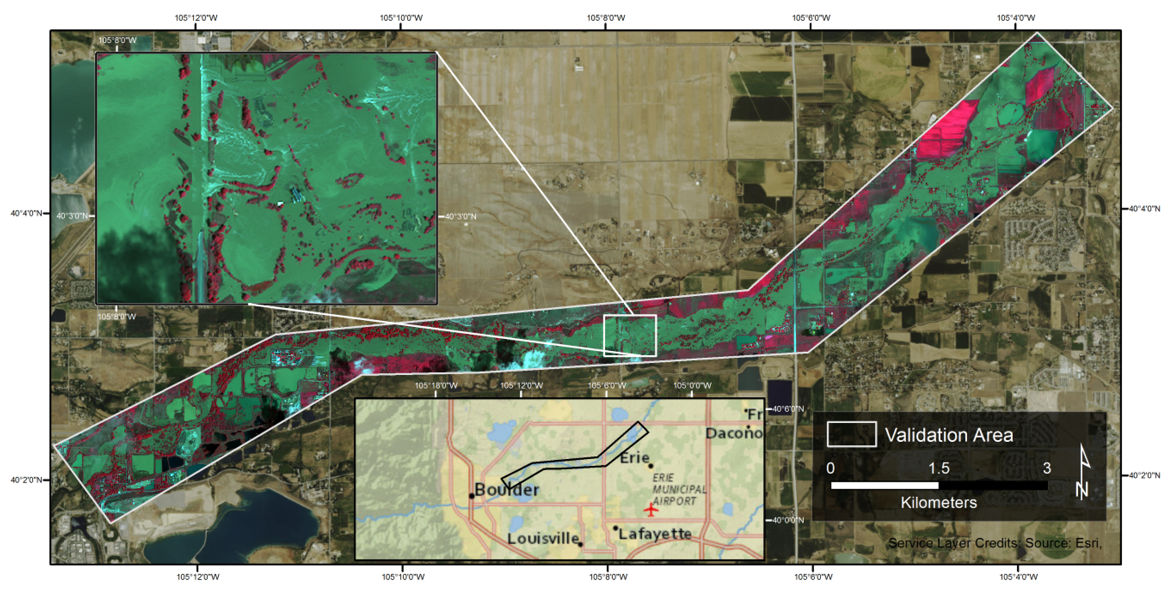
The ICA modeled flood consisted of a total area of 380 km2 across the high plains of the Colorado Front Range. An overlay analysis with the 2011 National Land Cover Dataset [45] revealed a variety of flood characteristics and impacted land cover types. First, the region’s pre-existing water bodies (NLCD class “open water”) comprised 139 km2 (37%) of the total ICA modeled flood extent. The remaining 241 km2 thus represented all areas that were inundated (non-water to water) during the 2013 event. Of these, agricultural lands were the most heavily affected cover type, with a total area of 122 km2. Wetlands and developed regions also experienced significant impacts, with inundated areas of 52 km2 and 33 km2, respectively. The remaining flood area was split between shrub/herbaceous vegetation (24 km2), forested (4 km2), and barren land (5 km2). The ICA modeled flood layer and study boundary—as well as a summary table and spatial results of affected land covers—can be found in the supplementary materials to this article (Data S1, Data S2, Data S3, Data S4, Data S5).

4.1. Validation

We used two methods, one qualitative and one quantitative, to validate the ICA modeled flood layer. First, we conducted a visual assessment against high-resolution aerial orthophotography flown on the Big Thompson, Cache la Poudre, and South Platte Rivers during the event. This was followed by a pixel-to-pixel validation with WorldView-2 (WV-2) imagery of Boulder Creek near peak flow. We then directly compared the ICA modeled flood with the post-flood MNDWI extent using a McNemar test.

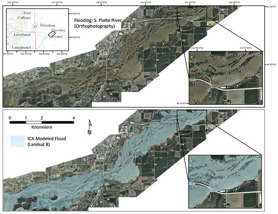
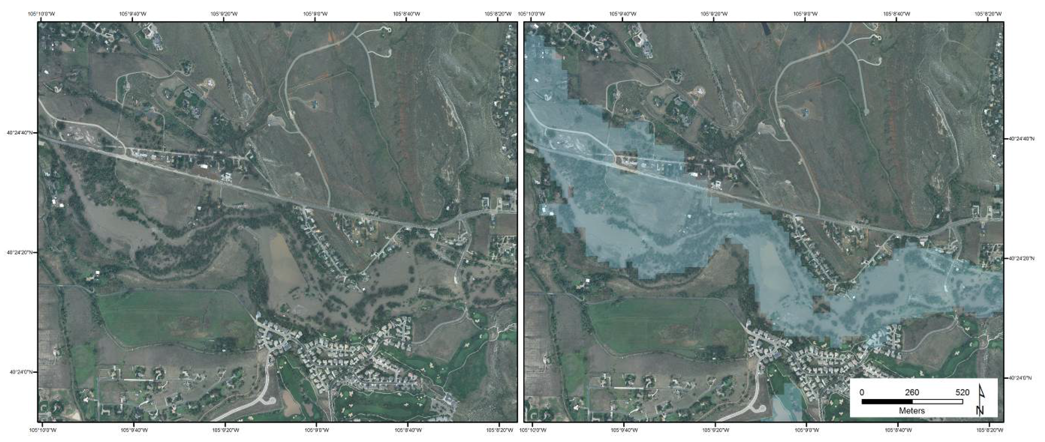
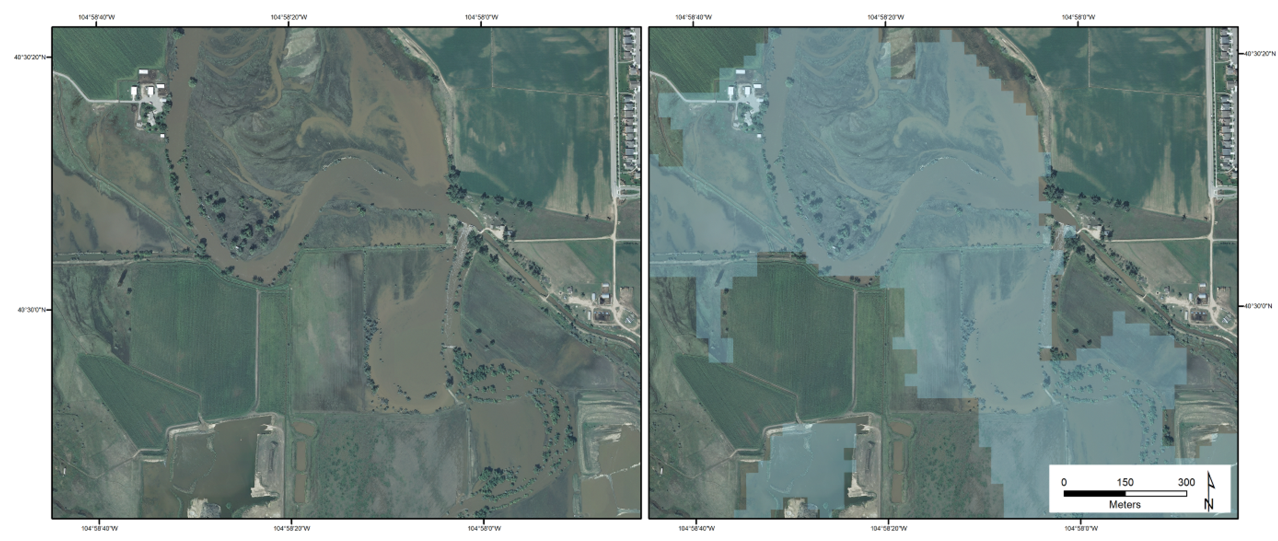
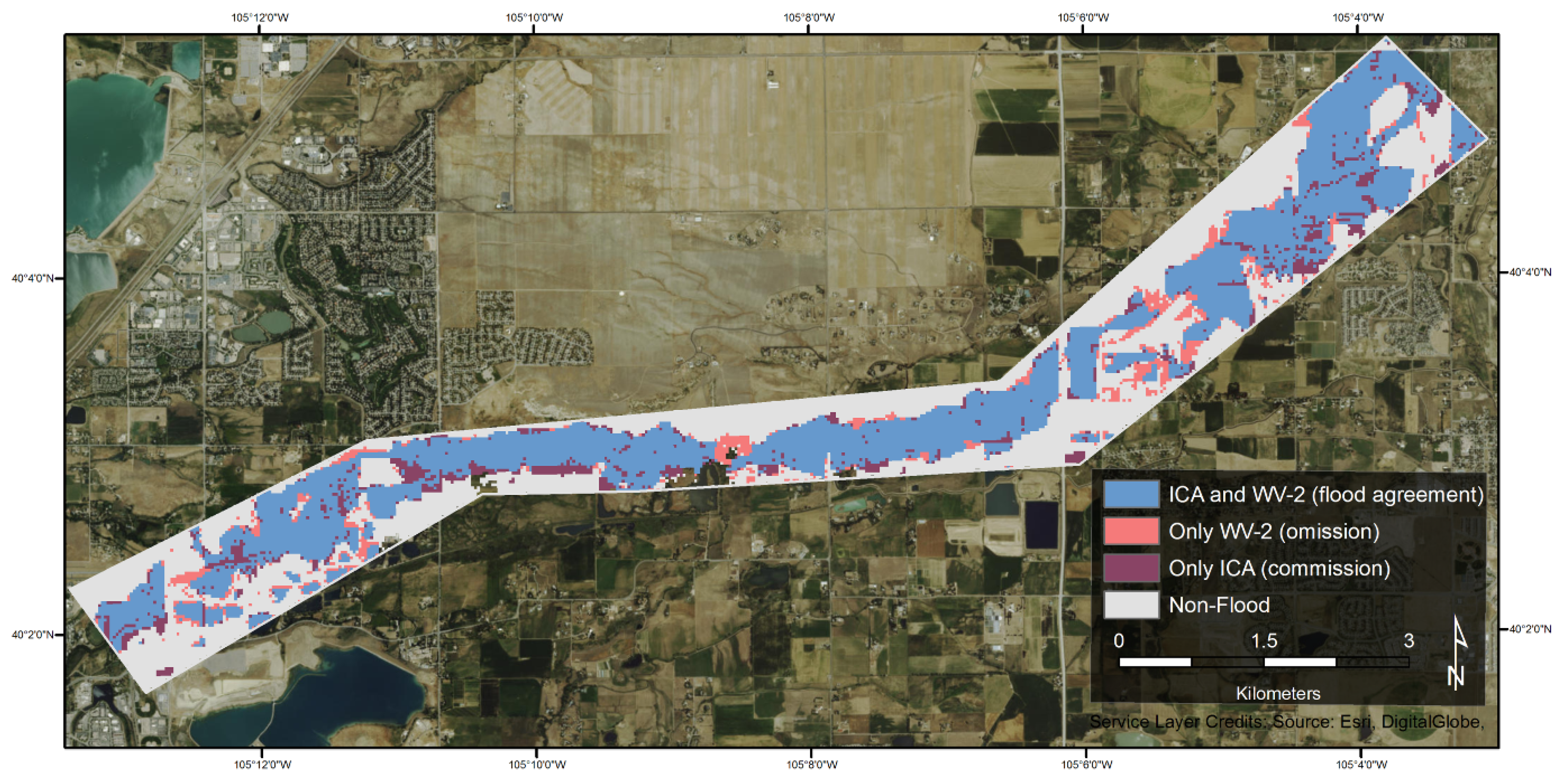
4.1.1. Visual Validation

A set of high-resolution (30 cm) R-G-B aerial orthophotographs was captured on 14 September 2013, the day when many downstream gages recorded peak flow for the 2013 event. The flight lines had a swath width of approximately 4 km, and followed the South Platte River from the Weld/Adams county line downstream to the eastern edge of the study site, as well as the Cache la Poudre and Big Thompson Rivers from their canyon mouths to their confluences with the South Platte River (Figure 4).
Figure 4. (Top) Orthophotographs of the South Platte River near Evans, Colorado. The main river channel is visible near the center of the floodplain, which is heavily inundated with floodwater (light brown). Residual moisture and pools of water can be seen near the center-pivot crop circle in the lower left corner. (Bottom) The ICA modeled flood layer overlaying the aerial imagery from the top image. Insets show detailed view of water and sediment flowing over U.S. Route 34.
Remotesensing 07 09822 g004
Visual assessment of the ICA modeled flood showed close agreement—not only with existing floodwaters—but also with scoured banks and wet soil visible in the orthophotographs (Figure 5). The comparison also revealed that the ICA successfully identified flooded areas under partial riparian canopy (Figure 6).

4.1.2. Pixel-to-Pixel Validation

Boulder Creek experienced the most extreme discharges during the 2013 flood event, peaking at 146 m3/s (5179 cfs)—nearly 20,000% above average flow [46]. While most of the Front Range was heavily clouded throughout the duration of the flood, the WV-2 satellite captured a nearly cloudless image of a reach of Boulder Creek at 18:28 on 13 September 2013 (Figure 7). This was approximately 12 hours after peak flow of Boulder Creek (which occurred the previous night), when stage height was 0.38 m (15ʺ) below the river’s maximum recorded stage during the 2013 event [46].
Figure 5. Orthophotograph of a reach of the Cache la Poudre River in Fort Collins, Colorado. The left image shows the flooding as of 14 September 2013, and the right shows the same image overlaid with the ICA modeled flood (semi-transparent blue). The flood layer closely agrees with turbid, inundated areas as well as adjacent banks scoured during the peak of the flooding.
Remotesensing 07 09822 g005
Figure 6. Orthophotograph of a reach of the Big Thompson River in Loveland, Colorado. The left image shows the flooding as of 14 September 2013, and the right shows the same image overlaid with the ICA modeled flood (semi-transparent blue).
Remotesensing 07 09822 g006
We used the cloudless section of this reach to quantitatively validate the ICA modeled results. The reference reach runs from the eastern edge of the city of Boulder, Colorado until Highway 52 near Gooding, Colorado. The area is approximately 15.5 km long and 1 km wide, and contains a variety of land uses and cover types representative of the Front Range, including developed floodplain, managed wetlands, irrigated agriculture, and riparian trees and shrubs.
Figure 7. WorldView-2 image of Boulder Creek near peak flow of the 2013 event. The image is displayed in standard false color (NIR-R-G); within the validation area, water is blue-green or black, and vegetation is red. Inset shows flooding over roads as well as the inundated floodplain.
Remotesensing 07 09822 g007
Binary pixel-to-pixel validation is a widely used approach for quantitatively assessing flood extent maps [7,14]. Reference and modeled maps are overlaid and compared on a cell-by-cell basis, resulting in a confusion matrix reporting pixels in agreement (flooded or non-flooded), as well as underprediction and overprediction.
In order to create a reference layer of maximum flood extent, we performed image segmentation on the WV-2 image to classify flooded and non-flooded regions. Additionally, we created a mask for the few cloudy areas in the south-central part of the scene, and excluded these pixels from the accuracy assessment. The WV-2 flood map was then resampled (nearest neighbor) to match the spatial resolution of Landsat 8, and the two flood layers were overlaid for the pixel-to-pixel comparison.
The validation along Boulder Creek (Figure 8) showed close agreement between the reference WV-2 layer and the ICA modeled flood, with an overall accuracy of 87%, and a Kappa Coefficient of 0.73 (Table 1). Commission errors were 12% for flooded classes and 15% for non-flooded classes. Omission errors were 15% for flooded classes and 12 % for non-flooded classes.
Additionally, in order to provide a comparison of our approach with other common flood mapping techniques, we conducted an identical pixel-to-pixel validation against the Boulder Creek reference layer using the flood extent produced from a post-flood MNDWI threshold. This resulted in an overall accuracy of 69% and a flood class accuracy of 43% (Table 2). A McNemar test comparing these results with those of the ICA modeled flood showed the latter to be significantly (p < 0.001) more accurate than the MNDWI for mapping maximum flood extent (Table 3).
Figure 8. Map of Boulder Creek showing the results of the pixel-to-pixel comparison between the ICA modeled flood and the WV-2 reference layer. Pixels in agreement, errors of omission, and errors of commission are shown in contrasting colors.
Remotesensing 07 09822 g008
Table 1. Error matrix of the pixel-to-pixel validation between the ICA and WV-2 reference layer.
Reference (WorldView-2)
ICAFloodedNon-FloodedTotal Producer’s Accuracy (%)
Flooded822113959616 85
Non-Flooded107977728851 88
Total9300916718467
User’s Accuracy (%)8885
Overall Accuracy (%)87
Kappa Coefficient0.73
Table 2. Error matrix of the pixel-to-pixel validation between the post-flood Modified Normalized Difference Water Index (MNDWI) and the WV-2 reference layer.
Reference (WorldView-2)
MNDWIFloodedNon-FloodedTotal Producer’s Accuracy (%)
Flooded41451794324 96
Non-Flooded5534860914143 61
Total9679878818467
User’s Accuracy (%)4398
Overall Accuracy (%)69
Kappa Coefficient0.40
Table 3. Results of McNemar test between ICA and post-MNDWI.
ICA CorrectICA IncorrectTotal
MNDWI Correct40291164145
MNDWI Incorrect401613815397
Total804514979542
Figure 9. Study area showing the full extent of the ICA modeled flood. Insets show a reach of the South Platte River; (a) post-flood Landsat 8 image displayed in false color (SWIR1-NIR-R): water is dark blue, moist soil is dark brown, vegetation is green, and bare ground is red-orange; (b) modeled flood extent derived from MNDWI threshold of the post-flood image: the swollen channel and other surface water is displayed in blue (c) ICA modeled flood at the same location, showing inundation of the floodplain and agreement with the dark moisture patterns visible in (a).
Remotesensing 07 09822 g009
The ICA modeled flood layer is shown in full in Figure 9, along with a visual comparison of the MNDWI and ICA extents. The ICA modeled flood constitutes 58% more flooded area than the MNDWI threshold of the post-flood image (222 km2), indicating that the approach not only captured the open water visible in the scene, but also residual moisture (Figure 9a–c).

5. Discussion

5.1. Strengths and Advantages

Our analysis was able to simultaneously delineate flood-related surface water and soil in very narrow channels—some only two or three Landsat pixels in width—across multiple drainages and surrounding land cover types. Moreover, this was accomplished without the use of clumping procedures and moving windows that are often applied to smooth flood width maps [17,47,48]. While such post-processing techniques can be appropriate for large river systems with deep, homogenous channels, they yield layers that homogenize the channel variability observed in more shallow, braided rivers—one of the most important yet difficult aspects of a flood to capture with stream gages [3].
The multi-temporal ICA approach also provides flexibility to the analyst; if only inundated pixels (i.e., non-water to water) are all that is required, the ICA accurately and automatically provides this through its identification of change classes. However, if existing channels and water bodies (i.e., water to water) are also needed, these can be merged with the flood layer using a water index threshold from the pre-flood image, as was done in this study.
The ability of the ICA to separate non-flood change classes such as agriculture proved extremely useful for refining the flood layer in a heavily irrigated landscape like the high plains of the Front Range. This is a robust and valuable asset that enables more accurate assessment of flood impacts in developed and cultivated floodplains. The ICA also produced an excellent cloud mask; although our images were nearly cloudless in the study site, this ability could be very useful in streamlining data processing for future studies employing imagery with greater proportions of cloud cover. This also demonstrates the benefit of including the multispectral cirrus bands as an integral part of the change analysis.
An additional strength of the approach is the consistent time period and spatial scale of its results. This enables the comparison of flood impacts across municipal and hydrologic boundaries, facilitates targeting of field measurements, and promotes cross-basin management and recovery decisions in a way not possible with localized mapping efforts. This has powerful implications when considered with the free and global coverage of Landsat data and the availability of ICA code through ENVI, MatLab, R, and Python. Finally, the relatively straightforward nature of the procedure—and its independence from ancillary training data or elevation models—makes it accessible and applicable for a wide variety of users and settings.

5.2. Errors and Limitations

The errors observed in this study are the result of a number of factors. The floodplains and channel margins of the Great Plains streams host numerous gallery cottonwood (Populus deltoides) forests. While many flooded areas beneath moderate or sparse riparian canopy were accurately identified by our analysis, pixels with dense or complete canopy cover were not captured. This contributes to the overall omission error, as the consistent vegetation crown prevents the identification of change between pre- and post-flood images—even if the ground at the base of the tree and was inundated during the event. Omission errors also occurred in paved areas and along concrete channel banks, as their impermeability and ability to move floodwater through the system prevent large changes in moisture.
Although most of the irrigated crops misclassified as flooded were identified and masked using the other ICs, some experienced a change in spectral values so similar to flooding between dates that they were still present in the final flood layer. While we focused on a strictly remote sensing approach, the majority of these erroneous areas could be removed as needed in post-processing through expert interpretation of the results with ancillary geospatial layers and field observations. For instance, “flooded” areas that form clear geometric shapes (i.e., crop circles) and are isolated from the river channel could be manually removed with a high degree of confidence.
Another consideration is the 30 m spatial resolution of Landsat 8. The cell size likely contributed to confusion in developed areas, where floodwaters move between homes, vehicles, and other urban features. This increases the brightness of otherwise dark pixels, resulting in higher numbers of omission errors. The resolution also makes precise delineation of the flood edge difficult at the scale necessary for detailed assessment of geomorphic change. It is also important to note that our study benefited from the availability of a post-flood image captured only days after the most extreme flooding, when many inundated areas were still saturated at the surface. This reinforces the importance of using imagery as close to the event as possible, as the detectability of such changes will decrease as the moisture conditions of the surface return to their normal state. While residually wet soils and stressed vegetation can be observed from one to two weeks after a flood [49,50], the window of time for mapping these with an ICA change detection will likely vary with the magnitude of the event, the soil properties of the study area, and the sensor being employed. The method may also have challenges in steep topography or canyons, where floodplains are narrower and flooding occurs more in the vertical (i.e., river stage) than the horizontal (i.e., lateral extent across the floodplain) direction.

5.3. Future Work

The response to the damages to human infrastructure that occurred in the 2013 Colorado event has resulted in the reconstruction of roads and stream crossings, as well as simplification, straightening, and—and in some cases—narrowing of stream channels. Flood recovery efforts that result in streams engineered to convey floods as efficiently as possible through simplified channels are in direct conflict of managing streams for natural channel processes, productive fisheries, and other valuable ecosystem services. The spatial data produced from this study can be used for comparisons of flood impacts across multiple catchments, as well as inform management decisions and guide research on the function of extreme floods in ecohydrological processes that maintain dynamic, productive and diverse riparian habitats [51]. These data can also be used for flood hazard and flood risk mapping to aid in the establishment of flood warning systems. Where available, high-resolution digital elevation models can be used in conjunction with the measure of flood width to estimate a number of hydrologic parameters including flood depth, velocity, stream power and shear stress.
Many of the challenges we encountered may be overcome through application of the ICA with imagery from the upcoming Sentinel-2 satellite pair (European Space Agency). The multispectral instrument onboard the satellites will feature relatively high spatial resolution in both the Visible to NIR (10 m) and Red Edge to SWIR (20 m) regions of the electromagnetic spectrum [33], which will enable finer delineation of the flood edge. Moreover, the Sentinel-2 program has been cross-calibrated for integration with Landsat 8 data [33], will have a revisit time of 1–4 days (depending on latitude) [52], and is planned to share the latter’s free and open data policy [53]. This will significantly increase the availability of comparable imagery that bookend flood events, and is an exciting avenue for future research.

6. Conclusions

This study explored the utility of Landsat 8 multispectral data and independent component analysis for delineating maximum flood extent through an unsupervised change detection procedure. The analysis was conducted across multiple catchments possessing narrow channels and heavily developed floodplains in the high plains of the Colorado Front Range. Results were qualitatively and quantitatively assessed against multiple reference data, and subsequently compared with a modified difference water index commonly used to map floods in developed landscapes.
Our results produced a consistent, regional-scale flood layer with an overall accuracy of 87%, and close agreement with high-resolution aerial orthophotographs captured near peak flow. The spatial data of flood extent was provided for ongoing hydrologic and mitigation planning in the region, and showed a maximum flood area of 380 km2 across a variety of land cover types. Excluding pre-existing water bodies, a total of 241 km2 was inundated in the event, with agricultural land comprising the largest impacted area (122 km2).
Our study also revealed a number of important characteristics of the OLI-based independent component analysis for flood mapping. The ability of the ICA change detection to identify residually wet soils inundated during peak flow resulted in it being 44% more accurate for mapping maximum flood extent than the standard MNDWI-based technique. Moreover, because these results were achieved without the use of post-processing smoothing operations, they retained the spatial variability of flooding within the complex and braided channels of the study site. This an important—yet rarely captured—flood characteristic that is critical for understanding the nuanced patterns of floods, particularly in heavily managed and engineered river systems. Although flooded pixels under dense vegetation cover caused omission errors, flooded areas under moderate or sparse riparian canopy were accurately classified. We also found the approach to be effective for identifying subtle class differences in the images; this provided useful data with which to mask irrigated agriculture that experienced spectral changes similar to flooding, and may significantly help to refine flood maps in other developed and heterogeneous floodplains.
These findings offer change detection with OLI and ICA to be a powerful tool for overcoming some of the long-standing issues in optical remote sensing of flood mapping. The procedure is both robust and flexible, as it can be applied to capture only inundated pixels, or combined with pre-existing water features to map maximum extent. The method also has significant potential for consistent and international application, as it requires no ancillary training data or elevation models, making it highly applicable in remote regions where Landsat imagery is all that is available. While the temporal and spatial resolutions of Landsat 8 remain challenges in certain settings, these may be significantly reduced through cross-calibration and integration with upcoming satellites and multispectral sensors. This—in combination with field measurements and expert opinion—could rapidly produce maps for emergency responders and hydrologists to focus rescue and remediation efforts, and the consistent time period, spatial scale, and method of creation facilitate the comparison and management of flood impacts across municipal and hydrologic boundaries.

Acknowledgments

This study was conducted at the Natural Resource Ecology Laboratory and the Geospatial Centroid at Colorado State University. The material is based upon work supported by NASA under award No. NNX14AB60A. Additional support was provided by the US Geological Survey. The authors thank four anonymous reviewers whose feedback considerably added to the quality of the final manuscript. Recognition and thanks are also due to previous NASA DEVELOP team members Sky Skach and Amber Weimer who contributed to the early stages of this project. Special thanks to Stephen Leisz, Sophia Linn, Steven Yochum, and Nicholas Young for their support and feedback. The authors also gratefully acknowledge the Colorado Water Conservation Board and Colorado Department of Natural Resources for facilitating access to the aerial orthophotography.

Author Contributions

Stephen Chignell, Ryan Anderson, Melinda Laituri, and Paul Evangelista conceived and designed the study. Stephen Chignell and Ryan Anderson performed the analyses and wrote the manuscript. David Merritt led the visual validation and guided interpretation of the results. All authors provided feedback and text to significantly improve the quality of the final manuscript.

Supplementary Information

Data S1: Maximum_Inundation_Extent.kmz, Data S2: Maximum_Inundation_Extent.tif, Data S3: Study_Area.shp, Data S4: Inundated_Land_Cover_Summary, Data S5: Inundated_Land_Cover.tif.

Conflicts of Interest

The authors declare no conflict of interest.

References

  1. Bates, B.C.; Kundzewicz, Z.W.W.; Wu, S.; Palutikof, J.P. Linking Climate Change and Water Resources: Impacts and Responses; IPCC Secretariat: Geneva, Switzerland, 2008. [Google Scholar]
  2. Stocker, T.F.; Qin, D.; Plattner, G.-K.; Tignor, M.; Allen, S.K.; Boschung, J.; Nauels, A.; Xia, Y.; Bex, V.; Midgley, P.M. Climate Change 2013: The Physical Science Basis. Contribution of Working Group I to the Fifth Assessment Report of the Intergovernmental Panel on Climate Change; AR5; IPCC: Geneva, Switzerland, 2013. [Google Scholar]
  3. Alsdorf, D.E.; Rodriquez, E.; Lettenmaier, D.P. Measuring surface water from space. Rev. Geophys. 2007, 45, 1–24. [Google Scholar] [CrossRef]
  4. Boori, M.S.; Voženílek, V. Remote sensing and GIS for socio-hydrological vulnerability. J. Geol. Geosci. 2014, 3, 1–4. [Google Scholar]
  5. Wang, Y. Mapping extent of floods: What we have learned and how we can do better. Nat. Hazards Rev. 2002, 3, 68–73. [Google Scholar] [CrossRef]
  6. Smith, L. Satellite remote sensing of river inundation area, stage, and discharge: A review. Hydrol. Process. 1997, 11, 1427–1439. [Google Scholar] [CrossRef]
  7. Schumann, G.; Bates, P.D.; Horritt, M.S.; Matgen, P.; Pappenberger, F. Progress in integration of remote sensing-derived flood extent and stage data and hydraulic models. Rev. Geophys. 2009, 47, 1–21. [Google Scholar] [CrossRef]
  8. Zhang, R.; Sun, Y. Rapid extraction of Pakistan floods from TM images. In Proceedings of the IEEE 2012 20th International Conference on Geoinformatics, Hong Kong, China, 15–17 June 2012; pp. 1–4.
  9. Amarnath, G. An algorithm for rapid flood inundation mapping from optical data using a reflectance differencing technique. J. Flood Risk Manag. 2013, 7, 239–250. [Google Scholar] [CrossRef]
  10. Ticehurst, C.; Guerschman, J.P.; Chen, Y. The strengths and limitations in using the Daily MODIS Open Water Likelihood Algorithm for identifying flood events. Remote Sens. 2014, 6, 11791–11809. [Google Scholar] [CrossRef]
  11. Opolot, E. Application of remote sensing and Geographical Information Systems in flood management: A review. Res. J. Appl. Sci. Eg. Technol. 2013, 6, 1884–1894. [Google Scholar]
  12. Wang, Y. Using Landsat 7 TM data acquired days after a flood event to delineate the maximum flood extent on a coastal floodplain. Int. J. Remote Sens. 2004, 25, 959–974. [Google Scholar] [CrossRef]
  13. Islam, A.S.; Bala, S.K.; Haque, M.A. Flood inundation map of Bangladesh using MODIS time-series images. J. Flood Risk Manag. 2010, 3, 210–222. [Google Scholar] [CrossRef]
  14. Li, S.; Sun, D.; Goldberg, M.; Stefanidis, A. Derivation of 30-m-resolution water maps from TERRA/MODIS and SRTM. Remote Sens. Environ. 2013, 134, 417–430. [Google Scholar] [CrossRef]
  15. Huang, C.; Chen, Y.; Wu, J. Mapping spatio-temporal flood inundation dynamics at large river basin scale using time-series flow data and MODIS imagery. Int. J. Appl. Earth Obs. Geoinf. 2014, 26, 350–362. [Google Scholar] [CrossRef]
  16. Wang, Y.; Colby, J.D.; Mulcahy, K.A. An efficient method for mapping flood extent in a coastal floodplain using Landsat TM and DEM data. Int. J. Remote Sens. 2002, 23, 3681–3696. [Google Scholar] [CrossRef]
  17. Gianinetto, M.; Villa, P.; Lechi, G. Postflood damage evaluation using Landsat TM and ETM+ data integrated with DEM. IEEE Trans. Geosci. Remote Sens. 2006, 44, 236–243. [Google Scholar] [CrossRef]
  18. Marchesi, S.; Bruzzone, L. ICA and kernel ICA for change detection in multispectral remote sensing images. In Proceedings of the 2009 IEEE International Geoscience and Remote Sensing Symposium, Cape Town, South Africa, 12–17 July 2009; Volume 2, pp. II–980–II–983.
  19. Zhong, J.; Wang, R. Multi-temporal remote sensing change detection based on independent component analysis. Int. J. Remote Sens. 2006, 27, 2055–2061. [Google Scholar] [CrossRef]
  20. Volpi, M.; Petropoulos, G.P.; Kanevski, M. Flooding extent cartography with Landsat TM imagery and regularized kernel Fisher’s discriminant analysis. Comput. Geosci. 2013, 57, 24–31. [Google Scholar] [CrossRef]
  21. Ireland, G.; Volpi, M.; Petropoulos, G. Examining the capability of supervised machine learning classifiers in extracting flooded areas from Landsat TM imagery: A case study from a Mediterranean flood. Remote Sens. 2015, 7, 3372–3399. [Google Scholar] [CrossRef] [Green Version]
  22. Comon, P. Independent component analysis, A new concept? Sig. Process. 1994, 36, 287–314. [Google Scholar] [CrossRef] [Green Version]
  23. Hyvärinen, A.; Oja, E. Independent component analysis: Algorithms and applications. Neural Netw. 2000, 13, 411–430. [Google Scholar] [CrossRef]
  24. Zhang, X. New independent component analysis method using higher order statistics with application to remote sensing images. Opt. Eng. 2002, 41, 1717–1728. [Google Scholar] [CrossRef]
  25. Hyvärinen, A. Survey on independent component analysis. Neural Comput. Surv. 1999, 2, 94–128. [Google Scholar]
  26. Windell, J.T.; Willard, B.E.; Cooper, D.J.; Foster, S.Q.; Knud-Hansen, C.F.; Rink, L.P.; Kiladis, G.N. An Ecological Characterization of Rocky Mountain Montane and Subalpine Wetlands; Denver Wildlifre Research Center, U.S. Fish and Wildlife Service: Denver, CO, USA, 1986; Volume 86. [Google Scholar]
  27. Wohl, E.E. Virtual Rivers: Lessons from the Mountain Rivers of the Colorado Front Range; Yale University Press: New Haven, CT, USA, 2001. [Google Scholar]
  28. United States Census Bureau. United States Census 2010; Government Printing Office: Washington, DC, USA, 2012. [Google Scholar]
  29. Yochum, S.E. Colorado Front Range Flood of 2013: Peak Flows and Flood Frequencies. In Proceedings of the 3rd Joint Federal Interagency Conference on Sedimentation and Hydrologic Modeling, Reno, NV, USA, 19–23 April 2015; pp. 1–12.
  30. USDA Lessons from the 2013 northern Colorado flood: Past, present, and future. Available online: http://www.fs.fed.us/rmrs/news/releases/content/?id=14-04-22 (accessed on 10 April 2015).
  31. Gochis, D.; Schumacher, R.; Friedrich, K.; Doesken, N.; Kelsch, M.; Sun, J.; Ikeda, K.; Lindsey, D.; Wood, A.; Dolan, B.; et al. The Great Colorado Flood of September 2013. Bull. Am. Meteorol. Soc. 2014. [Google Scholar] [CrossRef]
  32. Anderson, S.W.; Anderson, S.P.; Anderson, R.S. Exhumation by debris flows in the 2013 Colorado Front Range storm. Geology 2015, 43, 1–4. [Google Scholar] [CrossRef]
  33. Roy, D.P.; Wulder, M.A.; Loveland, T.R.; Woodcock, C.E.; Allen, R.G.; Anderson, M.C.; Helder, D.; Irons, J.R.; Johnson, D.M.; Kennedy, R.; et al. Landsat-8: Science and product vision for terrestrial global change research. Remote Sens. Environ. 2014, 145, 154–172. [Google Scholar] [CrossRef]
  34. Storey, J.; Choate, M.; Lee, K. Landsat 8 Operational Land Imager on-orbit geometric calibration and performance. Remote Sens. 2014, 6, 11127–11152. [Google Scholar] [CrossRef]
  35. Townshend, J.R.G.; Justice, C.O.; Gurney, C.; McManus, J. The impact of misregistration on change detection. IEEE Trans. Geosci. Remote Sens. 1992, 30, 1054–1060. [Google Scholar] [CrossRef]
  36. Du, Q.; Kopriva, I.; Szu, H. Independent Component Analysis for classifying multispectral images with dimensionality limitation. Int. J. Inf. Acquis. 2004, 1, 201–216. [Google Scholar] [CrossRef]
  37. Ceccarelli, M.; Petrosino, A. Unsupervised change detection in multispectral images based on Independent Component Analysis. In Proceedings of the International Workshop on Imaging System and Techniques, Minory, Italy, 29 April 2006; pp. 54–59.
  38. Lobell, D.B.; Asner, G.P. Moisture effects on soil reflectance. Soil Sci. Soc. Am. J. 2002, 66, 722–727. [Google Scholar] [CrossRef]
  39. Skidmore, E.L.; Dickerson, J.D.; Schimmelpfennig, H. Evaluating surface-soil water content by measuring reflectance. Soil Sci. Soc. Am. J. 1975, 39, 238–242. [Google Scholar] [CrossRef]
  40. ExelisVIS Independent Component Analysis. Documentation Center. Available online: http://exelisvis.com/docs/IndependentComponentsAnalysis.html (accessed on 29 January 2015).
  41. Pal, N.R.; Pal, S.K. A review on image segmentation techniques. Pattern Recognit. 1993, 26, 1277–1294. [Google Scholar] [CrossRef]
  42. Xu, H. Modification of normalised difference water index (NDWI) to enhance open water features in remotely sensed imagery. Int. J. Remote Sens. 2006, 27, 3025–3033. [Google Scholar] [CrossRef]
  43. Feyisa, G.L.; Meilby, H.; Fensholt, R.; Proud, S.R. Automated Water Extraction Index: A new technique for surface water mapping using Landsat imagery. Remote Sens. Environ. 2014, 140, 23–35. [Google Scholar] [CrossRef]
  44. Ji, L.; Zhang, L.; Wylie, B. Analysis of dynamic thresholds for the Normalized Difference Water Index. Photogramm. Eng. Remote Sens. 2009, 75, 1307–1317. [Google Scholar] [CrossRef]
  45. Homer, C.; Dewitz, J.; Yang, L.; Jin, S.; Danielson, P.; Xian, G.; Coulston, J.; Herold, N.; Wickham, J.; Megown, K. Completion of the 2011 National Land Cover Database for the conterminous United States—Representing a decade of land cover change information. Photogramm. Eng. Remote Sens. 2015, 81, 345–354. [Google Scholar]
  46. USGS National Water Information System. Available online: http://waterdata.usgs.gov/co/nwis/ (accessed on 29 January 2015).
  47. Villa, P.; Gianinetto, M. Multispectral transform and spline interpolation for mapping flood damages. In Proceedings of the 2006 IEEE International Conference on Geosceinces and Remote Sensing Symposium, Denver, CO, USA, 31 July–4 August 2006.
  48. Gianinetto, M.; Villa, P. Monsoon flooding response: A multi-scale approach to water-extent change detection. Int. Arch. Photogramm. Remote Sens. Spat. Inf. Sci. 2006, 36, 128–133. [Google Scholar]
  49. Morrison, R.; White, P. Monitoring Flood Inundation; United States Geol. Surv. Prof. Pap. 929; ERTS-1, A New Window on Our Planet; 1974; pp. 196–208. [Google Scholar]
  50. Rango, A.; Salomonson, V.V. Regional flood mapping from space. Water Resour. Res. 1974, 10, 473–484. [Google Scholar] [CrossRef]
  51. Merritt, D. Reciprocal relations between riparian vegetation, fluvial landforms, and channel processes. In Treatise on Geomorphology; Shroder, J., Wohl, E.E., Eds.; Academic Press: San Diego, CA, USA, 2013; pp. 219–243. [Google Scholar]
  52. Drusch, M.; Del Bello, U.; Carlier, S.; Colin, O.; Fernandez, V.; Gascon, F.; Hoersch, B.; Isola, C.; Laberinti, P.; Martimort, P.; et al. Sentinel-2: ESA’s Optical High-Resolution Mission for GMES Operational Services. Remote Sens. Environ. 2012, 120, 25–36. [Google Scholar] [CrossRef]
  53. Quartulli, M.; Olaizola, I.G. A review of EO image information mining. ISPRS J. Photogramm. Remote Sens. 2013, 75, 11–28. [Google Scholar] [CrossRef]

