Calibration of the L-MEB Model for Croplands in HiWATER Using PLMR Observation ^†

Abstract

The Soil Moisture and Ocean Salinity (SMOS) mission was initiated in 2009 with the goal of acquiring global soil moisture data over land using multi-angular L-band radiometric measurements. Specifically, surface soil moisture was estimated using the L-band Microwave Emission of the Biosphere (L-MEB) radiative transfer model. This study evaluated the applicability of this model to the Heihe River Basin in Northern China for specific underlying surfaces by simulating brightness temperature (BT) with the L-MEB model. To analyze the influence of a ground sampling strategy on the simulations, two resampling methods based on ground observations were compared. In the first method, the simulated BT of each point observation was initially acquired. The simulations were then resampled at a 1 km resolution. The other method was based on gridded data with a resolution of 1 km averaged from point observations, such as soil moisture, soil temperature, and soil texture. The simulated BTs at a 1 km resolution were then obtained using the L-MEB model. Because of the large variability in soil moisture, the resampling method based on gridded data was used in the simulation. The simulated BTs based on the calibrated parameters were validated using airborne L-band data from the Polarimetric L-band Multibeam Radiometer (PLMR) acquired during the HiWATER project. The root mean square errors (RMSEs) between the simulated results and the PLMR data were 6 to 7 K for V-polarization and 3 to 5 K for H-polarization at different angles. These results demonstrate that the model effectively represents agricultural land surfaces, and this study will serve as a reference for applying the L-MEB model in arid regions and for selecting a ground sampling strategy.

1. Introduction

Soil moisture is a key component between the hydrosphere, biosphere and atmospheric water cycle and significantly affects the redistribution of rainfall into infiltration, surface runoff and evaporation at the earth’s surface [1]. For a small watershed, in situ soil moisture data can be acquired through gravimetric sampling or time domain reflectometry (TDR) sensors [2]; however, data collection is time consuming when applied at a large scale. Recently, progress in remote sensing technology has provided a new approach to global soil moisture monitoring. New satellite missions, such as the Advanced Microwave Scanning Radiometer 2 (AMSR2) [2], Soil Moisture and Ocean Salinity (SMOS) [3], Soil Moisture Active Passive (SMAP) [4], and Aquarius [5], have produced soil moisture datasets. Compared with other space-borne radiometer bands, the L-band (1–2 GHz) is the most sensitive to soil moisture [6]. Additionally, microwave radiation has all-weather, all-day capabilities. Therefore, developing a soil moisture inversion algorithm for the L-band is important for monitoring the global water cycle.

In 2009, the European Space Agency launched SMOS with the goal of obtaining global soil moisture and ocean salinity estimates. The L-band Microwave Emission of the Biosphere model (L-MEB) is used as a forward model in developing a SMOS soil moisture inversion algorithm. The model considers the contributions of various underlying surface types, including bare soil, vegetation and open water, to the total radiative energy [6]. Based on the L-MEB model, Pellarin et al. [7] simulated brightness temperature (BTs) over land surfaces at a half-degree resolution globally in 2003. These authors significantly contributed to the evaluation of the sensitivity of satellite-based L-band radiometry data to soil moisture. In 2015, Li et al. [8] analyzed and reduced uncertainties in soil moisture retrieval based on the L-MEB model using L-band microwave BTs. The retrieval uncertainties in soil moisture were mainly caused by observation error, parameter uncertainty and the retrieval strategy. The soil moisture retrieval accuracy was determined using both the total sensitivity of each model parameter and the coupling effect between soil moisture and other parameters. Because the L-MEB model is a crucial component of the SMOS Level 2 (SMOS L2) algorithm, calibrating the soil and vegetation parameters of the model is important. In 2007, Wigneron et al. [9] further detailed the L-MEB model and evaluated the applicability of the model with several experimental datasets that involved agricultural crops in Avignon and Michigan. In 2008, Grant et al. [10] simulated the BTs of coniferous and deciduous forest canopies in Bordeaux and West Germany, respectively, using the L-MEB model. The authors calibrated the vegetation parameters under forest cover and verified the optical thickness relationship with the leaf area index (LAI). The results were then used in the SMOS L2 soil moisture algorithm.

To understand the relative roles of various underlying components in L-band microwave radiation, most researchers have studied the influence of land surface parameters using a large number of ground observation experiments and BT simulations [11,12,13,14]. Saleh et al. [11] simulated the BT of grasslands using the L-MEB model, established a nonlinear regression relationship between the simulation results and soil moisture, and proposed a new method for estimating the effects of vegetation and soil roughness on soil moisture retrieval. Ferrazzoli et al. [12] observed that in the process of simulating forest canopy BTs, the microwave radiation in the L-band mainly derives from the branches, whereas the effects of the trunk are smaller. Wigneron et al. [13] simulated the BTs of various crop types using the L-MEB model and adjusted the optical thickness and single-scattering albedo for each crop type. Over mountainous areas, the effects of relief on soil moisture inversion must be carefully represented. In 2008, Mialon et al. [14] simulated the BTs of three types of topographic features using the L-MEB model, and the simulation results were compared with the simulation of a flat surface. The results showed that because of terrain influences, the BT difference can reach 5 K, which verified the influence of variable terrain on L-band microwave radiation.

For other microwave bands, many studies have analyzed the influence of models based on BT simulations. In 1990, the BTs of the four Special Sensor Microwave Imager (SSM/I) channels were simulated based on the Regional Atmospheric Modeling System (RAMS). The contributions of the atmosphere, cosmic rays and surface parameters to microwave radiation were analyzed. The study concluded that the 19.35 GHz signal was primarily from rain, which was significant to the development of the precipitation inversion algorithm [15]. The microwave BTs of the tropical rainfall system were then simulated by combining a 3D cloud model with a microwave radiative transfer model. The relationship between precipitation and other physical characteristics over the tropical oceans was analyzed [16]. In 1998, Lin et al. analyzed the response of the SSM/I sensor to ocean surface microwave radiation by simulating the BTs of the four SSM/I channels based on the Microwave Radiation Transfer Model (MWRTM) [17]. Overall, simulating the BTs is effective for evaluating the factors that influence models, and many scholars have analyzed the factors that influence the L-MEB model and the model’s applicability. However, there is minimal research on the applicability of the model in Northwest China for specific underlying surfaces despite its significance for disaster prediction and crop monitoring.

In this study, the L-MEB model was proposed for computing the microwave BT in the L-band at three incidence angles. The simulations were compared with the Polarimetric L-band Multibeam Radiometer (PLMR) microwave BT data. This comparison was used to evaluate the suitability of the L-MEB model in the Heihe River Basin.

The text is organized as follows. Section 2 describes the field datasets used in the research. Section 3 describes the forward model used to simulate BTs. Section 4 presents a sensitivity analysis of the L-MEB model used to obtain optimal simulation results. Calibrated vegetation canopy and soil parameters suitable for the Heihe River Basin were acquired by minimizing the error between the simulation results and the airborne observation data (Section 5.1). During the calibration, two resampling methods were compared based on ground observations: (a) the simulations of each point were initially calculated, after that the simulations were resampled to 1 km resolution; and (b) 1km resolution gridded data including soil moisture, soil temperature, and soil texture, were acquired by averaging from the point observations. The simulated BTs at 1 km resolution were then obtained using the L-MEB model. Section 5.2 validates the calibrated parameters and explains the errors between the simulations and observations. The conclusions are presented in Section 6.

2. Data

Datasets from the Heihe Watershed Allied Telemetry Experimental Research (HiWATER) project were used in this study, including airborne PLMR BT data and WATERNET observation data. The dataset details are presented in Section 2.1 and Section 2.2.

The HiWATER experiment was a coordinated collaborative effort of an interdisciplinary science team sponsored by the Cold and Arid Regions Environmental and Engineering Research Institute, Chinese Academy of Sciences, State Key Laboratory of Remote Sensing Science, School of Geography and Remote Sensing Science, Beijing Normal University, Institute of Remote Sensing Applications, Chinese Academy of Sciences, and other agencies [18,19].

The Heihe River Basin was selected for this experiment because it is a typical inland river basin and the second largest inland river basin in China. The basin features include complicated eco-hydrological processes and a fragile environment.

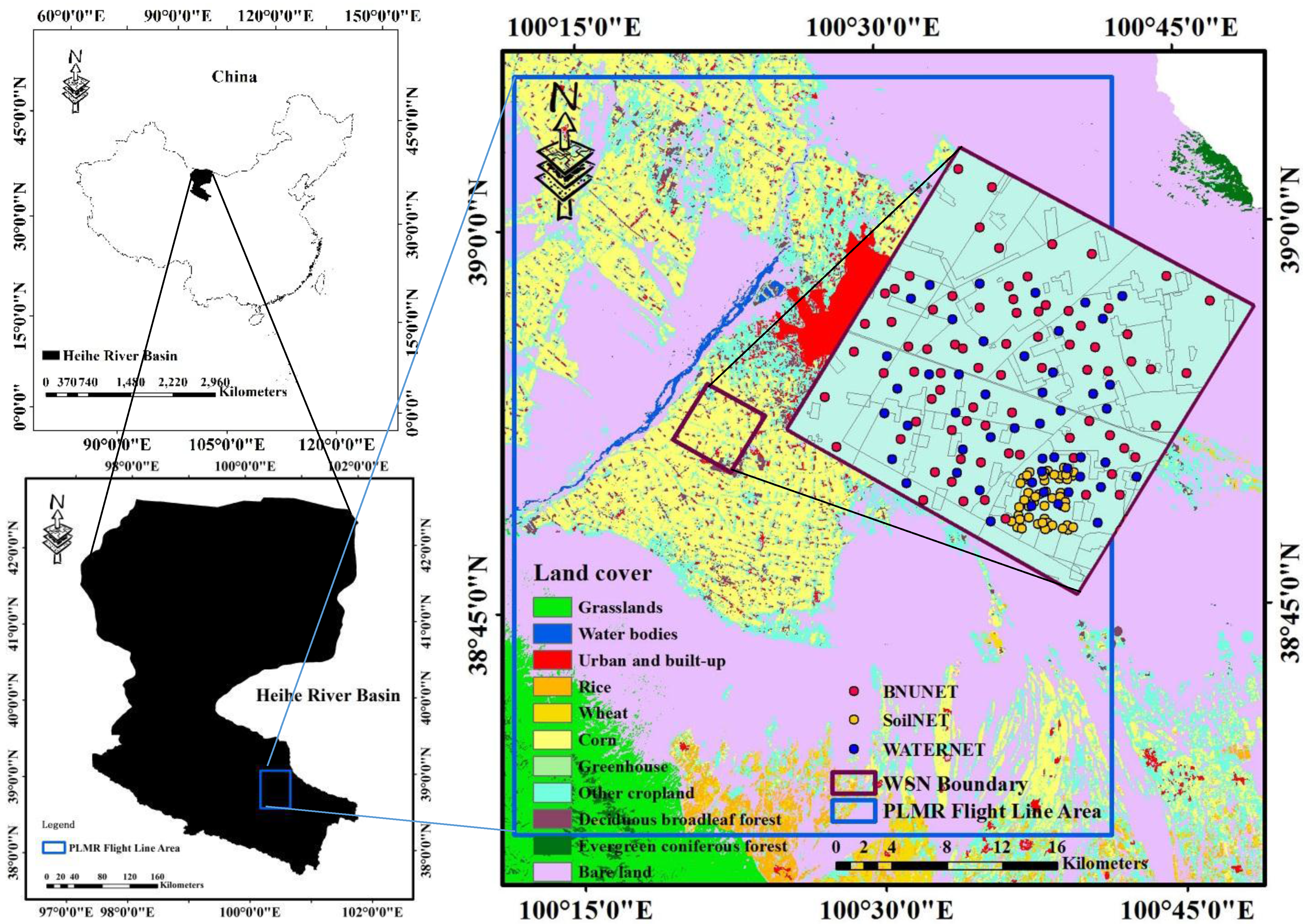
2.1. The Airborne PLMR Microwave Brightness-Temperature Data

The middle sections of the Heihe River Basin represent a key experimental area of the HiWATER experiment. The area is characterized by irrigated oases, and the land cover types include grasslands, urban areas, forests, and bare land [20].

To improve the remote sensing methods for observing key eco-hydrological processes, aircraft-based PLMR and Thermal Airborne Spectrographic Imager (TASI) observations were conducted to measure the BTs across a 50 km × 50 km region in the middle section of the Heihe River Basin (Figure 1). The incidence angles were ±7.5°, ±21.5°, and ±38.5° for the V- and H-polarizations, and measurement details are shown in Table 1. Depending on the observation dates, the flight height ranged from 0.3 to 3 km, and the spatial resolution ranged from 0.1 to 0.75 km. The flight on 2 August did not pass over the study area, and the flight time over the study area on 5 July was short; therefore, the observations from 5 July and 2 August were not used in the study.

Table 1. Measurement details of the PLMR observations.

Observation Date	Flight Height	Spatial Resolution	Data Source
30 June 2012	2.50 km	None	doi:10.3972/hiwater.013.2013.db
3 July 2012	0.35 km	100 m	doi:10.3972/hiwater.014.2013.db
4 July 2012	1.00 km	300 m	doi:10.3972/hiwater.015.2013.db
5 July 2012	2.00 km	600 m	doi:10.3972/hiwater.016.2013.db
7 July 2012	2.00 km	600 m	doi:10.3972/hiwater.017.2013.db
10 July 2012	2.50 km	750 m	doi:10.3972/hiwater.018.2013.db
26 July 2012	2.30 km	700 m	doi:10.3972/hiwater.019.2013.db
1 August 2012	1.00 km	300 m	doi:10.3972/hiwater.020.2013.db
2 August 2012	2.30 km	700 m	doi:10.3972/hiwater.021.2013.db

Table 1. Measurement details of the PLMR observations.

Observation Date	Flight Height	Spatial Resolution	Data Source
30 June 2012	2.50 km	None	doi:10.3972/hiwater.013.2013.db
3 July 2012	0.35 km	100 m	doi:10.3972/hiwater.014.2013.db
4 July 2012	1.00 km	300 m	doi:10.3972/hiwater.015.2013.db
5 July 2012	2.00 km	600 m	doi:10.3972/hiwater.016.2013.db
7 July 2012	2.00 km	600 m	doi:10.3972/hiwater.017.2013.db
10 July 2012	2.50 km	750 m	doi:10.3972/hiwater.018.2013.db
26 July 2012	2.30 km	700 m	doi:10.3972/hiwater.019.2013.db
1 August 2012	1.00 km	300 m	doi:10.3972/hiwater.020.2013.db
2 August 2012	2.30 km	700 m	doi:10.3972/hiwater.021.2013.db

Figure 1. Geographical location of the Heihe River Basin (left), land cover map of the Heihe River Basin [21] and Polarimetric L-band Multibeam Radiometer (PLMR) flight area (right).

Figure 1. Geographical location of the Heihe River Basin (left), land cover map of the Heihe River Basin [21] and Polarimetric L-band Multibeam Radiometer (PLMR) flight area (right).

To facilitate a comparison with satellite products in the future, the PLMR BTs were resampled to raster data with a spatial resolution of 1 km, as shown in Figure 2. This figure shows that for a given angle of incidence, the BTs for V-polarizations were higher than those for H-polarizations. With the incidence angle gradually increasing (from 7.5° to 38.5°), the BTs of H-polarization gradually decreased, whereas those of V-polarization gradually increased. Additionally, the V-polarization BTs at 38.5° were primarily greater than 310 K, which might be caused by radio frequency interference (RFI) [22].

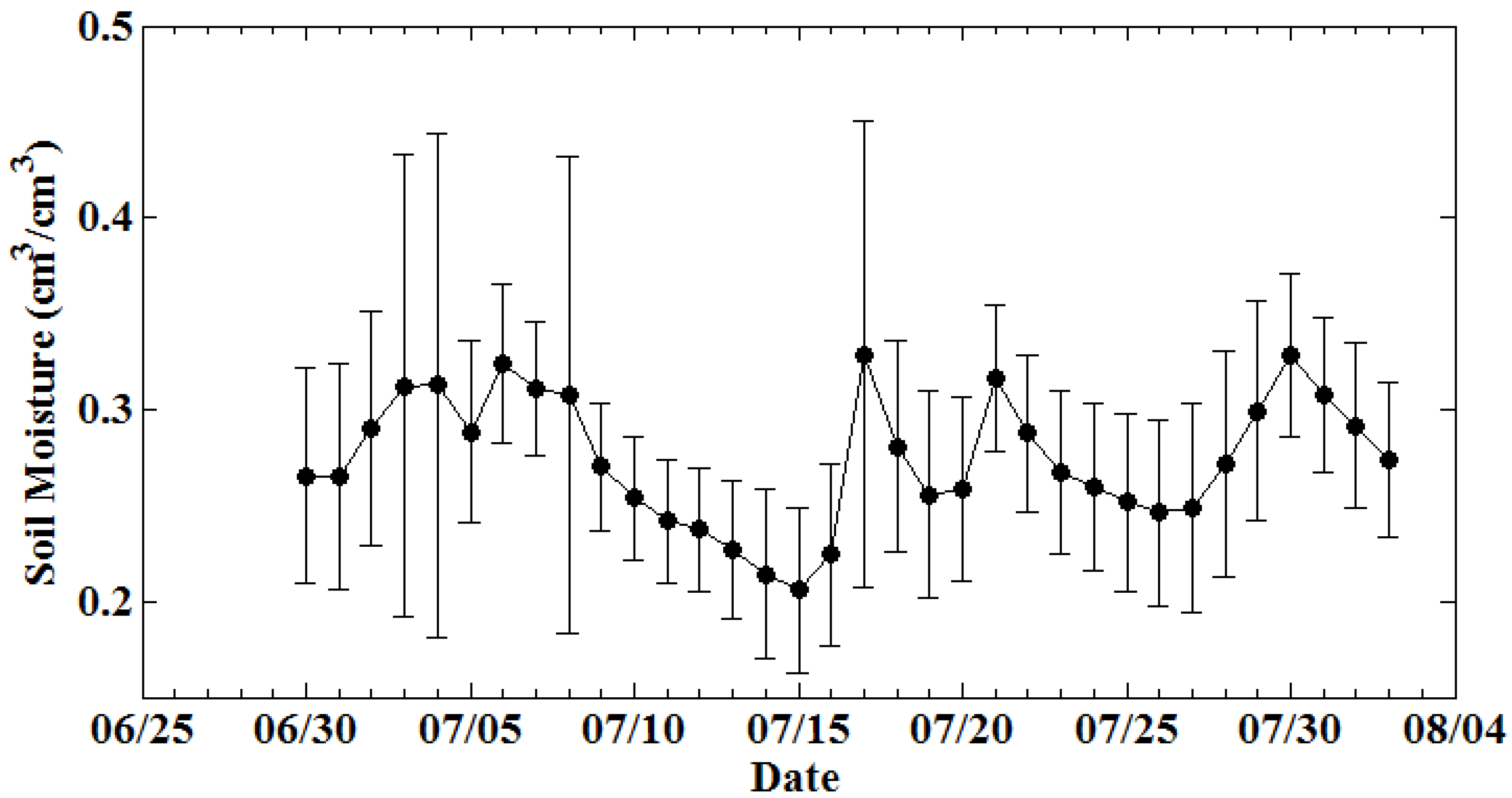
2.2. Field Observation Data

To integrate a variety of hydrological, ecological, and meteorological observation facilities throughout the Heihe River Basin, an eco-hydrological wireless sensor network (WSN) spanning 5.5 km × 5.5 km was established in the middle region [23].

This network includes three types of new sensor nodes: BNUNET [23,24], SoilNET [23,24], and WATERNET [23,24]. The main observation parameters included soil moisture, soil temperature, soil conductivity and the complex dielectric constant. Figure 3 shows the distributions of the three new sensor nodes in the WSN.

The WATERNET datasets were mainly used to simulate BT in this study, and there were 50 WATERNET observation nodes. Except for two nodes implemented in a pea field and orchard, the remaining nodes were all implemented in cornfields. In this study, observations from the two nodes in the pea field and orchard were excluded, and simulations were conducted using data from the cornfield nodes.

Figure 2. PLMR brightness temperature on 30 June 2012, at incidence angle of 7°, 21.5°, and 38.5°for H- and V-polarization during the HiWATER project.

Figure 2. PLMR brightness temperature on 30 June 2012, at incidence angle of 7°, 21.5°, and 38.5°for H- and V-polarization during the HiWATER project.

The observation dates of the WATERNET system ranged from 9 June to 18 September 2012. The observation parameters included soil temperature, soil moisture, soil conductivity and dielectric constants at 4 and 10 cm. When the airborne radiometer passed over the experiment area, the soil surface temperature ranged from 19 °C to 30 °C, whereas the soil moisture ranged from 0.2 to 0.5 cm³/cm³. Additionally, the soil texture data [25] of the Heihe River Basin were used to calculate the dielectric constant of the soil. The LAI data [26] measured in the flux observation matrix were used to calculate the optical depth of the vegetation in the study. The sand and clay contents of the study area were approximately 40% and 10%, respectively.

Figure 3. Geographical location of aircraft observation, land cover map of the aircraft observation area and the distribution of the three types of new sensor nodes in the wireless sensor work (WSN).

Figure 3. Geographical location of aircraft observation, land cover map of the aircraft observation area and the distribution of the three types of new sensor nodes in the wireless sensor work (WSN).

3. The L-MEB Model

As an important forward model in the SMOS soil moisture inversion algorithm, the L-MEB model was composed of four components: bare soil, low vegetation, forest and others. The BT of a pixel was a weighted sum of the four components, expressed as follows [6]:

$${{\displaystyle TB}}_P=f_{bare}·T{B}_{Pbare}+f_{lowveg}·T{B}_{Plowveg}+f_{forest}·T{B}_{Pforest}+f_{other}·T{B}_{Pother}$$

(1)

where TB_P is the BT of an entire pixel, f_* is the proportional area of each component, TB_P* is the BT of each component, and the subscript P represents polarization. The land surface of the study area is primarily covered by crops, and the emissions from a vegetated soil surface are modeled by L-MEB and the τ-ω model as follows [27]:

$${{\displaystyle T}}_B^{model}=\left(1+{{\displaystyle \text{Γ}}}_{soil}^{*}{{\displaystyle r}}_{veg}\right)\left(1-{{\displaystyle r}}_{veg}\right)\left(1-\omega \right){{\displaystyle T}}_{veg}+\left(1-{{\displaystyle \text{Γ}}}_{soil}^{*}\right){{\displaystyle r}}_{veg}{{\displaystyle T}}_{soil}$$

(2)

where T_veg is the vegetation temperature, T_soil is the soil temperature, ${\Gamma }_{soil}^{*}$ is the reflectivity of the soil, ω is the vegetation scattering albedo, and r_veg is the transmissivity of the vegetation layer.

3.1. Soil Effective Temperature

T_soil is an important parameter in Equation (2) that accounts for the contribution of the soil temperature profile to emissions. Based on the radiative transfer theory [28], the effective temperature can be calculated via the following equation:

$${{\displaystyle T}}_{soil}={\displaystyle {\int }_0^{\infty }Ts\left(z\right)}·W\left(z\right)·dz$$

(3)

where Ts(z) is the soil thermodynamic temperature at depth z, and W(z) is a temperature weighting function of the contribution of each soil layer. The latter parameter is defined as follows:

$$W\left(z\right)=\alpha \left(z\right)·\exp \left[-{\displaystyle {\int }_0^z\alpha \left(z^{\prime }\right)}·dz\prime \right]$$

(4)

$$\alpha \left(z\right)=\left(\frac{4\pi }{\lambda }\right)·\frac{Ei\left(z\right)}{2{\left(Er\left(z\right)\right)}^{0.5}}$$

(5)

where α(z) is an attenuation coefficient related to the soil dielectric constant, λ is the observed wavelength, and Er and Ei are the real and imaginary soil dielectric constant variables, respectively. This method details the influence of several temperatures at different soil layers on the soil’s total radiation, but the calculation is not easily implemented. For applied studies at a large scale, simple parameterizations are necessary. The most straightforward parameterization was proposed by Choudhury et al. [29]:

$${{\displaystyle T}}_{soil}={{\displaystyle T}}_{deep}+\left({{\displaystyle T}}_{surf}-{{\displaystyle T}}_{deep}\right)·Ct$$

(6)

where T_deep is the deep soil temperature (10 cm in this study), T_surf is the surface temperature (approximately over a depth of 0–5 cm), and Ct is an adjustable parameter that is affected by the observation frequency and soil moisture. This adjustable parameter can be calculated using the imaginary (Ei) and real (Er) soil dielectric constant variables [30]:

$$Ct={\left(\frac{Ei/Er}{E0}\right)}^{b0}$$

(7)

where E0 and b0 are empirical parameters that depend on specific soil characteristics. In the study, T_surf and T_deep are equal to the soil temperature at 4 and 10 cm, respectively, as measured by the WATERNET system; E0 = 0.3 and b0 = 0.3 are set as the default values.

3.2. Soil Reflectivity

Soil reflectivity is calculated using the Q-H model proposed by Wang and Choudhury [31]:

$${{\displaystyle \text{Γ}}}_{soil}^{*}=\left[\left(1-Qs\right){{\displaystyle R}}_P^{*}\left(\text{θ}\right)+Qs{{\displaystyle R}}_Q^{*}\left(\text{θ}\right)\right]·\exp \left(-h·{\cos }^{{{\displaystyle N}}_P}\left(\text{θ}\right)\right)$$

(8)

where $R_P^{*}\left(\theta \right)$ and $R_Q^{*}\left(\theta \right)$ are Fresnel reflectance values. Qs and h are the semi-empirical parameters that model the intensity of the roughness effects and the polarization-mixing effects, respectively. The parameter N_P is an exponent that is affected by polarization mode, θ is the observation angle, and P is polarization. Qs, N_H and N_V are set to zero, as indicated by published studies based on large experimental datasets [32].

In earlier research, the h parameter was found to be correlated with the slope parameter (the standard deviation in surface height (S_D) and the associated correlation length (L_C)) and the surface soil moisture [33]. Based on a new method proposed by Escorihuela et al., the h parameter depends on the soil moisture as follows [34]:

$$h=\{\begin{array}{l}2{\left(k\sigma \right)}^2-4.4·\left(ws-w{s}_{FC}\right),ws\le w{s}_{FC}\\ 2{\left(k\sigma \right)}^2,ws>w{s}_{FC}\end{array}$$

(9)

where k is the wavenumber, and σ is the root-mean-square (RMS) height. The RMS height was not measured during the HiWATER experiments. Therefore, the RMS height is a fitting parameter that compares TB simulations and PLMR observations. In addition, because the simulation was conducted at the corn surface with row structure, the RMS height value could be larger [35]. Hence, an RMS height of 1.5 cm was derived as a fitting parameter. ws is soil moisture, and WS_FC is the field capacity related to soil texture.

3.3. Vegetation Effects

Vegetation layer transmissivity r_veg is calculated from the vegetation optical depth τ by accounting for the variation in the vegetation slant height angle:

$${{\displaystyle r}}_{veg}=\exp \left(-\text{τ}\sec \text{θ}\right)$$

(10)

The vegetation optical thickness τ, calibrated by Wigneron et al., depends on observation θ and polarization P, written as follows [36]:

$$\text{τ}\left(\text{θ},h\right)=\mathrm{constant}$$

(11)

$$\text{τ}\left(\text{θ},v\right)=\text{τ}\left(\text{θ},\text{h}\right)\left({\cos }^2\text{θ}+Cpol {\sin }^2\text{θ}\right)$$

(12)

where Cpol is a correction parameter. Jackson et al. [37] indicated that vegetation (such as corn, soybeans, and alfalfa) optical thickness is generally linearly related to the total vegetation water content (VWC), and ignored the effect of polarization on optical thickness. Cpol can then be set to 1 as the default value, i.e., ignoring the polarization effect of optical thickness.

Vegetation optical thickness for H-polarization is generally linearly related to VWC (kg/m²) using the b parameter [38]:

$$\text{τ}=b·VWC$$

(13)

VWC is correlated with the LAI for crop-covered surfaces and can be expressed as follows [6]:

$$VWC=0.5·LAI$$

(14)

The values of b and ω have been calibrated for different crop types by Wigneron et al. [13]. The study area is covered with corn, thus, b = 0.15 and ω = 0.06 are set as the model’s default parameters in this study.

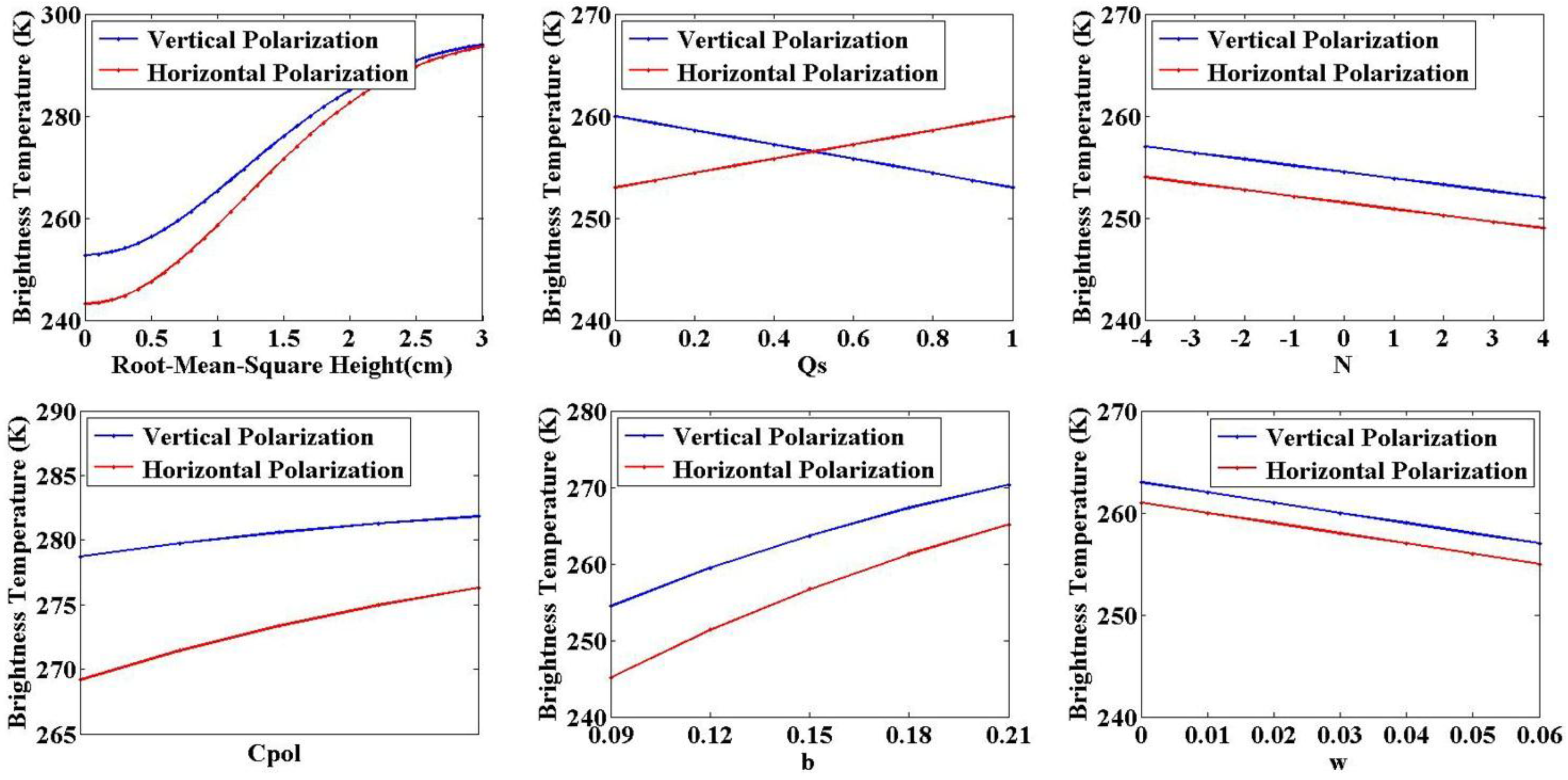
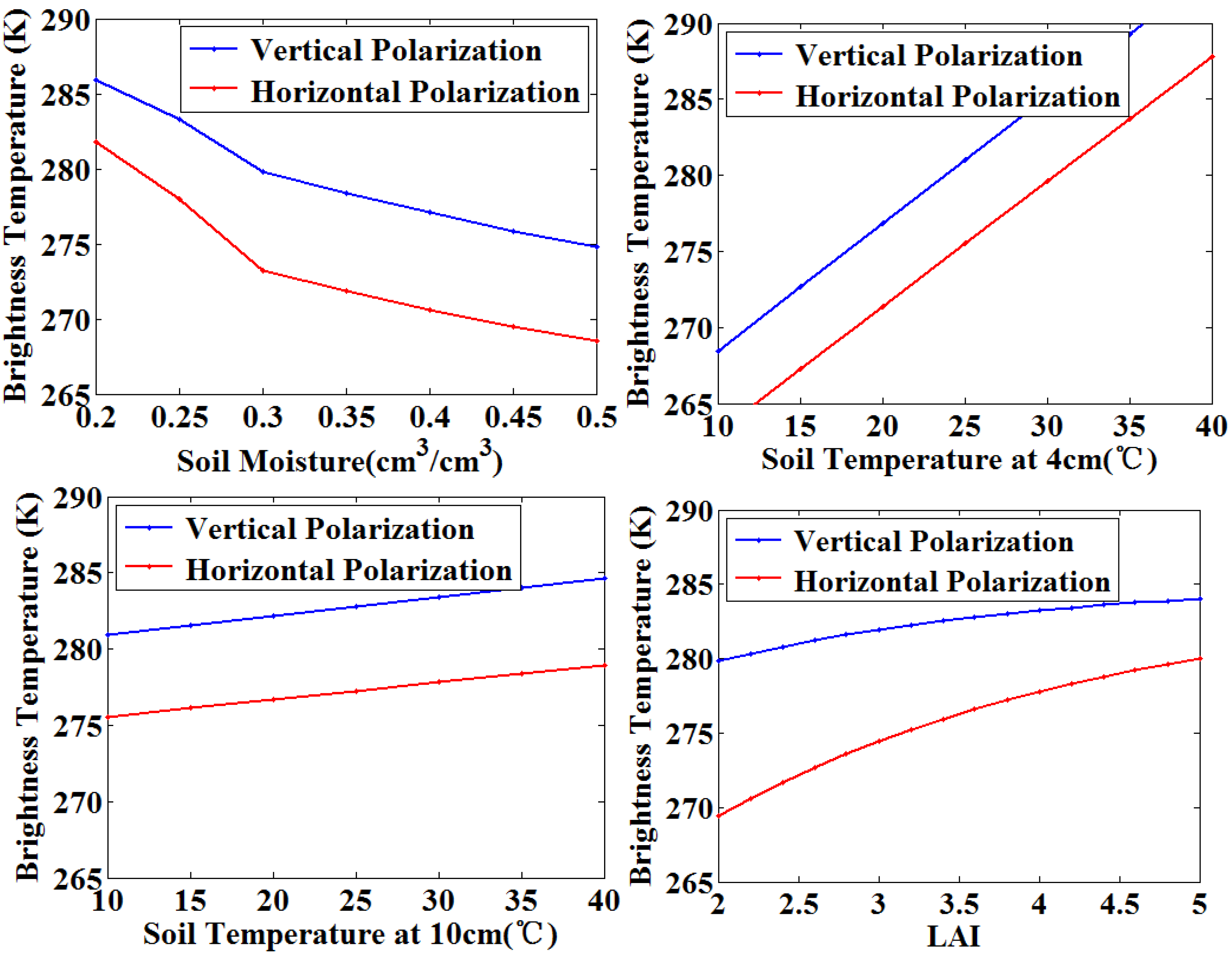
4. Sensitivity Analysis of L-MEB

According to the above description of the L-MEB model, many studies have calibrated the parameters of the L-MEB model for different areas. However, these calibrated parameters of the L-MEB model may not be suitable for the Heihe River Basin, and were thus recalibrated. For a reasonable calibration, the features of the L-MEB model must be determined. A sensitivity analysis of the model was thus conducted. In this study, the BTs of the vegetation canopy were simulated, and the microwave radiation signal received by the airborne sensors was detected. This signal derived mainly from soil and vegetation, which are influenced by underlying surface roughness, soil moisture, soil texture, vegetation temperature, VWC, and LAI. The input parameters of the model can be divided into two categories: (a) ground observation parameters, such as soil moisture, soil temperature and LAI; and (b) semi-empirical parameters, such as Qs, N_H, N_V, Cpol, b and ω.

Table 2. Ranges of the ground observation parameters in WATERNET.

Input Parameter	Ranges	Mean
soil moisture (cm3/cm3)	0.14–0.46	0.26
Soil temperature at 4 cm (°C)	21.86–38.04	27.42
Soil temperature at 10 cm (°C)	18.85–29.44	23.94
LAI	1.75–5.25	3.50

Table 2. Ranges of the ground observation parameters in WATERNET.

Input Parameter	Ranges	Mean
soil moisture (cm3/cm3)	0.14–0.46	0.26
Soil temperature at 4 cm (°C)	21.86–38.04	27.42
Soil temperature at 10 cm (°C)	18.85–29.44	23.94
LAI	1.75–5.25	3.50

Based on the observed data from the study area; the soil moisture; soil temperature and LAI ranges used in the model were set according to Table 2. Because there were no obvious differences between surface temperature and vegetation temperature in the study area, vegetation temperature is assumed to be equal to surface temperature. The soil texture in the model was set to a constant value (sand = 0.35; clay = 0.08); and other semi-empirical parameters were set to default values.

Figure 4 shows that with an increase in soil moisture, the BTs significantly decrease for both polarizations. Furthermore, with an increase in soil temperature at 4 cm, the BTs significantly increase for both polarizations. The model is much less sensitive to the soil temperature at 10 cm. The principal components of the sensor’s surface microwave radiation reception are attributable to the soil effective temperature and vegetation temperature, and the soil effective temperature is mainly affected by soil moisture and soil surface temperature. Therefore, soil temperature at 4 cm and soil moisture are crucial to the simulations.

The semi-empirical parameters that required adjustment included Qs, N_H, N_V, Cpol, b and ω. Based on multiple experiments, Qs and N_P range from 0 to 1 and –4 to 4, respectively, and Qs tends to be 0 at low frequencies [32,39,40]. At 1.4 GHz, b = 0.12 ± 0.03 is suitable for most crop types [6], and omega is approximately 0.06 for corn [13]. Cpol represents the correction parameter, which is equal to 1 and 2.6 for soybeans and wheat, respectively [36]. Cpol in this study ranged from 1 to 3. The RMS height was set as a fitting parameter in the study, and the influence of the RMS height on the simulated BT was also analyzed, as shown in Figure 5.

Figure 4. The effects of ground observation data including soil moisture, soil temperature (4 cm and 10cm), and LAI on the modeled BT at L-band.

Figure 4. The effects of ground observation data including soil moisture, soil temperature (4 cm and 10cm), and LAI on the modeled BT at L-band.

Figure 5. The effects of fitting parameter and semi-empirical parameters on the modeled BT at L-band.

Figure 5. The effects of fitting parameter and semi-empirical parameters on the modeled BT at L-band.

The sensitivity analysis of the model with respect to the semi-empirical parameters showed that the L-MEB model was more sensitive to the RMS height and N (N_H and N_V). With an increase in RMS height, the BTs of both polarizations gradually increased. When the soil roughness increased, soil reflectance decreased, and soil emissivity increased; therefore, the radiation of the surface increased. With an increase in Qs, the V-polarization BTs decreased and the H-polarization BTs increased, as shown in Figure 5.

5. Results and Discussion

5.1. Calibration of the Semi-Empirical Parameters

According to the model’s sensitivity, the above semi-empirical parameters could be appropriately adjusted with ranges referenced in previous studies [6,13,32,36,39,40]. Calibration was based on minimizing the difference between the L-MEB modeled BTs and the PLMR measurements.

Because each observation node stored WATERNET data, the simulation results were aggregated to a 1 km spatial resolution to match the airborne PLMR data. However, during the simulation process, two resampling methods could be used to obtain a simulated BT: (1) simulation from point observations (soil moisture, soil temperature, LAI, etc.). In this case, the simulated BT of each point observation was initially calculated, and the simulated BT was then resampled at a 1 km resolution; (2) Simulation based on gridded field data with a resolution of 1 km averaged from the point observations. In this method, the ground parameters (soil moisture, soil temperature, LAI, etc.) were initially resampled at a 1 km resolution. The simulation was then conducted using the L-MEB model based on these gridded field data, and the simulated BTs at a 1 km resolution were obtained. It should be noted that because there may be several point observations within one pixel, the arithmetic average method, which is the simplest, most convenient and most frequently used method of all calculations for area-averaged parameters, was used to calculate the gridded data at a 1 km resolution [40,41,42,43,44,45].

The differences between the two resampling methods were mainly related to the different resample objects and times. In this study, one method was applied to the BT after the simulation process (Method 1), whereas the other method was applied to the ground parameters before the simulation process (Method 2). It can be assumed that the simulation process was also an error propagation process. Because soil moisture was the most sensitive parameter to BT, it can be expected that the overall relationship between BT and the parameters was mainly affected by soil moisture. In this study, the average soil moisture of the ground observations ranged from 0.21 to 0.33 cm³/cm³, as shown in Figure 6, and the relationship between simulated BT and soil moisture tended to be an upward parabola in this range, as shown in Figure 4. Therefore, we assumed that the overall relationship between BT and all parameters could be represented using a concave upward parabola, as shown in Figure 7.

To analyze the differences between the two resampling methods, a mathematical strategy was used in which we assumed that there were only two point observations in one pixel and the observation error for each point was ψ₁ and ψ₂. After the simulation process, which can also be observed as an error propagation process, ψ₁ and ψ₂ were amplified into y₁ and y₂, as shown in Figure 7. Using Method 2, the area-averaged observation error was₀ and transferred into f(ψ₀) after the simulation process, whereas using Method 1, the final error corresponded to the average simulated BT error y₀. It was obvious that f(ψ₀) was smaller than y₀, which indicated that Method 2 was more accurate than Method 1.

Figure 6. Temporal evolution of mean soil moisture content calculated from the average of ground observations. Vertical bars correspond to the standard deviation of the soil moisture.

Figure 6. Temporal evolution of mean soil moisture content calculated from the average of ground observations. Vertical bars correspond to the standard deviation of the soil moisture.

Figure 7. The mathematical expression of two resampling methods.

Figure 7. The mathematical expression of two resampling methods.

Through the above analysis, it can be concluded that the resampling strategy was related to the uniformity of the observations. If the observations were uniform, e.g., ψ₁ =ψ₂, then f(ψ₀) = y₀. However, based on the analysis of the WATERNET observations shown in Figure 6, the standard deviation varied between 0.03 and 0.13 cm³/cm³. Thus, soil moisture variability within the study area was high. Therefore, the resampling method based on gridded data was used in this study.

Based on ground observation data, the simulation results were calculated using the L-MEB model with a resampling method based on gridded data. The results were compared to the PLMR data on 30 June, 3 July, 4 July, 26 July and 2 August 2012 to calibrate the semi-empirical parameters. The calibrated model parameters that were suitable for the study area are shown in Table 3. Calibrated Qs, N_H, N_V, Cpol, b and ω values were similar to previous results. Cpol was greater than 1, and Equations (11) and (12) indicated that the vegetation optical thickness at V-polarization was larger than that at H-polarization and that vegetation transmissivity would be lower and canopy emissivity (1−ω)(1−γ) would be higher at V-polarization. This result can be attributed to the vertical structure of corn. At L-band, the influence of vertically oriented canopy elements, i.e., corn stalks, plays a greater role in scattering and absorption.

Table 3. Calibrated parameters using the resampling method based on the gridded data.

Qs	NH	NV	Cpol	b	ω
0.0	–1.0	–4.0	3.0	0.12	0.05

Table 3. Calibrated parameters using the resampling method based on the gridded data.

Qs	NH	NV	Cpol	b	ω
0.0	–1.0	–4.0	3.0	0.12	0.05

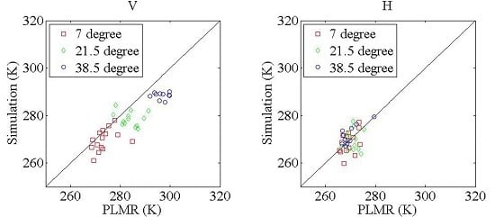
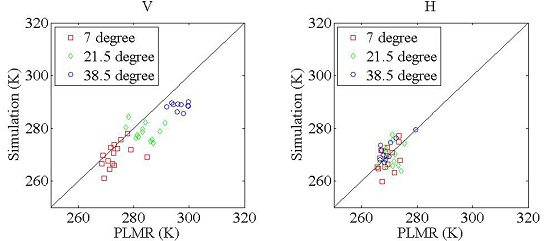
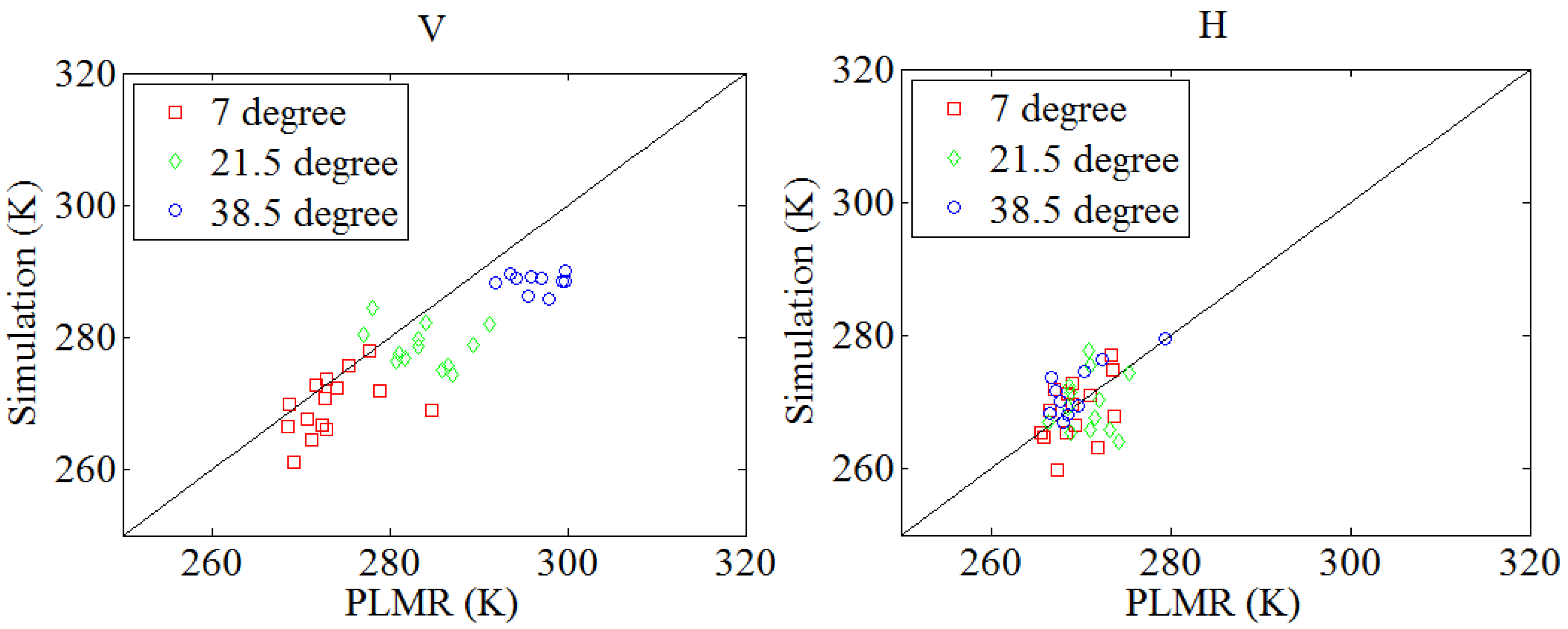
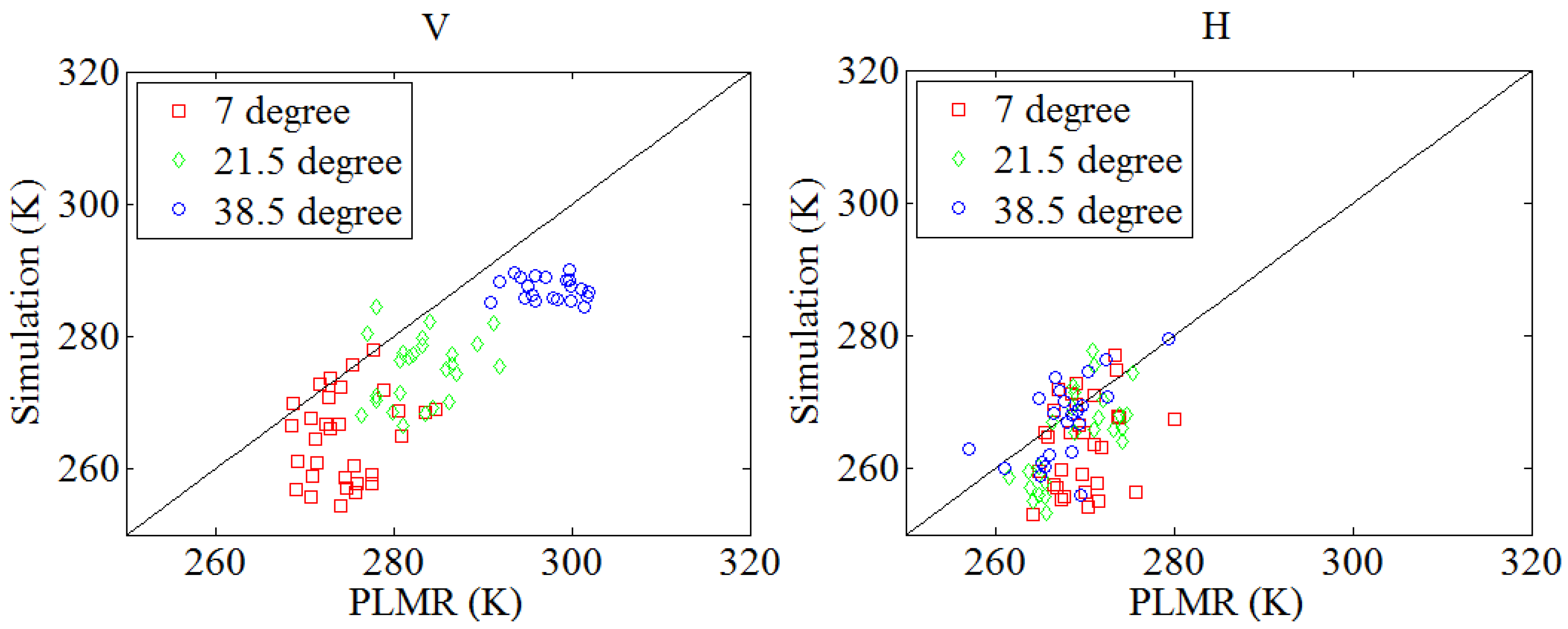
5.2. Validation of the Calibrated Parameters

In this study, the PLMR data on 7 and 10 July 2012 were used to validate the calibrated parameters. Figure 8 shows scatterplots of the simulation results against the PLMR data at different incidence angles for both polarizations on 7 and 10 July 2012. Both the BT of the PLMR data and the simulation results at V-polarization tended to increase with an increase in incident angle (7°–38.5°), whereas there were no obvious differences for H-polarization at different angles. This result could be attributed to the land cover of the study area. According to previous studies [46], for bare land, the emissivity at V-polarization would increase with an increase in the incident angle from 7° to 38.5°, whereas emissivity would decrease at H-polarization. However, when the surface is covered with corn, the vertical stalks dominate the scattering pattern within the corn canopy and increase surface emissivity at both polarizations. Therefore, emissivity of the corn’s surface increases with increases in incidence angle at V-polarization but not H-polarization. Table 4 shows the RMSE and R (the correlation coefficient) values. The results were 12.15 K (9.24 K) at an incidence angle of 7°, 9.05 K (5.83 K) at 21.5°, and 9.16 K (4.06 K) at 38.5° at V-polarization (H-polarization). R was approximately 0.180 (0.264) at an incidence angle of 7°, 0.241 (0.696) at 21.5°, and –0.116 (0.614) at 38.5° at V-polarization (H-polarization). The simulation results at H-polarization were more accurate, whereas the correlation between PLMR data and the simulation results was not adequate at V-polarization. This result was mainly attributed to the influence of RFI on the PLMR observations at V-polarization, according to the metadata.

Figure 8. Comparison of the PLMR data and simulation results at three incidence angles for both polarizations on 7 and 10 July 2012.

Figure 8. Comparison of the PLMR data and simulation results at three incidence angles for both polarizations on 7 and 10 July 2012.

Table 4. RMSE and R between the PLMR data and the simulation results on 7 and 10 July 2012.

θ	RMSE (V)	RMSE (H)	R (V)	R (H)
7°	12.15 K	9.24 K	0.180	0.264
21.5°	9.05 K	5.83 K	0.241	0.696
38.5°	9.16 K	4.06 K	–0.116	0.614

Table 4. RMSE and R between the PLMR data and the simulation results on 7 and 10 July 2012.

θ	RMSE (V)	RMSE (H)	R (V)	R (H)
7°	12.15 K	9.24 K	0.180	0.264
21.5°	9.05 K	5.83 K	0.241	0.696
38.5°	9.16 K	4.06 K	–0.116	0.614

The LAI data used in this study were from ground measurements, and for the lack of data on 7 July, the LAI data used to simulate the BT on 7 July were identical to those for 5 July, which indicates that the LAI data for 7 July might be underestimated and might influence validation accuracy. According to the effect of LAI on the simulations, as shown in Figure 4, the simulated BT tended to increase with an increase in LAI, which indicates that an underestimation of LAI would lead to an underestimation of the simulation results. Therefore, the 7 July simulations were removed in the final validation. Figure 9 shows the scatterplots of the simulation results against the PLMR data at different incidence angles for both polarizations on 10 July. Table 5 shows the RMSE and R (the correlation coefficient) values of the results. The results were 6.05 K (4.23 K) at an incidence angle of 7°, 7.26 K (4.67 K) at 21.5°, and 7.05 K (2.70 K) at 38.5° at V-polarization (H-polarization).

As can be seen in Table 5, the RMSEs are lower and at a relatively reasonable accuracy. In addition, in Figure 9, it can be seen that when putting together all of data at three incidence angles, the simulations show a good correlation with the observations both at H and V polarization. However, if we analyze the correlation at the view of each angle, the amount of data is limited. R was approximately 0.438 (0.460) at an incidence angle of 7°, –0.208 (0.038) at 21.5°, and –0.008 (0.779) at 38.5° at V-polarization (H-polarization). The values at each angle almost concentrated in a small range, which finally influence the R value, and leading to that R was lower than 0.50 in most cases. Nevertheless, relatively speaking, due to the RFI influence, the R of V-polarization at 21.5° and 38.5° also show lower values than most of the other cases.

Table 5. RMSE and R between the PLMR data and the simulation results on 10 July 2012.

θ	RMSE (V)	RMSE (H)	R (V)	R (H)
7°	6.05 K	4.23 K	0.438	0.460
21.5°	7.26 K	4.67 K	−0.208	0.038
38.5°	7.05 K	2.70 K	−0.008	0.779

Table 5. RMSE and R between the PLMR data and the simulation results on 10 July 2012.

θ	RMSE (V)	RMSE (H)	R (V)	R (H)
7°	6.05 K	4.23 K	0.438	0.460
21.5°	7.26 K	4.67 K	−0.208	0.038
38.5°	7.05 K	2.70 K	−0.008	0.779

It should be noted that some PLMR values were higher than 305 K at V-polarization at an incidence of 38.5°. Based on the WATERNET measurements, the soil temperature at 4 cm ranged from 21.86 °C to 38.04 °C, and the average value was approximately 30 °C (303 K). The surface emissivity was assumed to be 1; thus, the highest BT was 303 K. Consequently, the PLMR values that were larger than 303 K are problematic. Therefore, in the final simulation, BTs greater than 303 K were removed.

Figure 9. Comparison of the PLMR data and simulation results at three incidence angles for both polarizations on 10 July 2012.

Figure 9. Comparison of the PLMR data and simulation results at three incidence angles for both polarizations on 10 July 2012.

6. Conclusions

In this study, a calibration of the semi-empirical parameters in L-MEB model has been implemented over the middle region of the Heihe River Basin in Northern China. In the process, the ground observations, including soil moisture, temperature and texture, from the HiWATER project were used as input parameters of L-MEB model. The model calibration was conducted by minimizing the difference between the L-MEB simulated BTs and the airborne PLMR measurements on 30 June, 3 July, 4 July, 26 July and 2 August 2012. The semi-empirical parameters of L-MEB model were acquired and validated by the PLMR data on 10 July. In the validation process, the RMSE between the simulations and measurements were 6 to 7 K for V-polarization and 2.7 to 4.7 K for H-polarization at different angles. This work demonstrated that the calibrated parameters of the L-MEB model are suitable for this region.

In order to match the grid resolution of airborne PLMR data, point data were processed with the area-averaged method to represent the grid value. There were two methods to aggregate point measurements into airborne brightness temperature simulation. One simulation at the airborne scale was conducted from the area-averaged surface parameters (soil moisture, soil temperature and soil texture). The other was derived from the averaging point simulated BTs at field scale. It was found that simulations based on the area-averaged surface parameters showed a relative smaller error. It is because that simulated BT was a nonlinear decreasing function of surface soil moisture. The grid TB simulation based on spatial average of ground parameters was closer to PLMR value, compared with aggregated TB simulation at point measurements.

Meanwhile, it should be noted was that some errors still exist in the validation. Three possible explanations for these results are as follows: (a) During the PLMR observations, pitch and rotation frequently occurred, and RFI also occurred at the largest incidence angle (38.5°) at the V-polarization [8], thus leading to uncertainty in the observations; (b) It is notable that RMS height was set a constant during the model simulation. However, the value might change across pixels for an expansive study area. This assumption might affect the final simulations accuracy; (c) The standard deviation of soil moisture in the study area was more than 0.1, the maximum could be up to 0.3. This indicated a relative large spatial heterogeneity of the surface soil moisture. Although the area-averaged method was used to reduce the influence of the spatial heterogeneity on the simulations, the area-averaged soil moisture used in the simulation would cause errors in the simulation. It is still a challenge to estimate the upscaled pixel-averaged soil moisture based on point observations on the ground, especially for those areas with large spatial heterogeneity.

Overall, the calibration of L-MEB in this study performed reasonable simulation over the crop-covered land surface. The calibrated parameters could be used in future applications of L-MEB for soil moisture retrieval over arid areas with similar terrains and climatology. Further study is needed to focus on estimations of pixel-averaged soil moisture using in situ moisture measurements.

References

1. Delworth, T.; Manabe, S. The influence of potential evaporation on the variability of simulated soil wetness and climate. J. Clim. 1988, 13, 2900–2922. [Google Scholar] [CrossRef]
2. Kachi, M.; Fujii, H.; Murakami, H.; Hori, M.; Ono, A.; Igarashi, T.; Nakagawa, K.; Oki, T.; Honda, Y.; Shimoda, H. Global change observation mission (GCOM) for monitoring carbon, water cycles, and climate change. Proc. IEEE 2010, 98, 717–734. [Google Scholar]
3. Kerr, Y.H.; Waldteufel, P.; Wigneron, J.P.; Martinuzzi, J.M.; Font, J.; Berger, M. Soil moisture retrieval from space: The Soil Moisture and Ocean Salinity (SMOS) mission. IEEE Trans. Geosci. Remote Sens. 2001, 39, 1729–1735. [Google Scholar] [CrossRef]
4. Njoku, E.G.; O'Neill, P.E.; Kellogg, K.H.; Crow, W.T.; Edelstein, W.N.; Entin, J.K.; Goodman, S.D.; Jackson, T.J.; Johnson, J.; Kimball, J.; et al. The soil moisture active passive (SMAP) mission. Proc. IEEE 2010, 98, 704–716. [Google Scholar]
5. Koblinsky, C.J.; Hildebrand, P.; LeVine, D.; Pellerano, F.; Chao, Y.; Wilson, W.; Yueh, S.; Lagerloef, G. Sea surface salinity from space: Science goals and measurement approach. Radio Sci. 2003, 38. [Google Scholar] [CrossRef]
6. Wigneron, J.P.; Pellarin, T.; Calvet, J.C.; de Rosnay, P.; Kerr, Y.H. Surface emission. In Thermal Microwave Radiation: Applications for Remote Sensing; The Institution of Engineering and Technology: London, UK, 2006; pp. 362–371. [Google Scholar]
7. Pellarin, T.; Wigneron, J.P.; Calvet, J.C.; Berger, M.; Douville, H.; Ferrazzoli, P.; Kerr, Y.H.; Lopez-Baeza, E.; Pulliainen, J.; Simmonds, L.P.; et al. Two-year global simulation of L-band brightness temperatures over land. IEEE Trans. Geosci. Remote Sens. 2003, 41, 2135–2139. [Google Scholar] [CrossRef]
8. Li, D.Z.; Jin, R.; Zhou, J. Analysis and reduction of the uncertainties in soil moisture estimation with the L-MEB model using EFAST and ensemble retrieval. IEEE Geosci. Remote Sens. Lett. 2015, 12, 1337–1341. [Google Scholar] [CrossRef]
9. Wigneron, J.P.; Kerr, Y.H.; Waldteufel, P.; Saleh, K.; Escorihuela, M.J.; Richaume, P.; Ferrazzoli, P.; de Rosnay, P.; Gurney, R.; Calvet, J.C.; et al. L-band microwave emission of the biosphere (L-MEB) model description and calibration against experimental data sets over crop fields. Remote Sens. Environ. 2007, 107, 639–655. [Google Scholar] [CrossRef]
10. Grant, J.P.; Saleh, K.; Wigneron, J.P.; Guglielmetti, M.; Kerr, Y.H.; Schwank, M.; Skou, N.; de Griend, A. Calibration of the L-MEB model over a coniferous and a deciduous forest. IEEE Trans. Geosci. Remote Sens. 2008, 46, 808–818. [Google Scholar] [CrossRef]
11. Saleh, K.; Wigneron, J.P.; de Rosnay, P.; Calvet, J.C.; Kerr, Y.H. Semi-empirical regressions at L-band applied to surface soil moisture retrievals over grass. Remote Sens. Environ. 2006, 101, 415–426. [Google Scholar] [CrossRef]
12. Ferrazzoli, P.; Guerriero, L.; Wigneron, J.P. Simulating L-band emission of forests in view of future satellite applications. IEEE Trans. Geosci. Remote Sens. 2002, 40, 2700–2708. [Google Scholar] [CrossRef]
13. Wigneron, J.P.; Pardé, M.; Waldteufel, P.; Chanzy, A.; Kerr, Y.H.; Schmidl, S.; Skou, N. Characterizing the dependence of vegetation model parameters on crop structure, incidence angle, and polarization at L-band. IEEE Trans. Geosci. Remote Sens. 2004, 42, 416–425. [Google Scholar] [CrossRef]
14. Mialon, A.; Coret, L.; Kerr, Y.H.; Sécherre, F.; Wigneron, J.P. Flagging the topographic impact on the SMOS signal. IEEE Trans. Geosci. Remote Sens. 2008, 46, 689–694. [Google Scholar] [CrossRef] [Green Version]
15. Mugnai, A.; Cooper, H.J.; Smith, E.A.; Tripoli, G.J. Simulation of microwave brightness temperature of an evolving hailstorm at SSM/I frequencies. Bull. Am. Meteorol. Soc. 1990, 71, 2–13. [Google Scholar] [CrossRef]
16. Adler, R.F.; Yeh, H.M.; Prasad, N.; Tao, W.K.; Simpson, J. Microwave simulations of a tropical rainfall system with a three-dimensional cloud model. J. Appl. Meteorol. 1991, 30, 924–953. [Google Scholar] [CrossRef]
17. Lin, B.; Wielicki, B.; Minnis, P.; Rossow, W. Estimation of water cloud properties from satellite microwave, infrared and visible measurements in oceanic environments: 1. Microwave brightness temperature simulations. J. Geophys. Res. 1998, 103, 3873–3886. [Google Scholar] [CrossRef]
18. Li, X.; Cheng, G.D.; Liu, S.M.; Xiao, Q.; Ma, M.G.; Jin, R.; Che, T.; Liu, Q.H.; Wang, W.Z.; Qi, Y.; et al. Heihe Watershed Allied Telemetry Experimental Research (HiWATER): Scientific objectives and experimental design. Bull. Am. Meteorol. Soc. 2013, 94, 1145–1160. [Google Scholar] [CrossRef]
19. Cheng, G.D.; Li, X.; Zhao, W.Z.; Xu, Z.H.; Feng, Q.; Xiao, S.C.; Xiao, H.L. Integrated study of the water-ecosystem-economy in the Heihe River Basin. Natl. Sci. Re. 2014, 1, 413–428. [Google Scholar] [CrossRef]
20. Zhang, J.H.; Li, G.D.; Nan, Z.R.; Xiao, H.L.; Zhao, Z.S. The spatial distribution of soil organic carbon storage and change under different land uses in the middle of Heihe River. Sci. Geogr. Sin. 2011, 31, 982–988. [Google Scholar]
21. Zhong, B.; Ma, P.; Nie, A.H.; Yang, A.X.; Yao, Y.J.; Lv, W.B.; Zhang, H.; Liu, Q.H. Land cover mapping using time series HJ-1/CCD Data. Sci. China Earth Sci. 2014, 57, 1790–1799. [Google Scholar] [CrossRef]
22. Li, D.Z.; Jin, R.; Che, T.; Walker, J.; Gao, Y.; Ye, N.; Wang, S.G. Soil moisture retrieval from airborne PLMR products in the Zhangye oasis of middle stream of Heihe River basin, China. Adv. Earth Sci. 2014, 29, 295–305. [Google Scholar]
23. Jin, R.; Li, X.; Yan, B.P.; Li, X.H.; Luo, W.M.; Ma, M.G.; Guo, J.W.; Kang, J.; Zhu, Z.L. A nested eco-hydrological wireless sensor network for capturing surface heterogeneity in the middle-reach of Heihe River basin, China. IEEE Geosci. Remote Sens. Lett. 2014, 11, 2015–2019. [Google Scholar] [CrossRef]
24. Kang, J.; Li, X.; Jin, R.; Ge, Y.; Wang, J.; Wang, J. Hybrid optimal design of the eco-hydrological wireless sensor network in the middle reach of the Heihe River Basin, China. Sensors 2014, 14, 19095–19114. [Google Scholar] [CrossRef] [PubMed]
25. Ma, M.G.; Chen, Y.Y.; Wang, X.F.; Han, H.B.; Yu, W.P.; Wang, H.B.; Shang, H.L. HiWATER: Dataset of Soil Parameters in the Middle Reaches of the Heihe River Basin; Heihe Plan Science Data Center: Lanzhou, China, 2013. [Google Scholar] [CrossRef]
26. Qu, Y.H.; Zhu, Y.Q.; Han, W.C. HiWATER: Dataset of LAINet Observations in the Middle Reaches of the Heihe River Basin; Institute of Remote Sensing Applications, Beijing Normal University: Beijing, China, 2012. [Google Scholar] [CrossRef]
27. Panciera, R.; Walker, J.P.; Kalma, J.; Kim, E. A proposed extension to the soil moisture and ocean salinity level 2 algorithm for mixed forest and moderate vegetation pixels. Remote Sens. Environ. 2011, 115, 3343–3354. [Google Scholar] [CrossRef]
28. Ulaby, F.; Moore, R.; Fung, A.K. Microwave Remote Sensing Active and Passive-Volume III: From Theory to Applications; Artech House: Norwood, UK, 1986. [Google Scholar]
29. Choudhury, B.; Schmugge, T.; Mo, T. A parameterization of effective soil temperature for microwave emission. J. Geophys. Res. 1982, 87, 1301–1304. [Google Scholar] [CrossRef]
30. Holmes, T.R.H.; de Rosnay, P.; de Jeu, R.; Wigneron, J.P.; Kerr, Y.H.; Calvet, J.C.; Escorihuela, M.J.; Saleh, K.; Lemaître, F. A new parameterization of the effective temperature for L band radiometry. Geophys. Res. Lett. 2006, 33. [Google Scholar] [CrossRef]
31. Wang, J.R.; Choudhury, B.J. Remote sensing of soil moisture content over bare fields at 1.4 GHz frequency. J. Geophys. Res. 1981, 86, 5277–5282. [Google Scholar] [CrossRef]
32. Wigneron, J.P.; Laguerre, L.; Kerr, Y.H. A simple parameterization of the L-band microwave emission from rough agricultural soils. IEEE Trans. Geosci. Remote Sens. 2001, 39, 1697–1707. [Google Scholar] [CrossRef]
33. Mo, T.; Schmugge, T.J. A parameterization of the effect of surface roughness on microwave emission. IEEE Trans. Geosci. Remote Sens. 1987, 25, 47–54. [Google Scholar] [CrossRef]
34. Escorihuela, M.J.; Kerr, Y.H.; de Rosnay, P.; Wigneron, J.P.; Calvet, J.C.; Lemaître, F. A simple model of the bare soil microwave emission at L-band. IEEE Trans. Geosci. Remote Sens. 2007, 45, 1978–1987. [Google Scholar] [CrossRef]
35. Wang, J.R.; Newton, R.W.; Rouse, J.W., Jr. Passive microwave remote sensing of soil moisture: The effect of tilled row structure. IEEE Trans. Geosci. Remote Sens. 1980, 4, 296–302. [Google Scholar] [CrossRef]
36. Wigneron, J.P.; Chanzy, A.; Calvet, J.C.; Bruguier, N. A simple algorithm to retrieve soil moisture and vegetation biomass using passive microwave measurements over crop fields. Remote Sens. Environ. 1995, 51, 331–341. [Google Scholar] [CrossRef]
37. Jackson, T.J.; Schmugge, T.J. Vegetation effects on the microwave emission of soils. Remote Sens. Environ. 1991, 36, 203–212. [Google Scholar] [CrossRef]
38. Vall-llossera, M.; Camps, A.; Corbella, I.; Torres, F.; Duffo, F.; Monerris, A.; Sabia, R.; Selva, D.; Antolín, C.; López-Baeza, E.; et al. SMOS REFLEX 2003: L-band emissivity characterization of vineyards. IEEE Trans. Geosci. Remote Sens. 2005, 43, 973–982. [Google Scholar] [CrossRef]
39. Mialon, A.; Wigneron, J.P.; de Rosnay, P.; Escorihuela, M.J.; Kerr, Y.H. Evaluating the L-MEB model from long-term microwave measurements over a rough field, SMOSREX 2006. IEEE Trans. Geosci. Remote Sens. 2012, 50, 1458–1467. [Google Scholar] [CrossRef] [Green Version]
40. Jackson, T.J.; Cosh, M.H.; Bindlish, R.; Starks, P.J.; Bosch, D.D.; Seyfried, M.; Goodrich, D.C.; Moran, M.S.; Du, J. Validation of advanced microwave scanning radiometer soil moisture products. IEEE Trans. Geosci. Remote Sens. 2010, 48, 4256–4272. [Google Scholar] [CrossRef]
41. Jackson, T.J.; Bindlish, R.; Cosh, M.H.; Zhao, T.; Starks, P.J.; Bosch, D.D.; Seyfried, M.; Moran, M.S.; Goodrich, D.C.; Kerr, Y.H.; et al. Validation of Soil Moisture and Ocean Salinity (SMOS) soil moisture over watershed networks in the US. IEEE Trans. Geosci. Remote Sens. 2012, 50, 1530–1543. [Google Scholar] [CrossRef] [Green Version]
42. Chen, Y.; Yang, K.; Qin, J.; Zhao, L.; Tang, W.; Han, M. Evaluation of AMSR-E retrievals and GLDAS simulations against observations of a soil moisture network on the central Tibetan Plateau. J. Geophys. Res. Atmos. 2013, 118, 4466–4475. [Google Scholar] [CrossRef]
43. Vachaud, G.; Passerat de Silans, A.; Balabanis, P.; Vauclin, M. Temporal stability of spatially measured soil water probability density function. Soil Sci. Soc. Am. J. 1985, 49, 822–828. [Google Scholar] [CrossRef]
44. Vinnikov, K.Y.; Robock, A.; Qiu, S.; Entin, J.K. Optimal design of surface networks for observation of soil moisture. J. Geophys. Res. Atmos. (1984–2012) 1999, 104, 19743–19749. [Google Scholar] [CrossRef]
45. Crow, W.T.; Ryu, D.; Famiglietti, J.S. Upscaling of field-scale soil moisture measurements using distributed land surface modeling. Adv. Water Resour. 2005, 28, 1–14. [Google Scholar] [CrossRef]
46. Fung, A.K. First-Order radiative transfer solution-passive sensing. In Microwave Scattering and Emission Models and Their Applications; Artech House: London, UK, 1994; pp. 125–161. [Google Scholar]