Article

Satellite Remote Sensing-Based In-Season Diagnosis of Rice Nitrogen Status in Northeast China

1
International Center for Agro-Informatics and Sustainable Development, College of Resources and Environmental Sciences, China Agricultural University, Beijing 100083, China
2
Institute of Geography, University of Cologne, 50923 Cologne, Germany
3
Department of Geography, Minnesota State University, Mankato, MN 56001, USA
4
Research Centre Hanninghof, Yara International, 48249 Duelmen, Germany
5
Forschungszentrum Jülich, Institute of Bio-and Geosciences, IBG-2: Plant Sciences, D-52425 Jülich, Germany
*
Author to whom correspondence should be addressed.
Remote Sens. 2015, 7(8), 10646-10667; https://doi.org/10.3390/rs70810646
Submission received: 21 April 2015 / Revised: 11 August 2015 / Accepted: 13 August 2015 / Published: 18 August 2015
(This article belongs to the Special Issue Recent Advances in Remote Sensing for Crop Growth Monitoring)

Abstract

:
Rice farming in Northeast China is crucially important for China’s food security and sustainable development. A key challenge is how to optimize nitrogen (N) management to ensure high yield production while improving N use efficiency and protecting the environment. Handheld chlorophyll meter (CM) and active crop canopy sensors have been used to improve rice N management in this region. However, these technologies are still time consuming for large-scale applications. Satellite remote sensing provides a promising technology for large-scale crop growth monitoring and precision management. The objective of this study was to evaluate the potential of using FORMOSAT-2 satellite images to diagnose rice N status for guiding topdressing N application at the stem elongation stage in Northeast China. Five farmers’ fields (three in 2011 and two in 2012) were selected from the Qixing Farm in Heilongjiang Province of Northeast China. FORMOSAT-2 satellite images were collected in late June. Simultaneously, 92 field samples were collected and six agronomic variables, including aboveground biomass, leaf area index (LAI), plant N concentration (PNC), plant N uptake (PNU), CM readings and N nutrition index (NNI) defined as the ratio of actual PNC and critical PNC, were determined. Based on the FORMOSAT-2 imagery, a total of 50 vegetation indices (VIs) were computed and correlated with the field-based agronomic variables. Results indicated that 45% of NNI variability could be explained using Ratio Vegetation Index 3 (RVI3) directly across years. A more practical and promising approach was proposed by using satellite remote sensing to estimate aboveground biomass and PNU at the panicle initiation stage and then using these two variables to estimate NNI indirectly (R2 = 0.52 across years). Further, the difference between the estimated PNU and the critical PNU can be used to guide the topdressing N application rate adjustments.

Graphical Abstract

1. Introduction

Rice (Oryza sativa L.) is one of the most important crops in the world, and more than two-thirds of China’s population relies on rice as the staple food [1]. Nitrogen (N) is an important element in chlorophyll constitution. Its supply rate affects biomass production and yield to a large extent. Farmers tend to apply high rates of N fertilizer in order to get a high yield. In the past 50 years, Chinese cereal production increased by 3.2 times, mainly due to an increased input of synthetic fertilizers, especially N fertilizer [2]. The agronomic efficiency of N fertilizer for rice is only 11.7 kg·kg−1 in China, much lower than those in developed countries (20–25 kg·kg−1) [3,4]. The over-application of N fertilizer increases the risks of environmental pollution due to N loss into the surface water bodies, groundwater or atmosphere, resulting in water eutrophication, increased nitrate content in the groundwater and greenhouse gas emissions [5]. Precision N management strategies are developed to improve fertilizer N use efficiency by matching the fertilizer N input to crop N demand in proper time and space [6]. This requires the development of technologies for real-time and site-specific diagnosis of crop N status in the field for guiding the topdressing N applications [7].
Plant N concentration (PNC) and uptake (PNU) have been commonly used as crop N status indicators. To improve crop N status diagnosis, the concept of critical N concentration (Nc) has been proposed as the minimum PNC necessary to achieve maximum aboveground biomass production [8,9]. Nc decreases with increasing biomass. Their relationship can be described using a negative power function, called the critical N dilution curve [10]. Thus, the Nc at any given biomass value can be calculated by this dilution curve. The actual PNC (Na) can then be compared to Nc, and their ratio is termed the N nutrition index (NNI). NNI is a better indicator for diagnosing crop N status than PNC or PNU [10]. If Na is greater than Nc (NNI > 1), this indicates an over-supply of N, while the opposite is true if Na is smaller than Nc (NNI < 1) [10]. An NNI value of one indicates an optimal N supply. The calculation of NNI requires destructive sampling and chemical analysis to determine biomass and plant N concentration, which is time and cost consuming and, thus, impractical for in-season site-specific N management across large areas. Therefore, there is an increasing interest in using proximal and remote sensing technologies to non-destructively estimate the crop NNI [10,11,12,13]. Several researchers have successfully used chlorophyll meter (CM) data to estimate the NNI of wheat (Triticum aestivum L.) [14,15,16,17] and maize (Zea mays L.) [18]. However, CM data are point measurements at the leaf level and unsuitable for precision N management across large areas [19].
Crop canopy sensors are more efficient and promising than leaf sensors for monitoring crop N status across large fields [7,13]. Mistele and Schmidhalter [20] used a passive hyperspectral canopy sensor to estimate NNI. They found that the red edge inflection point (REIP) could explain 95% of winter wheat NNI variability. A passive hyperspectral canopy sensor was also applied to estimate maize NNI by Chen et al. [21]. They reported that a model based on principal component analysis and a back propagation artificial neural network approach performed the best by explaining 81% of NNI variability. However, passive canopy sensors are constrained by the time and cloud cover of the acquisition day. Such hyperspectral sensors are also very expensive; therefore, they may be more suitable for research than for on-farm applications.
Active optical crop canopy sensors, unlike passive sensors, have modulated light emitting diodes that irradiate a plant canopy and measure a portion of the reflected radiation, without relying on ambient sunlight [22]. They are not influenced by environmental light conditions and do not need frequent calibrations. The GreenSeeker active canopy sensor (Trimble Navigation Limited, Sunnyvale, CA, USA) has a red (R) and near-infrared (NIR) band and provides two vegetation indices (VIs), the Normalized Difference Vegetation Index (NDVI) and the Ratio Vegetation Index (RVI). It was found that GreenSeeker NDVI and RVI explained 47% and 44% of winter wheat NNI variability, respectively, across site years and growth stages [7]. The Crop Circle ACS 470 sensor (Holland Scientific, Inc., Lincoln, NE, USA) is a configurable active crop canopy sensor with three wavebands. It was found that two VIs calculated with the Crop Circle wavebands, the Green Re-normalized Difference Vegetation Index (GRDVI) and the Modified Green Soil Adjusted Vegetation Index (MGSAVI), were effective for estimating winter wheat NNI across site years and growth stages (R2 = 0.77 − 0.78) [7]. For rice, the GreenSeeker sensor explained 25%–34% and 30%–31% of NNI variability at the stem elongation and heading stage, respectively [13]. Using the Crop Circle ACS 470 sensor, four red edge-based indices, including the Red Edge Soil Adjusted Vegetation Index (RESAVI), the Modified RESAVI (MRESAVI), the Red Edge Difference Vegetation Index (REDVI) and the Red Edge Re-normalized Difference Vegetation Index (RERDVI), performed equally well for estimating rice NNI across growth stages (R2 = 0.76) [12]. Active crop sensors have been mounted on fertilizer applicators, and on-the-go sensing and variable rate N applications have been realized for maize and wheat, but not for rice, considering the challenges for fertilizer application machines to enter paddy fields flooded with water.
Aerial and satellite remote sensing is a promising technology to monitor crop N status for large production fields [23]. Aerial hyperspectral remote sensing and CM data were combined to diagnose maize N status using the N Sufficiency Index (NSI) approach [19]. Cilia et al. [24] applied aerial hyperspectral sensing to estimate maize NNI indirectly. They calculated the Modified Chlorophyll Absorption Ratio Index/Modified Triangular Vegetation Index 2 (MCARI/MTVI2) and MTVI2 to estimate maize PNC (R2 = 0.59) and biomass (R2 = 0.80), respectively. Then, they combined the predicted PNC and biomass maps to generate an NNI map, which agreed well with the NNI obtained by destructive sampling and analysis (R2 = 0.70). The improvements in spatial and temporal resolutions of satellite remote sensing make it possible to monitor crop N status at key crop growth stages. Wu et al. [25] compared QuickBird data with CM readings and petiole nitrate concentration. They found that the QuickBird-VIs differed significantly for different N input treatments at the late growing season. Yang et al. [26] found that the NDVI derived from FORMOSAT-2 satellite imagery was highly correlated to the NDVI calculated from a ground canopy reflectance sensor (R2 = 0.79). Darvishzadeh et al. [27] used the inversion of the PROSAIL model with a lookup table approach and multispectral satellite image data of ALOS AVNIR-2. The method explained 65% of rice plant chlorophyll content variability with a low root mean square error (RMSE) of 0.45 g·m−2.
So far, little has been reported on rice NNI estimation using satellite remote sensing. Therefore, the objective of this study was to evaluate the potential of using FORMOSAT-2 satellite remote sensing to estimate rice NNI at a key growth stage for guiding panicle N fertilizer application in Northeast China.

2. Materials and Methods

2.1. Study Site

The study site is located at the Qixing Farm in the Sanjiang Plain, Heilongjiang Province, Northeast China. The Sanjiang Plain used to be a wild natural wetland formed by the alluvia of three river systems—Heilong River, Songhua River and Wusuli River. During the past 50 years, the natural wetland was reclaimed for arable land, especially paddy rice fields. Due to the small population density in this region, each farmer’s household has about a 20–30-ha cultivation area, making it the leading large-scale farming region in China. The main soil type is Albic soil, classified as Mollic Planosols in the FAO-UNESCO system, and typical Argialbolls in the Soil Taxonomy [28]. This area has a typical cool-temperate sub-humid continental monsoon climate. During the growing season (April–October), the average rainfall is about 400 mm, which accounts for approximately 70% of yearly precipitation. The mean annual temperature is about 2 °C [29]. The annual sunshine duration is 2300–2600 h, and the whole year frost-free period ranges from 120–140 days [30].

2.2. Field Information

This study was conducted to diagnose rice N status at a key growth stage to guide panicle fertilizer application based on satellite images. For cold region rice, the crucial period for panicle fertilizer topdressing is during the stem elongation stage. Considering the time it takes for satellite image acquisition and processing, the best diagnosis stage is at panicle initiation, which is about 7–10 days before the stem elongation stage [12,31,32]. Three farmers’ fields in 2011 and two in 2012 were selected for this study. The cultivars and transplanting densities varied (Table 1). The seedlings were prepared in greenhouses and then transplanted at the 3.1–3.5 leaf stage into the fields.
The regional optimal N rate recommended by the local extension service was around 100 kg·ha−1. Field 1 (F1) was managed by an experienced farmer. The best rice management practice of the region, supported by the Jiansanjiang Experiment Station of the China Agricultural University, was applied for this field. Other fields were managed by individual farmers following their own practices.
Table 1. Detailed information about the farmers’ fields selected for this study, Heilongjiang Province, China, 2011–2012.
FieldYearNumber of SamplesArea (ha)N Rate (kg·ha−1)VarietyNumber of LeavesTransplanting DatePlant Density (hills·m−2)
F120113329.697.9Kendao 61217 May 201127
F22011413.1105.9Longjing 261120 May 201130
F32011431.0101.0Kendao 61212 May 201127
F420121410.7120.2Longjing 311116 May 201228
F520123721.698.3Longjing 311120 May 201230

2.3. Remote Sensing Images and Preprocessing

For this study, we selected the FORMOSAT-2 satellite, which belongs to the National Space Organization of Taiwan (NSPO). It runs on a Sun-synchronous orbit with an orbit altitude of 891 km and collects images at the same local hour with a constant observation angle for the same site [33]. The multispectral image of FORMOSAT-2 covers four spectral band regions with a ground resolution of 8 m: blue (B) (450–520 nm), green (G) (520–600 nm), red (R) (630–690 nm) and NIR (760–900 nm) [34]. One image scene covers an area of 24 km × 24 km. The panchromatic image with 2-m ground resolution is collected simultaneously. The daily revisit interval makes FORMOSAT-2 one of the most suitable satellites for precision agriculture applications. Images were obtained on 25 June 2011 and 26 June 2012. These two images were almost cloud-free, especially in the study area.
The images were geometrically corrected and radiometrically calibrated using ENVI 4.8 (ENVI, Boulder, CO, USA). The radiometric calibration was performed using the satellite calibration parameters in the following formula for each band:
L = D N / a + L 0
where L stands for radiance; DN is the abbreviation of digital number; a is the absolute calibration coefficients, which is also called gain; and L0 stands for the offset. After the linear transformation, the DN values were converted to radiance values in units of W·m−2·sr−1·μm−1. For geometric correction, high precision ground control points were used. The rectification accuracy was less than 0.5 pixels (<4 m), which was acceptable for this research.

2.4. Field Data Collection and Analysis

A total of 41 and 51 ground samples were collected in 2011 and 2012, respectively. The samples were collected from sites representing different crop growth conditions (N deficient, optimum and surplus conditions), based on visual observations. The sampling dates were 25 June 2011, the same acquisition date as the satellite image, and 28 June 2012, two days after the FORMOSAT-2 image collection. At each sampling site, a hand-held differential Trimble Ag332 GPS was used for geo-referencing. Ground truth data included rice cultivar, plant density, tiller numbers and relative chlorophyll concentration measured with the SPAD-502 instrument (Soil-Plant Analysis Development Section, Minolta, Osaka, Japan). Twenty rice plants were selected at each sampling site for CM measurements in the middle part of the top second leaf for each individual plant. At each sampling site, the aboveground biomass was collected destructively by clipping three hills (each hill consisting of 4–6 rice plants). These samples were taken to the laboratory and rinsed with water. The roots were removed, and the samples were separated into leaves and stems. The Leaf Area Index (LAI) was determined by the dry weight method as described by Bei et al. [35]. All parts of the samples were put into the oven for deactivation of enzymes at 105 °C for half an hour and then dried at 80 °C until constant weight. After being weighted, the sub-samples were ground to particles smaller than 1 mm and analyzed for N concentration using the Kjeldahl method [36,37].
For the NNI, the Nc was calculated by the following equations developed for rice in this region according to Justes et al. [38], based on data from N rate experiments conducted in this region from 2008–2013:
N c = 2.77 W 0.34
where Nc is the critical N concentration (%) in the aboveground biomass and W is the shoot dry weight expressed in t·ha−1. For aboveground biomass larger than 1 t·ha−1, the Nc was calculated by the above equation, otherwise the Nc was set to 2.77%.

2.5. Data Analysis

Many spectral VIs have been developed to estimate plant biophysical variables, such as chlorophyll concentration or content, LAI and biomass. However, many of them use narrow bands based on the research results of proximal hyperspectral sensing. In this study, the potential of using broad band satellite remote sensing images for estimating rice N status indicators was evaluated using the broad bands of FORMOSAT-2 satellite images. A total of 50 VIs were evaluated (Table 2, [39,40,41,42,43,44,45,46,47,48,49,50,51,52,53,54,55,56,57,58,59,60]). The software ENVI and ArcGIS 9 (ESRI, Redlands, CA, USA) were used to extract the pixel values from the FORMOSAT-2 satellite images and to calculate the VIs for corresponding sampling sites.
The regression analysis considered the 50 VIs and each of the 6 field-measured agronomic variables separately. The correlation and regression analyses were performed using SPSS V.20.0 (SPSS, Chicago, IL, USA). The RMSE and relative error (RE) were also calculated to evaluate model performances.
Table 2. Vegetation indices evaluated in this study for estimating rice N status indicators, Heilongjiang Province, China, 2011–2012.
Vegetation IndexFormulaRef.
Two-band vegetation indices
Ratio Vegetation Index 1 (RVI1)NIR/B[39]
Ratio Vegetation Index 2 (RVI2)NIR/G[40]
Ratio Vegetation Index 3 (RVI3)NIR/R[39]
Difference Index1 (DVI1)NIR − B[39]
Difference Index2 (DVI2)NIR − G[39]
Difference Index3 (DVI3)NIR − R[39]
Normalized Difference Vegetation Index 1 (NDVI1)(NIR − R)/(NIR + R)[40]
Normalized Difference Vegetation Index 2 (NDVI2)(NIR − G)/(NIR + G)[41]
Normalized Difference Vegetation Index 3 (NDVI3)(NIR − B)/(NIR + B)[40]
Renormalized Difference Vegetation Index 1 (RDVI1)(NIR − B)/SQRT(NIR + B)[42]
Renormalized Difference Vegetation Index 2 (RDVI2)(NIR − G)/SQRT(NIR + G)[42]
Renormalized Difference Vegetation Index 3 (RDVI3)(NIR − R)/SQRT(NIR + R)[42]
Chlorophyll Index (CI)NIR/G − 1[43]
Wide Dynamic Range Vegetation Index 1 (WDRVI1)(0.12 NIR − R)/(0.12∙NIR + R)[44]
Wide Dynamic Range Vegetation Index 2 (WDRVI2)(0.12 NIR − G)/(0.12∙NIR + G)[44]
Wide Dynamic Range Vegetation Index 3 (WDRVI3)(0.12 NIR − B)/(0.12∙NIR + B)[44]
Soil Adjusted Vegetation Index (SAVI)1.5(NIR − R)/(NIR + R + 0.5)[45]
Green Soil Adjusted Vegetation Index (GSAVI)1.5(NIR − G)/(NIR + G + 0.5)[45]
Blue Soil Adjusted Vegetation Index (BSAVI)1.5(NIR − B)/(NIR + B + 0.5)[45]
Modified Simple Ratio (MSR)(NIR/R − 1)/SQRT(NIR/R + 1)[46]
Optimal Soil Adjusted Vegetation Index (OSAVI)(1 + 0.16)[(NIR − R)/(NIR + R + 0.16)][47]
Green Optimal Soil Adjusted Vegetation Index (GOSAVI)(1 + 0.16)[(NIR − G)/(NIR + G + 0.16)][47]
Blue Optimal Soil Adjusted Vegetation Index (BOSAVI)(1 + 0.16)[(NIR − B)/(NIR + B + 0.16)][47]
Modified Soil Adjusted Vegetation Index (MSAVI)0.5{2∙NIR + 1 − SQRT[(2∙NIR + 1)2 − 8(NIR − R)]}[48]
Modified Green Soil Adjusted Vegetation Index (MGSAVI1)0.5{2∙NIR + 1 − SQRT[(2∙NIR + 1)2 − 8(NIR − G)]}[48]
Modified Blue Soil Adjusted Vegetation Index (MBSAVI)0.5{2∙NIR + 1 − SQRT[(2∙NIR + 1)2 − 8(NIR − B)]}[48]
Three-band vegetation indices
Simple Ratio Vegetation Index (SR)R/G × NIR[49]
Modified Normalized Difference Vegetation Index 1 (mNDVI1)(NIR − R + 2∙G)/(NIR + R − 2∙G)[50]
Modified Normalized Difference Vegetation Index 2 (mNDVI2)(NIR − R + 2∙B)/(NIR + R − 2∙B)[50]
New Modified Simple Ratio (mSR)(NIR − B)/(R − B)[51]
Visible Atmospherically-Resistant Index (VARI)(G − R)/(G + R − B)[52]
Structure Insensitive Pigment Index (SIPI)(NIR − B)/(NIR − R)[53]
Structure Insensitive Pigment Index 1 (SIPI1)(NIR − B)/(NIR − G)[53]
Normalized Different Index (NDI)(NIR − R)/(NIR − G)[49]
Plant Senescence Reflectance Index (PSRI)(R − B)/NIR[51]
Plant Senescence Reflectance Index 1 (PSRI1)(R − G)/NIR[51]
Modified Chlorophyll Absorption in Reflectance Index (MCARI)[(NIR − R) − 0.2(R − G)] × (NIR/R)[54]
Modified Chlorophyll Absorption in Reflectance Index 1 (MCARI1)1.2[2.5(NIR − R) − 1.3(NIR − G)][55]
Modified Chlorophyll Absorption in Reflectance Index 2 (MCARI2)1.2[2.5(NIR − R) − 1.3(R − G)]/SQRT[(2∙NIR + 1)2 − (6∙NIR − 5∙SQRT(R) − 0.5][55]
Triangular Vegetation Index (TVI)0.5[120(NIR − G) − 200(R − G)][57]
Modified Triangular Vegetation Index 1 (MTVI1)1.2[1.2(NIR − G) − 2.5(R − G)][55]
Modified Triangular Vegetation Index 2 (MTVI2)1.5[1.2(NIR − G) − 2.5(R − G)]/SQRT[(2∙NIR + 1)2 − (6∙NIR − 5∙SQRT(R) − 0.5][55]
Modified Triangular Vegetation Index 3 (MTVI3)1.5[1.2(NIR − B) − 2.5(R − B)]/ SQRT[(2 NIR + 1)2 − (6 NIR − 5 SQRT(R) − 0.5][55]
Enhanced Vegetation Index (EVI)2.5(NIR − R)/(1 + NIR + 6 R − 7.5 B)[58]
Transformed Chlorophyll Absorption in Reflectance Index (TCARI)3[(NIR − R) − 0.2(NIR − G)(NIR/R)][56]
Triangular Chlorophyll Index (TCI)1.2(NIR − G) − 5(R − G)(NIR/R)^0.5[59]
TCARI/OSAVITCARI/OSAVI[56]
MCARI/MTVI2MCARI/MTVI2[60]
TCARI/MSAVITCARI/MSAVI[56]
TCI/OSAVITCI/OSAVI[59]

2.6. The Estimation of NNI

The rice NNI can be estimated directly and indirectly. The direct method is to use the selected VI to estimate NNI directly based on the established relationships. The indirect method is to first use the selected VIs to estimate rice biomass and PNU. With the critical N dilution curve developed for rice in this region, the Nc can be derived for each biomass value. The estimated biomass and Nc can then be used together to calculate critical PNU (biomass × Nc). The NNI can then be estimated using PNU and critical PNU, because PNU/critical PNU equal (biomass × Na)/(biomass × Nc), which can be further simplified to Na/Nc. Considering practical applications, we classified the rice N status into three categories based on NNI values: deficient N status (NNI < 0.95), optimal N status (NNI = 0.95–1.05) and surplus N status (NNI > 1.05).
The indirect method was used in this study to create NNI maps of selected fields at the pixel-level. For irrigation purpose, each rice field was divided into many smaller plots, which were also used as management units for fertilizer application. Therefore, the pixel-level NNI values were averaged for each small plot to create plot-level NNI maps using ArcGIS 9.

3. Results

3.1. Variability of Rice N Status Indicators

The variability of rice biomass, LAI and PNU (CV = 23%–28%) was consistently larger than that of PNC, SPAD values and NNI (CV = 4%–14%) (Table 3). In addition, larger variability of PNC and NNI was found in 2012 (CV = 11% and 14%, respectively) than in 2011 (CV = 5%). Likewise, the values of biomass, LAI and PNU were significantly higher in 2012 than in 2011. The NNI ranged from 0.89–1.17 in 2011, with an average of 1.01. This indicated that in general, the N status of these fields was optimal. In 2012, the NNI ranged from 0.83–1.50, with an average of 1.15, revealing a surplus N status (Table 3).
An examination of each individual field indicated that the average PNC and SPAD values were the highest in Filed 1 (F1), the biomass value was the lowest, while the average NNI was optimal. In contrast, F4 had the lowest PNC, but the highest average NNI and biomass, indicating a surplus N status (Table 4). These results indicated the importance of using NNI for N status diagnosis, rather than PNC.
Table 3. Descriptive statistics of rice N status indicators for 2011 (41 field samples) and 2012 (51 field samples), Heilongjiang Province, China.
MeanMinimumMaximumSDCV (%)
2011
Biomass (t·ha−1)0.870.501.550.2225
Leaf Area Index0.840.521.510.2023
Plant N concentration (%)2.762.453.060.145
SPAD value42.3037.0344.081.804
Plant N uptake (kg·ha−1)23.8612.9743.255.8024
Nitrogen Nutrition Index1.010.891.170.055
2012
Biomass (t·ha−1)2.911.454.680.7927
Leaf Area Index3.341.775.660.8626
Plant N concentration (%)2.241.752.770.2511
SPAD Value 40.6037.0743.401.684
Plant N uptake (kg·ha−1)65.0030.11114.917.9328
Nitrogen Nutrition Index1.150.831.500.1614
Table 4. Descriptive statistics of rice N status indicators for different fields, Heilongjiang Province, China, 2011–2012. NNI stands for N Nutrition Index.
FieldBiomass (t·ha−1)Plant N Concentration (%)SPAD ValueNNI
F10.81 ± 0.162.77 ± 0.1443.07 ± 0.621.00 ± 0.05
F21.27 ± 0.252.63 ± 0.1437.89 ± 0.891.03 ± 0.10
F30.97 ± 0.172.62 ± 0.1139.83 ± 0.651.00 ± 0.04
F43.89 ± 0.412.12 ± 0.2840.90 ± 1.081.21 ± 0.16
F52.53 ± 0.532.29 ± 0.2340.49 ± 1.851.13 ± 0.16

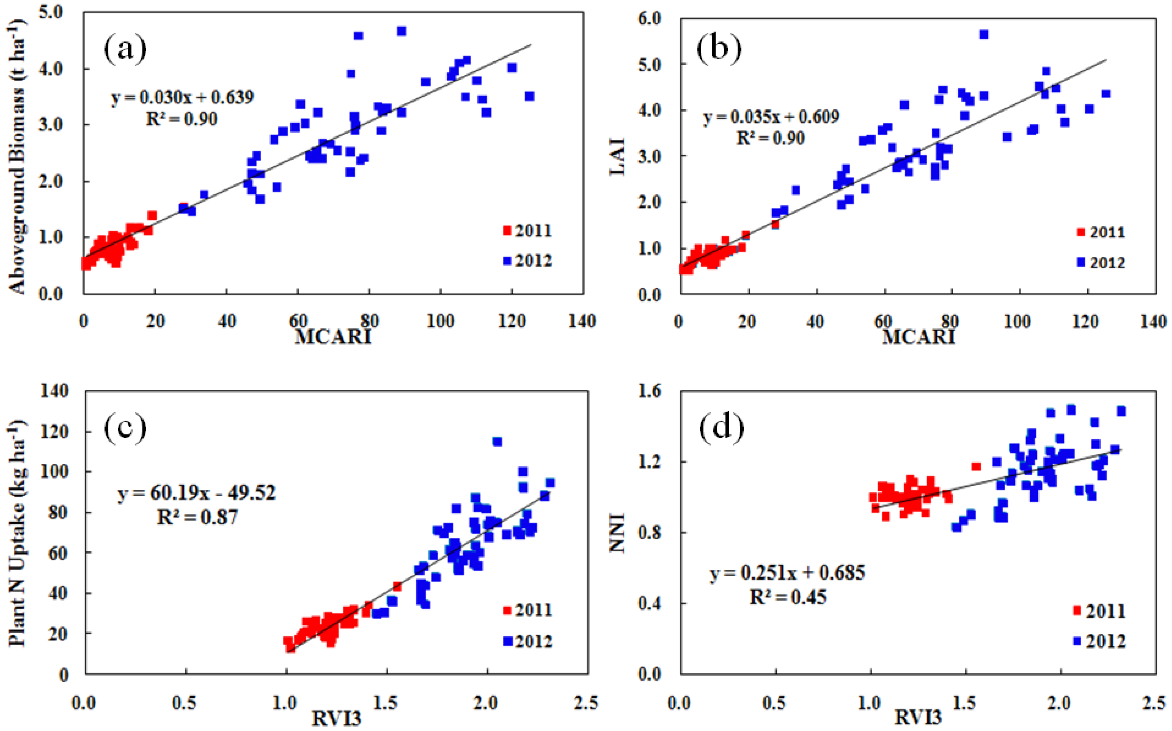
3.2. Vegetation Index Analysis

The performance of the VIs differed with N status indicators. The top 10 VIs for estimating different N status indicators in each year are listed in Table 5.
For aboveground biomass, the top 10 VIs performed similarly in 2011 (R2 = 0.63–0.67) and 2012 (R2 = 0.63–0.64). This was also true for PNU for both years. For LAI, the top 10 VIs performed slightly better in 2011 (R2 = 0.63–0.67) than in 2012 (R2 = 0.58–0.60). Four VIs that are based on the combinations of NIR and red bands, including Ratio Vegetation Index 3 (RVI3), Wide Dynamic Range Vegetation Index 1 (WDRVI1), Soil Adjusted Vegetation Index (SAVI) and Modified Simple Ratio (MSR), were consistently among the top 10 indices for biomass, PNU and LAI. The MCARI index, based on the combination of NIR, red and green bands, had the highest correlation with aboveground biomass (R2 = 0.67) and LAI (R2 = 0.67) in 2011. Four VIs, which included MCARI1, Triangular Vegetation Index (TVI), Modified TVI1 (MTVI1) and Transformed Chlorophyll Absorption in Reflectance Index (TCARI), were also among the top 10 indices for both aboveground biomass and PNU.
Table 5. The top 10 coefficients of determination (R2) for the relationships between vegetation indices based on the FORMOSAT-2 satellite images and rice N status indicators in Heilongjiang Province, China, 2011–2012. Only significant R2 values are listed.
Index201120122011 + 2012Index201120122011 + 2012
Aboveground Biomass (t·ha−1)LAI
MCARI0.67 **0.62 **0.90 **MCARI0.67 **0.58 **0.90 **
DVI30.65 **0.63 **0.90 **DVI20.67 **0.58 **0.91 **
TVI0.64 **0.64 **0.90 **RVI30.65 **0.60 **0.90 **
RVI30.64 **0.63 **0.90 **DVI30.65 **0.60 **0.91 **
MTVI10.63 **0.64 **0.90 **RDVI20.65 **0.58 **0.90 **
MCARI10.63 **0.64 **0.90 **WDRVI10.65 **0.60 **0.90 **
TCARI0.63 **0.64 **0.89 **MSR0.65 **0.60 **0.90 **
WDRVI10.63 **0.64 **0.89 **RDVI30.64 **0.60 **0.90 **
MSR0.63 **0.64 **0.90 **SAVI0.63 **0.61 **0.88 **
SAVI0.61 **0.64 **0.87 **NDVI10.63 **0.61 **0.88 **
Plant N Concentration (%)SPAD Values
DVI4 0.55 **TCI0.27 **0.17 **0.13 **
RDVI4 0.53 **PSRI0.19 ** 0.10 **
NDVI4 0.49 **MTVI20.18 **0.22 **0.16 **
RDVI2 0.49 **TCARI0.16 **0.22 **0.14 **
RVI4 0.49 **MCARI20.15 *0.23 **0.15 **
MGSAVI 0.48 **WDRVI10.14 *0.20 **0.12 **
NDVI2 0.48 **MTVI30.10 *0.25 **0.13 **
GOSAVI 0.48 **TCARI/OSAVI 0.14 **
WDRVI2 0.47 **EVI 0.14 **
mNDVI1 0.30 **DVI0.13* 0.19
Plant N Uptake (kg·ha−1)NNI
RVI30.66 **0.61 **0.87 **RDVI10.18 **0.32 **0.41 **
TVI0.66 **0.61 **0.87 **DVI20.17 **0.33 **0.43 **
WDRVI10.66 **0.62 **0.87 **RVI20.17 **0.33 **0.44 **
RDVI30.66 **0.62 **0.87 **WDRVI20.16 **0.34 **0.43 **
TCARI0.65 **0.63 **0.86 **DVI30.16 **0.34 **0.43 **
MSR0.65 **0.62 **0.87 **RDVI20.16 **0.34 **0.42 **
MCARI10.65 **0.62 **0.87 **RVI30.16 **0.34 **0.45 **
MTVI10.65 **0.62 **0.87 **WDRVI10.15 *0.35 **0.44 **
SAVI0.64 **0.62 **0.85 **RDVI30.15 *0.35 **0.43 **
OSAVI0.64 **0.62 **0.85 **TVI0.15 *0.34 **0.44 **
** Correlation is significant at the 0.01 level; * Correlation is significant at the 0.05 level.
Lower correlations were found between the VIs and NNIs, with R2 of 0.15–0.18 in 2011 and 0.33–0.35 in 2012 for the 10 best models. None of the VIs was significantly correlated with PNC in a specific year, although 30–55% of the PNC variability was explained across the two years (Table 5). The relationships between VIs and SPAD values were also weak, with R2 being 0.10–0.27 and 0.14–0.23 in 2011 and 2012, respectively.
Figure 1. Selected VI regression vs. rice aboveground biomass (a) LAI; (b) plant N uptake (PNU); (c) and NNI; (d) Heilongjiang Province, China, 2011–2012.
Remotesensing 07 10646 g001
Figure 1 shows selected VI models with the best performance in estimating rice aboveground biomass, LAI, PNU and NNI across years. The values for 2011 samples were all smaller than those of 2012. Most samples in 2011 had NNI values close to optimum, and the variability was very small, with CV being only 5%. As a result, a cluster was formed at the lower end of Figure 1d. This may explain why the relationships between VIs and NNI were quite weak in 2011 (Table 5).

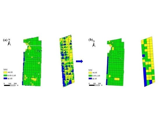
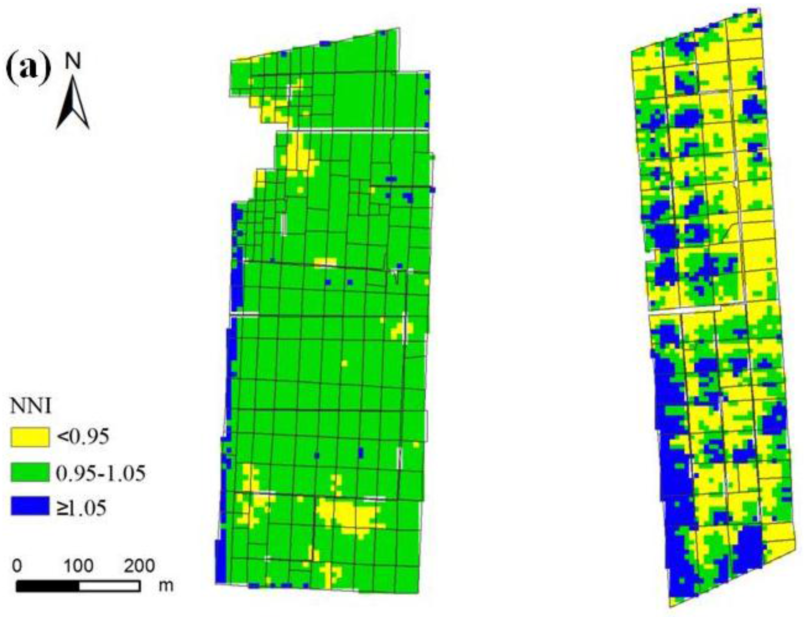
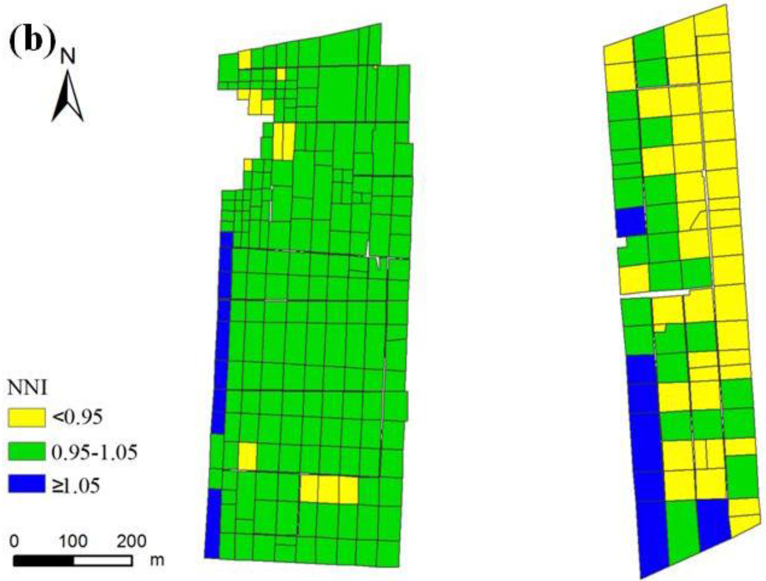
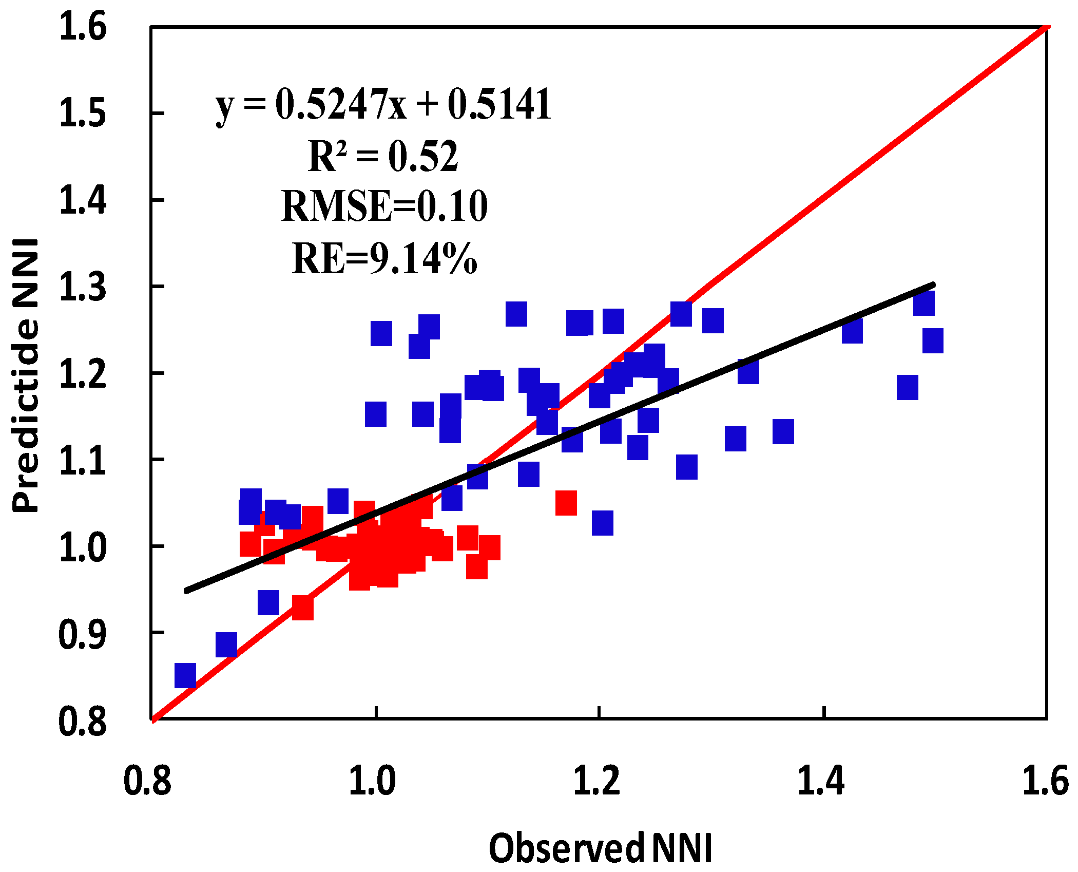
3.3. Nitrogen Status Diagnosis

According to the above results, an indirect NNI estimation method was used in this study. The NNI values estimated this way were moderately correlated with measured NNI across 2011 and 2012 (R2 = 0.52, RMSE = 0.10 and RE = 9.14%) (Figure 2). By comparing the regression line to the 1:1 line in Figure 2, a systematic bias can be identified in the regression model. In particular, when the observed NNI was less than 1.08, the model overestimated the NNI, while the opposite was true when the NNI was greater than 1.08.
The NNI maps created using the indirect method for two farmers’ fields are shown in Figure 3 as an example. Figure 3a,b shows the NNI maps at the pixel level and the plot level, respectively. The first (Figure 3, left) is a well-managed field, with 92% of the field being in the optimal N status category. In contrast, the second field (Figure 3, right) had only 35% in the optimal N category and about 51% in the deficient N category.
A more quantitative and preferable approach is to produce a PNU difference map ( P NU) by subtracting the critical PNU map from the predicted PNU map. This PNU map can not only tell us if the N status is deficient, optimal or surplus, but also the amount of deficiency or surplus. This further can be used to produce a prescription map for topdressing N application rates (NR) at the stem elongation stage. Specifically, the prescription map will be the planned topdressing panicle NR map based on regional best management practice minus the   PNU map. Figure 4 displays a PNU map of the second field shown in Figure 3. About 12% of the field had an N surplus of over 5 kg·ha−1, while 20% of the field had an N deficiency of over 5 kg·ha−1.
Figure 2. Relationship between observed and predicted NNI using MCARI-estimated biomass and RVI3-estimated plant N uptake in 2011 and 2012, Heilongjiang Province, China. The red line is the 1:1 line.
Remotesensing 07 10646 g002
Figure 3. Examples of predicted rice nitrogen nutrition index (NNI) maps of two fields at the pixel level (a) and the plot-level (b), Heilongjiang Province, China.
Remotesensing 07 10646 g003aRemotesensing 07 10646 g003b
Figure 4. Example of a plant N uptake difference map of a farmer’s field, Heilongjiang Province, China.
Remotesensing 07 10646 g004

4. Discussion

4.1. Direct Estimation of NNI

Using satellite remote sensing to estimate rice plant NNI for diagnosing rice N status and guiding in-season site-specific N management across large areas is an attractive idea. How well can we estimate NNI directly using FORMOSAT-2 satellite data? The results of this study indicated that all of the top 10 VIs were significantly correlated with NNI, explaining 18% and 35% of the NNI variability in 2011 and 2012, respectively. Across years, 45% of NNI variability was explained with RVI3. This result is slightly better than what Yao et al. [13] found using the handheld GreenSeeker NDVI and RVI, which explained 25% and 34% of rice NNI variability at the stem elongation stage, respectively. It was found that the top 10 VIs obtained with the three-band Crop Circle ACS 470 sensor explained 61%–69% of rice NNI variability across the panicle initiation and stem elongation stages [12]. However, our study only used data from the panicle initiation stage in 2011, which was expected to be more influenced by the water background than the stem elongation stage. In general, it is not satisfactory to use satellite images to directly estimate rice plant NNI at this stage. At later stages when the rice plants reach canopy closure, this approach may work better. However, it may then be too late for guiding in-season N application.

4.2. Indirect Estimation of NNI

An alternative approach is to use remote sensing to estimate key parameters and indirectly estimate NNI. Cilia et al. [24] used aerial hyperspectral remote sensing to estimate maize N concentration and biomass and then estimated NNI indirectly. Our study indicated that biomass could be reliably estimated using satellite remote sensing at the panicle initiation and stem elongation stages, with over 60% of its variability being explained by the top 10 VIs in both 2011 and 2012. We selected MCARI for further analysis. This index was initially developed for estimating leaf chlorophyll variation, but it was also significantly related to LAI [54,55]. In this study, the MCARI index was highly correlated with rice aboveground biomass and LAI (R2 = 0.58–0.67). The results agree with those of Cao et al. [12], who also identified a modified MCARI as the best index for estimating rice biomass (R2 = 0.79) and plant N uptake (R2 = 0.83) across growth stages. The top 10 Crop Circle VIs in their study explained 50%–54% of rice biomass variability across the panicle initiation and stem elongation stages. Our results were comparable to the results (R2 = 0.68–0.69) of Gnyp et al. [61] that were obtained with optimized narrow band RVI and NDVI for estimating rice biomass at the stem elongation stage. However, estimating rice PNC before canopy closure is a great challenge. We did not find any significant correlation between VIs and rice PNC in this study. This was also stated by Yao et al. [13]. They found that the GreenSeeker NDVI and RVI were not significantly correlated with rice PNC at the stem elongation stage. Cao et al. [12] found that the three-band Crop Circle ACS 470 sensor at best explained 33% of rice PNC across the panicle initiation and stem elongation stages using the Red Edge Green Difference Vegetation Index (REGDVI). Even with hyperspectral remote sensing, Yu et al. [62] only explained 39% of rice PNC variability across the tillering and heading stages using the Optimized Simple Ratio or Normalized Difference Index. Before canopy closure, soil and water backgrounds in paddy rice fields can influence plant reflectance [63]. In addition, plant biomass dominates canopy reflectance before the heading stage, making the estimation of chlorophyll and N concentration at early growth stages difficult [20]. Therefore, the approach adopted by Cilia et al. [24] did not work for rice monitoring at the panicle initiation and stem elongation stages in our study.
A practical approach is to use satellite remote sensing to estimate rice biomass and PNU. From the estimated biomass and the critical N dilution curve, the critical PNU can be determined, and NNI will be calculated using the estimated PNU and the critical PNU. The results of this study supported this idea. Over 60% of rice PNU variability was explained by RVI3 in both years. This was even better than the result obtained with the GreenSeeker sensor for estimating rice PNU at the stem elongation stage (R2 = 0.40–0.41) by Yao et al. [13] and similar to the results (R2 = 0.63–0.65) obtained with the Crop Circle ACS 470 sensor for estimating rice PNU across the panicle initiation and stem elongation stages by Cao et al. [12]. The estimated NNI obtained this way explained 52% of the measured NNI variability across 2011 and 2012, which was slightly better than the direct estimation of NNI using VIs obtained from satellite images (R2 = 0.45).

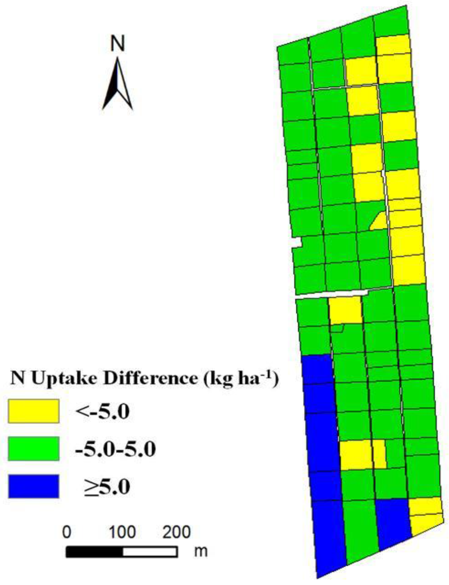
4.3. Applications for Rice N Status Diagnosis and Topdressing N Recommendation

After the NNI map is generated, it is necessary to define the NNI thresholds for N status diagnosis. The current thresholds (NNI < 1: deficient; NNI = 1: optimal; NNI > 1: surplus) may need to be further refined for practical applications. For example, the NNI values of 0.99 and 1.01 are very close to each other and are all quite optimal, but they will be classified as deficient and surplus N status, respectively, based on current thresholds. Cilia et al. [24] proposed to classify NNI into five classes (NNI ≤ 0.7, 0.7 < NNI ≤ 0.9, 0.9 < NNI ≤ 1.1, 1.1 < NNI ≤ 1.3, NNI > 1.3) and regarded NNI ≤ 0.9 as N deficient, 0.9 < NNI ≤ 1.1 as N optimal and NNI > 1.1 as N surplus. Based on the rice N management situations in the study region, we proposed the following thresholds for rice: NNI ≤ 0.95 as N deficient, 0.95 < NNI ≤ 1.05 as N optimal and NNI > 1.05 as N surplus. These threshold values can be used to delineate a field into three regions with different N nutritional status. The diagnosis results shown in Figure 3 indicated that the first field (Figure 3 left) was well managed, with the majority of the field having an optimal N status, while about 51% of the second field (Figure 3, right) was deficient in N. These agreed quite well with the two farmers’ management practices. However, these threshold values are empirical, and more studies are needed to further test and refine these thresholds by relating NNI to relative grain yield.
The NNI-based rice N status map can be used to guide in-season topdressing N application. For the optimal N zone, 30 kg·N·ha−1 was recommended based on the regional best N management practice. For the deficient N zone, 35 or 40 kg·ha−1 can be recommended, and for the surplus N zone 25 or 20 kg·ha−1. This approach is commonly used in site-specific N management of rice based on CM diagnosis developed by the International Rice Research Institute [64]. It is empirical, but very practical for on-farm applications in small-scale farming areas of Asia. A more quantitative approach is to produce a PNU difference map using the estimated PNU map minus the critical PNU map. The recommended N topdressing application rate can be determined using the regional optimum topdressing N application rate minus the PNU difference. This approach is different from the variable rate N application strategy proposed by Cilia et al. [24]. They first computed the average PNU from the optimal NNI pixels and then used this average value together with the estimated PNU to calculate the difference, and for N deficient pixels, the deficient amounts were used as variable N application rates. For pixels with optimal and surplus N, no N fertilizers were recommended. In our approach, we did not analyze the pixel scale, because in rice farming, the field is divided into many small plots for irrigation purpose. These plots also serve as management units. We applied plot-average NNI values to diagnose the rice N status of each plot. Our precision N management strategy takes the regional optimal N rate as the initial total N rate, with 40% and 30% being applied as basal and tillering N fertilizers, respectively. For topdressing N application at the stem elongation stage, 30% of the initial total N rate should be applied if the N status is optimal. Otherwise, the topdressing N rates can be adjusted based on deficient or surplus N amounts. Even if the N status is optimal at the stem elongation stage, it only indicates the N status at that stage, which is more than two months prior to harvest, and a certain amount of N fertilizers should still be recommended to meet the N requirements from stem elongation to harvest.

4.4. Challenges and Future Research Needs

The proposed approach discussed above requires the satellite imagery to be collected in a narrow time window, preferably one week before topdressing N application at the stem elongation stage for rice in the study region. If the image is collected too early, the diagnosis result may not match the true rice N status at the stem elongation stage. In addition, rice plants will be too small, and the water background will strongly influence the plant reflectance. If the image is collected too close to the stem elongation stage, it may be too late to use the diagnosis result for guiding the topdressing N application. Therefore, a satellite with a high temporal resolution is required. The daily revisit time of the FORMOSAT-2 satellite makes it ideal for this purpose. Its 8-m spatial resolution may be too coarse for small-scale farming in other parts of China, such as in the North China Plain [65], but is good enough for large-scale farming in the Sanjiang Plain of Northeast China.
It should be noted that there are 7–10 days between the panicle initiation and stem elongation stages, and the rice plants are fast developing, so the rice biomass and plant N uptake determined at the panicle initiation stage are smaller than the values at the stem elongation stage. Studies are needed to determine the influence of this difference on the recommended topdressing N application rates.
Year to year weather variability poses a challenge to use satellite remote sensing for in-season rice N status diagnosis and guiding topdressing application. The satellite imageries were collected at similar times in both years. However, the temperature in 2012 was higher than 2011. The accumulated temperature from transplanting date to the sampling date of 2012 was about 100 °C higher than that in 2011. As a result, rice plants grew faster in 2012 and already reached the stem elongation stage when the image was collected on 26 June 2012. This was reflected by the larger biomass, LAI and plant N uptake values in 2012 than 2011 (Table 3). Another factor to consider is that there are many cloudy and rainy days during the growing season in many parts of the major rice planting regions, which can prevent us from getting the needed satellite images within the narrow time window [13] in some years. Such uncertainty in year to year weather variability makes it very difficult to collect the satellite images at the right time for guiding in-season N management.
To overcome this limitation, multi-temporal and dual-polarimetric TerraSAR-X satellite data were evaluated for monitoring rice crop growth, and very promising results were obtained for rice biomass estimation [66]. Low-altitude remote sensing based on unmanned aerial vehicles (UAVs) may also be an alternative way for diagnosing in-season rice N status and guiding variable rate N management [67,68,69]. Due to the quick turn-around time, UAV-based remote sensing images can be collected 1–2 days before the topdressing N application, and the diagnosis result will be more representative. Nevertheless, due to the much smaller coverage and bigger data volume of UAV images, they are still not very practical for regional studies over large areas.
The FORMOSAT-2 satellite images only have four commonly-used wavebands (B, G, R and NIR). Previous research indicated that red edge-based vegetation indices performed better for estimating crop N status NNI than traditional red light-based indices [7,12,70]. According to Li et al. [70], the red edge-based Canopy Chlorophyll Content Index (CCCI) was reported to have the best performance among all of the indices evaluated for estimating summer maize N concentration and uptake at V6, V7 and V10–V12 stages, based on the simulation of Crop Circle ACS 470 active sensor, RapidEye and WorldView 2 satellite images. It is necessary to evaluate the potential improvements in estimating rice NNI using RapidEye and WorldView 2 satellite images. Hyperspectral sensing has the potential to further improve the estimation of crop NNI, as demonstrated in winter wheat [20] and summer maize [21], and more studies are needed to explore the potential of hyperspectral sensing for monitoring crop NNI.
In summary, the proposed satellite remote sensing approach can achieve comparable performance as ground-based active canopy sensors for estimating rice N status and is applicable to other rice planting regions. It is more efficient for large area applications, but is more influenced by weather conditions, while active canopy sensors are independent of environmental light conditions. It requires special training to process satellite remote sensing data, while active canopy sensors are easy to use, but are not suitable for large area applications. The UAV-based approach, coupled with red edge-based indices and hyperspectral remote sensing, has the potential to overcome the disadvantages of the ground active sensing and satellite remote sensing approaches. Therefore, it deserves further studies.

5. Conclusions

This study evaluated the potential of using FORMOSAT-2 satellite images to estimate rice NNI at the panicle initiation stage for guiding topdressing N application at the stem elongation stage in Northeast China. Across years, 45% of NNI variability could be explained using the RVI3 index directly. On the other hand, the indirect approach using FORMOSAT-2 images to estimate the aboveground biomass, PNU and, consequently, NNI achieved slightly better results (R2 = 0.52 across years). Moreover, the calculated difference between the estimated PNU and the critical PNU based on the indirect method can be used to guide the topdressing N application rate adjustments, which demonstrated that FORMOSAT-2 images have the potential to estimate rice N status for guiding panicle N fertilizer applications in Northeast China. However, more studies are needed to further evaluate and improve the proposed method of in-season rice N status diagnosis and precision N management strategy under different on-farm conditions using different types of satellite data. The potential of UAV-based remote sensing, coupled with red edge-based indices and hyperspectral sensors, for improving rice NNI monitoring also needs to be studied in future research.

Acknowledgements

This study was financially supported by the National Basic Research Program (2015CB150405), the Natural Science Foundation of China (31071859), the Innovative Group Grant of the Natural Science Foundation of China (31421092), the European Aeronautic Defense and Space Company (EADS), the CHN-2152, 14-0039 SINOGRAIN project and the Sino-UK Newton AgriTech Remote Sensing for Sustainable Intensification project. We thank the staff of the Jiansanjiang Bureau of Agricultural Land Reclamation, Qixing Farm, and the Jiansanjiang Institute of Agricultural Sciences for their support. We also would like to thank all of the farmers for their cooperation in this research, and Prasad Thenkabail, Tao Cheng and the anonymous reviewers for their suggestions to improve the manuscript.

Author Contributions

Yuxin Miao and Georg Bareth conceived and guided the study. Shanyu Huang, Guangming Zhao, Xiaobo Ma, Chuanxiang Tan, Weifeng Yu and Martin L. Gnyp conducted the field experiments. Shanyu Huang performed the image processing and data analysis, Yuxin Miao and Shanyu Huang wrote the paper, Georg Bareth, Fei Yuan, Victoria I.S. Lenz-Wiedemann, Martin L. Gnyp and Uwe Rascher provided suggestions for the study, reviewed and edited the manuscript. All authors read and approved the manuscript.

Conflicts of Interest

The authors declare no conflict of interest.

References

  1. Dawe, D. The contribution of rice research to poverty alleviation. Stud. Plant Sci. 2000, 7, 3–12. [Google Scholar]
  2. Zhang, F.; Cui, Z.; Fan, M.; Zhang, W.; Chen, X.; Jiang, R. Integrated soil-crop system management: Reducing environmental risk while increasing crop productivity and improving nutrient use efficiency in China. J. Environ. Qual. 2011, 40, 1051–1057. [Google Scholar] [CrossRef] [PubMed]
  3. Zhang, F.; Wang, J.; Zhang, W.; Cui, Z.; Ma, W.; Chen, X.; Jiang, R. Nutrient use efficiencies of major cereal crops in China and measures for improvement. Acta Pedolog. Sin. 2008, 5, 915–924. [Google Scholar]
  4. Jin, J. Changes in the efficiency of fertiliser use in China. J. Sci. Food Agric. 2012, 92, 1006–1009. [Google Scholar] [CrossRef] [PubMed]
  5. Ju, X.; Xing, G.; Chen, X.; Zhang, S.; Zhang, L.; Liu, X.; Cui, Z.; Yin, B.; Christie, P.; Zhu, Z.; et al. Reducing environmental risk by improving N management in intensive Chinese agricultural systems. Proc. Natl. Acad. Sci. USA. 2009, 106, 3041–3046. [Google Scholar] [CrossRef] [PubMed] [Green Version]
  6. Doberman, A.; Witt, C.; Dawe, D.; Abdulrachman, S.; Gines, H.C.; Nagarajan, R.; Satawathananont, S.; Son, T.T.; Tan, P.S.; Wang, G.H.; et al. Site-specific nutrient management for intensive rice cropping systems in Asia. Field Crops Res. 2002, 74, 37–66. [Google Scholar] [CrossRef]
  7. Cao, Q.; Miao, Y.; Feng, G.; Gao, X.; Li, F.; Liu, B.; Yue, S.; Cheng, S.; Ustin, S.; Khosla, R. Active canopy sensing of winter wheat nitrogen status: An evaluation of two sensor systems. Comput. Electron. Agric. 2015, 112, 54–67. [Google Scholar] [CrossRef]
  8. Greenwood, D.J.; Neeteson, J.J.; Draycott, A. Quantitative relationships for the dependence of growth rate of arable crops on their nitrogen content, dry weight and aerial environment. Plant Soil 1986, 91, 281–301. [Google Scholar] [CrossRef]
  9. Greenwood, D.J.; Gastal, F.; Lemaire, G.; Draycott, A.; Millard, P.; Neeteson, J.J. Growth rate and % N of field grown crops: Theory and experiments. Ann. Bot. 1991, 67, 181–190. [Google Scholar]
  10. Lemaire, G.; Jeuffroy, M.H.; Gastal, F. Diagnosis tool for plant and crop N status in vegetative stage: Theory and practices for crop N management. Eur. J. Agron. 2008, 28, 614–624. [Google Scholar] [CrossRef]
  11. Houlès, V.; Guerif, M.; Mary, B. Elaboration of a nitrogen nutrition indicator for winter wheat based on leaf area index and chlorophyll content for making nitrogen recommendations. Eur. J. Agron. 2007, 27, 1–11. [Google Scholar] [CrossRef]
  12. Cao, Q.; Miao, Y.; Wang, H.; Huang, S.; Cheng, S.; Khosla, R.; Jiang, R. Non-destructive estimation of rice plant nitrogen status with crop circle multispectral active canopy sensor. Field Crops Res. 2013, 154, 133–144. [Google Scholar] [CrossRef]
  13. Yao, Y.; Miao, Y.; Cao, Q.; Wang, H.; Gnyp, M.L.; Bareth, G.; Khosla, R.; Yang, W.; Liu, F.; Liu, C. In-season estimation of rice nitrogen status with an active crop canopy sensor. IEEE J. Sel. Topics Appl. Earth Observ. Remote Sens. 2014, 7, 4403–4413. [Google Scholar] [CrossRef]
  14. Debaeke, P.; Rouet, P.; Justes, E. Relationship between the normalized SPAD index and the nitrogen nutrition index: Application to durum wheat. J. Plant Nutr. 2006, 29, 75–92. [Google Scholar] [CrossRef]
  15. Prost, L.; Jeuffroy, M.H. Replacing the nitrogen nutrition index by the chlorophyll meter to assess wheat N status. Agron. Sustain. Dev. 2007, 27, 321–330. [Google Scholar] [CrossRef]
  16. Ziadi, N.; Bélanger, G.; Claessens, A.; Lefebvre, L.; Tremblay, N.; Cambouris, A.N.; Nolin, M.C.; Parent, L.É. Plant-based diagnostic tools for evaluating wheat nitrogen status. Crop Sci. 2010, 50, 2580–2590. [Google Scholar] [CrossRef]
  17. Cao, Q.; Cui, Z.; Chen, X.; Khosla, R.; Dao, T.H.; Miao, Y. Quantifying spatial variability of indigeneous nitrogen supply for precision nitrogen management in small sacle farming. Precis. Agric. 2012, 13, 45–61. [Google Scholar] [CrossRef]
  18. Ziadi, N.; Brassard, M.; Bélanger, G.; Claessens, A.; Tremblay, N.; Cambouris, A.N.; Nolin, M.C.; Parent, L.-É. Chlorophyll measurements and nitrogen nutrition index for the evaluation of corn nitrogen status. Agron. J. 2008, 100, 1264–1273. [Google Scholar] [CrossRef]
  19. Miao, Y.; Mulla, D.J.; Randall, G.W.; Vetsch, J.A.; Vintila, R. Combining chlorophyll meter readings and high spatial resolution remote sensing images for in-season site-specific nitrogen management of corn. Precis. Agric. 2009, 10, 45–62. [Google Scholar] [CrossRef]
  20. Mistele, B.; Schmidhalter, U. Estimating the nitrogen nutrition index using spectral canopy reflectance measurements. Eur. J. Agron. 2008, 29, 184–190. [Google Scholar] [CrossRef]
  21. Chen, P.; Wang, J.; Huang, W.; Tremblay, N.; Ouyang, Z.; Zhang, Q. Critical nitrogen curve and remote detection of nitrogen nutrition index for corn in the Northwestern Plain of Shandong Province, China. IEEE J. Sel. Topics Appl. Earth Observ. Remote Sens. 2013, 6, 682–689. [Google Scholar] [CrossRef]
  22. Holland, K.H.; Lamb, D.W.; Schepers, J.S. Radiometry of proximal active optical sensors (AOS) for agricultural sensing. IEEE J. Sel. Topics Appl. Earth Observ. Remote Sens. 2012, 5, 1793–1802. [Google Scholar] [CrossRef]
  23. Mulla, D.J. Twenty five years of remote sensing in precision agriculture: Key advances and remaining knowledge gaps. Biosyst. Eng. 2013, 114, 358–371. [Google Scholar] [CrossRef]
  24. Cilia, C.; Panigada, C.; Rossini, M.; Meroni, M.; Busetto, L.; Amaducci, S.; Boschetti, M.; Picchi, V.; Colombo, R. Nitrogen status assessment for variable rate fertilization in maize through hyperspectral imagery. Remote Sens. 2014, 6, 6549–6565. [Google Scholar] [CrossRef] [Green Version]
  25. Wu, J.; Wang, D.; Rosen, C.J.; Bauer, M.E. Comparison of petiole nitrate concentrations, SPAD chlorophyll readings, and QuickBird satellite imagery in detecting nitrogen status of potato canopies. Field Crops Res. 2007, 101, 96–103. [Google Scholar] [CrossRef]
  26. Yang, C.M.; Liu, C.C.; Wang, Y.W. Using FORMOSAT-2 satellite data to estimate leaf area index of rice crop. J. Photogram. Remote Sens. 2008, 13, 253–260. [Google Scholar]
  27. Darvishzadeh, R.; Matkan, A.A.; Ahangar, A.D. Inversion of a radiative transfer model for estimation of rice canopy chlorophyll content using a lookup-table approach. IEEE J. Sel. Topics Appl. Earth Observ. Remote Sens. 2012, 5, 1222–1230. [Google Scholar] [CrossRef]
  28. Xing, B.; Dudas, M.J.; Zhang, Z.; Qi, X. Pedogenetic characteristics of albic soils in the three river plain, Heilongjiang Province. Acta Pedolog. Sin. 1994, 31, 95–104. [Google Scholar]
  29. Wang, Y.; Yang, Y. Effects of agriculture reclamation on hydrologic characteristics in the Sanjiang Plain. Chin. Geogr. Sci. 2001, 11, 163–167. [Google Scholar] [CrossRef]
  30. Yan, M.; Deng, W.; Chen, P. Climate change in the Sanjiang Plain disturbed by large-scale reclamation. J. Geogr. Sci. 2002, 12, 405–412. [Google Scholar]
  31. Yao, Y.; Miao, Y.; Huang, S.; Gao, L.; Zhao, G.; Jiang, R.; Chen, X.; Zhang, F.; Yu, K.; et al. Active canopy sensor-based precision N management strategy for rice. Agron. Sustain. Dev. 2012, 32, 925–933. [Google Scholar] [CrossRef]
  32. Zhao, G.; Miao, Y.; Wang, H.; Su, M.; Fan, M.; Zhang, F.; Jiang, R.; Zhang, Z.; Liu, C.; Liu, P.; et al. A preliminary precision rice management system for increasing both grain yield and nitrogen use efficiency. Field Crops Res. 2013, 154, 23–30. [Google Scholar] [CrossRef]
  33. Chern, J.S.; Wu, A.M.; Lin, S.F. Lesson learned from FORMOSAT-2 mission operations. Acta Astronaut. 2006, 59, 344–350. [Google Scholar] [CrossRef]
  34. Liu, C.C. Processing of FORMOSAT-2 daily revisit imagery for site surveillance. IEEE Trans. Geosci. Remote Sens. 2006, 44, 3206–3214. [Google Scholar] [CrossRef]
  35. Bei, J.H.; Wang, K.R.; Chu, Z.D.; Chen, B.; Li, S.K. Comparitive study on the measurement methods of the leaf area. J. Shihezi Uni. 2005, 23, 216–218. [Google Scholar]
  36. Lv, W.; Ge, Y.; Wu, J.; Chang, J. Study on the method for the determination of nitric nitrogen, ammoniacal nitrogen and total nitrogen in plant. Spectrosc. Spect. Anal. 2004, 24, 204–206. [Google Scholar]
  37. Li, N. The comparison on various methods for determing different proteins. J. Shanxi Agric. Univ. 2006, 26, 132–134. [Google Scholar]
  38. Justes, E.; Mary, B.; Meynard, J.M.; Machet, J.M.; Thelier-Huche, L. Determination of a critical nitrogen dilution curve for winter wheat crops. Ann. Bot. 1994, 74, 397–407. [Google Scholar] [CrossRef]
  39. Tucker, C.J. Red and photographic infrared linear combinations for monitoring vegetation. Remote Sens. Environ. 1979, 8, 127–150. [Google Scholar] [CrossRef]
  40. Buschmann, C.; Nagel, E. In vivo spectroscopy and internal optics of leaves as basis for remote sensing of vegetation. Int. J. Remote Sens. 1993, 14, 711–722. [Google Scholar] [CrossRef]
  41. Gitelson, A.A.; Kaufman, Y.J.; Merzlyak, M.N. Use of a green channel in remote sensing of global vegetation from EOS-MODIS. Remote Sens. Environ. 1996, 58, 289–298. [Google Scholar] [CrossRef]
  42. Roujean, J.L.; Breon, F.M. Estimating PAR absorbed by vegetation from bidirectional reflectance measurements. Remote Sens. Environ. 1995, 51, 375–384. [Google Scholar] [CrossRef]
  43. Gitelson, A.A.; Gritz, Y.; Merzlyak, M.N. Relationships between leaf chlorophyll content and spectral reflectance and algorithms for non-destructive chlorophyll assessment in higher plant leaves. J. Plant Physiol. 2003, 160, 271–282. [Google Scholar] [CrossRef] [PubMed]
  44. Gitelson, A.A. Wide dynamic range vegetation index for remote quantification of biophysical characteristics of vegetation. J. Plant Physiol. 2004, 161, 165–173. [Google Scholar] [CrossRef] [PubMed]
  45. Huete, A.R. A soil-adjusted vegetation index (SAVI). Remote Sens. Environ. 1988, 25, 295–309. [Google Scholar] [CrossRef]
  46. Chen, J.M. Evaluation of vegetation indices and a modified simple ratio for boreal applications. Can. J. Remote Sens. 1996, 22, 229–242. [Google Scholar] [CrossRef]
  47. Rondeaux, G.; Steven, M.; Baret, F. Optimization of soil-adjusted vegetation indices. Remote Sens. Environ. 1996, 55, 95–107. [Google Scholar] [CrossRef]
  48. Qi, J.; Chehbouni, A.; Huete, A.R.; Kerr, Y.H.; Sorooshian, S. A modified soil adjusted vegetation index. Remote Sens. Environ. 1994, 48, 119–126. [Google Scholar] [CrossRef]
  49. Datt, B. Visible/near infrared reflectance and chlorophyll content in Eucalyptus leaves. Int. J. Remote Sens. 1999, 20, 2741–2759. [Google Scholar] [CrossRef]
  50. Wang, W.; Yao, X.; Yao, X.F.; Tian, Y.C.; Liu, X.J.; Ni, J.; Cao, W.X.; Zhu, Y. Estimating leaf nitrogen concentration with three-band vegetation indices in rice and wheat. Field Crops Res. 2012, 129, 90–98. [Google Scholar] [CrossRef]
  51. Sims, D.A.; Gamon, J.A. Relationships between leaf pigment content and spectral reflectance across a wide range of species, leaf structures and developmental stage. Remote Sens. Environ. 2002, 81, 337–354. [Google Scholar] [CrossRef]
  52. Gitelson, A.A.; Kaufman, Y.J.; Stark, R.; Rundquist, D. Novel algorithms for remote estimation of vegetation fraction. Remote Sens. Environ. 2002, 80, 76–87. [Google Scholar] [CrossRef]
  53. Peñuelas, J.; Baret, F.; Filella, I. Semi-empirical indices to assess carotenoids/chlorophyll a ratio from leaf spectral reflectance. Photosynthetica. 1995, 32, 221–230. [Google Scholar]
  54. Daughtry, C.S.T.; Walthall, C.L.; Kim, M.S.; Colstoun, E.B.; McMurtrey, J.E., III. Estimating corn leaf chlorophyll concentration from leaf and canopy reflectance. Remote Sens. Environ. 2000, 74, 229–239. [Google Scholar] [CrossRef]
  55. Haboudane, D.; Miller, J.R.; Pattey, E.; Zarco-Tejada, P.J.; Strachan, I.B. Hyperspectral vegetation indices and novel algorithms for predicting green LAI of crop canopies: Modeling and validation in the context of precision agriculture. Remote Sens. Environ. 2004, 90, 337–352. [Google Scholar] [CrossRef]
  56. Haboudane, D.; Miller, J.R.; Tremblay, N.; Zarco-Tejada, P.J.; Dextraze, L. Integrated narrow-band vegetation indices for prediction of crop chlorophyll content for application to precision agriculture. Remote Sens. Environ. 2002, 81, 416–426. [Google Scholar] [CrossRef]
  57. Broge, N.H.; Leblanc, E. Comparing prediction power and stability of broadband and hyperspectral vegetation indices for estimation of green leaf area index and canopy chlorophyll density. Remote Sens. Environ. 2000, 76, 156–172. [Google Scholar] [CrossRef]
  58. Huete, A.; Didan, K.; Miura, T.; Rodriguez, E.P.; Gao, X.; Ferreira, L.G. Overview of the radiometric and biophysical performance of the MODIS vegetation indices. Remote Sens. Environ. 2002, 83, 195–213. [Google Scholar] [CrossRef]
  59. Haboudane, D.; Tremblay, N.; Miller, J.R.; Vigneault, P. Remote estimation of crop chlorophyll content using spectral indices derived from hyperspectral data. IEEE Trans.Geosci. Remote. Sens. 2008, 46, 423–437. [Google Scholar] [CrossRef]
  60. Eitel, J.U.H.; Long, D.S.; Gessler, P.E.; Smith, A.M.S. Using in-situ measurements to evaluate the new RapidEye™ satellite series for prediction of wheat nitrogen status. Int. J. Remote Sens. 2007, 28, 4183–4190. [Google Scholar] [CrossRef]
  61. Gnyp, M.L.; Miao, Y.; Yuan, F.; Ustin, S.L.; Yu, K.; Yao, Y.; Huang, S.; Bareth, G. Hyperspectral canopy sensing of paddy rice aboveground biomass at different growth stages. Field Crops Res. 2014, 155, 42–55. [Google Scholar] [CrossRef]
  62. Yu, K.; Li, F.; Gnyp, M.L.; Miao, Y.; Bareth, G.; Chen, X. Remotely detecting canopy nitrogen concentration and uptake of paddy rice in the Northeast China Plain. ISPRS J. Photogramm. Remote Sens. 2013, 78, 102–115. [Google Scholar] [CrossRef]
  63. Van Niel, T.G.; McVicar, T.R. Current and potential uses of optical remote sensing in rice-based irrigation systems: A review. Aust. J. Agric. Res. 2004, 55, 155–185. [Google Scholar] [CrossRef]
  64. Peng, S.; Buresh, R.J.; Huang, J.; Zhong, X.; Zou, Y.; Yang, J.; Wang, G.; Liu, Y.; Hu, R.; Tang, Q.; Cui, K.; Zhang, F.; Dobermann, A. Improving nitrogen fertilization in rice by site-specific N management. A review. Agron. Sustain. Dev. 2010, 30, 649–656. [Google Scholar] [CrossRef]
  65. Shen, J.; Cui, Z.; Miao, Y.; Mi, G.; Zhang, H.; Fan, M.; Zhang, C.; Jiang, R.; Zhang, W.; Li, H.; et al. Transforming agriculture in China: From solely high yield to both high yield and high resource use efficiency. Global Food Sec. 2013, 2, 1–8. [Google Scholar] [CrossRef]
  66. Koppe, W.; Gnyp, M.L.; Hütt, C.; Yao, Y.; Miao, Y.; Chen, X.; Bareth, B. Rice monitoring with multi-temporal and dual-polarimetric TerraSAR-X data. Int. J. Appl. Earth Observ. Geoinf. 2013, 21, 568–576. [Google Scholar] [CrossRef]
  67. Zhang, C.; Kovacs, J.M. The application of small unmanned aerial systems for precision agricuture: A review. Precis. Agric. 2012, 13, 693–712. [Google Scholar] [CrossRef]
  68. Huang, Y.; Thomson, S.J.; Hoffmann, W.C.; Lan, Y.; Fritz, B.K. Development and prospect of unmanned aerial vehicle technologies for agricultural production management. Int. J. Agric. Biol. Eng. 2013, 6, 1–10. [Google Scholar]
  69. Uto, K.; Seki, H.; Saito, G.; Kosugi, Y. Characterization of rice paddies by a UAV-mounted miniature hyperspectral sensor system. IEEE J. Sel. Topics Appl. Earth Observ. Remote Sens. 2013, 6, 851–860. [Google Scholar] [CrossRef]
  70. Li, F.; Miao, Y.; Feng, G.; Yuan, F.; Yue, S.; Gao, X.; Liu, Y.; Liu, B.; Ustin, S.L.; Chen, X. Improving estimation of summer maize nitrogen status with red edge-based spectral vegetation indices. Field Crops Res. 2014, 157, 111–123. [Google Scholar] [CrossRef]

