Article

Extracting the Green Fractional Vegetation Cover from Digital Images Using a Shadow-Resistant Algorithm (SHAR-LABFVC)

The State Key Laboratory of Remote Sensing Science, Beijing Key Laboratory for Remote Sensing of Environment and Digital Cities, School of Geography, Beijing Normal University, Beijing 100875, China
*
Author to whom correspondence should be addressed.
Remote Sens. 2015, 7(8), 10425-10443; https://doi.org/10.3390/rs70810425
Submission received: 10 June 2015 / Accepted: 7 August 2015 / Published: 14 August 2015

Abstract

:
Taking photographs with a commercially available digital camera is an efficient and objective method for determining the green fractional vegetation cover (FVC) for field validation of satellite products. However, classifying leaves under shadows in processing digital images remains challenging and results in classification errors. To address this problem, an automatic shadow-resistant algorithm in the Commission Internationale d’Eclairage L*a*b* color space (SHAR-LABFVC) based on a documented FVC estimation algorithm (LABFVC) is proposed in this paper. The hue saturation intensity (HSI) is introduced in SHAR-LABFVC to enhance the brightness of shaded parts of the image. The lognormal distribution is used to fit the frequency of vegetation greenness and to classify vegetation and the background. Real and synthesized images are used for evaluation, and the results are in good agreement with the visual interpretation, particularly when the FVC is high and the shadows are deep, indicating that SHAR-LABFVC is shadow resistant. Without specific improvements to reduce the shadow effect, the underestimation of FVC can be up to 0.2 in the flourishing period of vegetation at a scale of 10 m. Therefore, the proposed algorithm is expected to improve the validation accuracy of remote sensing products.

Graphical Abstract

1. Introduction

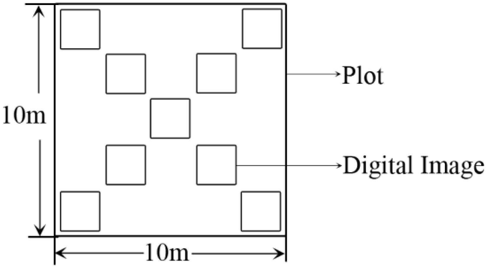
Fractional vegetation cover (FVC) is widely used to describe vegetation quality and ecosystem changes and is a controlling factor in transpiration, photosynthesis and other terrestrial processes [1,2,3]. Estimating FVC in field measurements is critical because it provides a baseline for improving remote sensing algorithms and validating products.
Visual estimation, sampling [4], photography [5] and other techniques are commonly used in field measurements. Among these, photography with digital cameras is one of the most important methods. Analyzing digital images to calculate FVC is efficient and accurate in most circumstances [3,5,6,7,8,9,10,11]. The parts of an image that contain vegetation can be determined based on their physical, shape and color characteristics and other features [6,7,8,12]. In general, these methods can be grouped into two classes: (1) cluster analysis based on training samples, e.g., supervised and unsupervised classifications [13,14] and object-based image analysis methodology (OBIA) [15,16]; and (2) threshold-based methods according to the vegetation index, such as the color index of vegetation extraction (CIVE) [17], the excess green index (ExG) [18,19], excess green minus excess red (ExG−ExR) [20], and many other indices [11,21]. When these two types of methods are used for image classification, different color spaces are usually introduced and analyzed, for example red green blue (RGB) and hue saturation intensity (HSI) color spaces [12], for the mean-shift-based color segmentation method and the Commission Internationale d’Eclairage L*a*b* (LAB) color space for the documented FVC estimation algorithm named LABFVC [22] and LAB2 [23].
However, shadows should be addressed when FVC is extracted from a digital image. Shadows projected by vegetation increase the contrast in an image, alter the color in shaded areas and affect the image analysis. Shadows occur not only on the soil, but also inside the vegetation canopy [15].
Although a series of methods have been proposed, the shadow problem has not been perfectly solved. Visual interpretation using the supervised classification tool via commercial image processing software can perfectly distinguish vegetation in shadows through human to computer interaction. However, this method requires many manual steps and is less automatic and efficient [13,14,16]. Manual steps can cause bias and inconsistency between observers [24]. Methods based on physical characteristics [15,16] and feature space analysis [12] have been proposed to solve the shadow problem, but are time consuming and unsuitable for real-time applications. Using artificial shelters to change the illumination conditions and to reduce the contrast between sunlit and shaded areas can avoid the shadow effect in small areas [21,25]. However, shading a large area is difficult. Extremely dark shadows compared with sunlit leaves complicate the classification of shaded leaves using threshold-based methods and certain methods based on physical characteristics [15,23,26]. Extremely dark shadows are most likely to occur when photos of dense vegetation are taken on a sunny day.
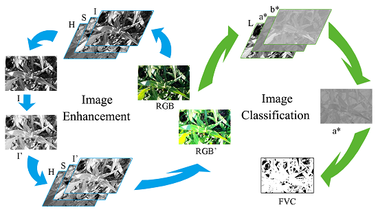
In this study, we propose a modified LABFVC algorithm that is shadow resistant and can classify green vegetation with reasonable accuracy. The whole method is realized in Matrix Laboratory (MATLAB; the MathWorks, USA) and can extract FVC automatically and efficiently. The accuracy of our method was evaluated using real and synthesized images.

2. Study Area and Data Processing

2.1. Study Area and Field Measurements

All data used in this article were obtained from the Heihe Watershed Allied Telemetry Experimental Research (HiWATER) field campaign conducted in the Heihe River basin, China [27]. Field measurements of FVC were taken in corn fields, orchards and fields planted with vegetables, such as peppers and red beans, from 24 May 2012 to 14 September 2012, every five days on average [28,29].
The land surface is relatively homogeneous in this area, and a patch of field was usually larger than 15 m × 15 m. This size matches the spatial scales of moderate-resolution satellites, e.g., the Advanced Spaceborne Thermal Emission and Reflection Radiometer (ASTER) [30]. A plot of 10 m × 10 m representing the scale of ASTER pixels was designed at every sampling position. Digital photographs were taken along two diagonals of the plot (taken once for the overlapping section at the cross point of the two diagonals). Twenty-two sampling plots were distributed throughout the area, of which 15 were located in corn fields. Nine photographs of each plot were taken. Approximately 4100 images were obtained during HiWATER 2012. Figure 1 shows the pattern in which photographs were taken in each plot.
Figure 1. Schematic of a plot showing how the photographs were taken. The nine small squares in the middle of the figure represent the photography positions in a plot. The large square around these squares represents the area of the sample plot.
Remotesensing 07 10425 g001

2.2. Data Description

2.2.1. Synthesized Images

The synthesized image was composed of different mosaics of digital images obtained in the HiWATER experiment, 2012 [29]. The reference FVC of the synthesized image can be exactly calculated as the ratio of the number of pixels of all vegetation mosaics to the total number of pixels in this image. Each of the square vegetation mosaics had 224 × 132 pixels. The entire synthesized image, with both vegetation and soil, had 2629 × 1765 pixels. The mosaics were derived from various images of leaves and soil, including those with deep shadows. Four different types of vegetation mosaics, namely bright-green vegetation, jade-green vegetation, bottle-green vegetation and shaded vegetation, were used to compose the vegetation part in the image (Table 1). Another four types of soil mosaics, namely, light-brown soil, brown soil, dark-grey soil and shaded soil, were selected to form the square image. The vegetation mosaics were regularly embedded in the synthesized image.
The shadow-resistant LABFVC (SHAR-LABFVC) algorithm proposed in this study, the LABFVC algorithm and visual interpretation were then implemented to process this image to evaluate the accuracy of these methods.
Table 1. Different mosaics composing the simulated picture.
VegetationRepresentationSoilRepresentation
Remotesensing 07 10425 i001Bright-green vegetation Remotesensing 07 10425 i002Light-brown soil
Remotesensing 07 10425 i003Jade-green vegetation Remotesensing 07 10425 i004Brown soil
Remotesensing 07 10425 i005Bottle-green vegetation Remotesensing 07 10425 i006Dark-grey soil
Remotesensing 07 10425 i007Shaded vegetation Remotesensing 07 10425 i008Shaded soil

2.2.2. Real Images

Fifteen real images of different crop types, including corn, peppers, cabbage, celery and beans, in different growing periods in 2012 were selected from HiWATER for comparison. All images were classified by visual interpretation, the LABFVC algorithm and SHAR-LABFVC. Visual interpretation was performed using Environment for Visualizing Images (ENVI; Exelis, Inc., Boulder, CO, USA) to obtain a reference FVC of the real images. First, we attempted to choose as many samples as possible and performed a supervised classification method using the maximum likelihood classifier. The image was divided into sunlit vegetation, shaded vegetation, sunlit soil and shaded soil. Then, the four classes were combined into two classes, namely vegetation and background, and an interactive tool was used to examine and correct the region of each class in the image. Finally, the proportion of vegetation was computed as the reference FVC of the image.

3. Methodology

SHAR-LABFVC was developed from and improves upon the work of Liu et al. [22], which is hereafter referred to as LABFVC. In the proposed algorithm, the hue saturation intensity (HSI) color space is introduced to decrease the difference between sunlit and shaded leaves. Subsequently, the image is transformed into the LAB color space, where the green red (a*) component is used to distinguish vegetation and background; negative a* values theoretically indicate green, and positive a* values indicate red. The distributions of green vegetation and background are respectively modeled with lognormal and Gaussian distribution functions on the a* component. The threshold is then calculated to classify the vegetation and background.

3.1. LABFVC Algorithm

The LABFVC algorithm proposed by Liu et al. [22] is an automatic FVC-extracting algorithm for digital images with an accuracy similar to that of the greenness (2G-R-B) method [31]. LABFVC is based on the premise that the representations of vegetation and soil in the LAB color spaces approximately follow Gaussian distributions. Therefore, green vegetation is classified by solving a Gaussian mixture model in the LAB color space. The threshold separating the vegetation from the background is automatically selected and used to calculate the FVC in an image.
The LABFVC algorithm consists of the following three steps:
First, the red-green-blue (RGB) digital image is converted to the LAB color space. The LAB color space is close to the human perception of color, and its channels are less correlated than those of the RGB color space [32]. Methods for transforming between RGB and LAB can be found in the references. The a* channel in the LAB color space is recommended for detecting green vegetation.
Second, assuming that the distributions of the vegetation and background in the a* dimension are Gaussian distributions, the following function can be used to fit the distribution of their frequency on the a* component:
F ( x ) = w v 2 π σ v e ( x μ v ) 2 2 σ v 2 + w b 2 π σ b e ( x μ b ) 2 2 σ b 2
where the dependent variable F is the frequency of the green vegetation and the background on the a* component; the independent variable x represents their a* values; μv and μb are the average values of the green vegetation and background, respectively; σv and σb are the standard deviations of the green vegetation and background, respectively; and wv and wb are the weights of the green vegetation and background, respectively.
Third, the threshold value T is determined based on the assumption that the probabilities of misclassifying vegetation and background are equal, which is used to classify the vegetation and background. After fitting the distributions of the vegetation and background by Equation (1), the average values of the green vegetation (μv) and background (μb), their standard deviations (σv and σb) and their weights (wv and wb) are known. Threshold T can be obtained by solving Equation (2):
w v e r f c ( T μ v 2 σ v ) = w b e r f c ( T μ b 2 σ b )
where the complementary error function erfc is incorporated to determine the threshold:
e r f c ( x ) = 1 e r f ( x ) = 2 π x e t 2 d t
where erf is the Gaussian error function.
The fraction of vegetation cover in an image is calculated after the vegetation is classified using the threshold T. For a more detailed description of the LABFVC algorithm, we refer to Liu et al. [22].

3.2. Shadow-Resistant LABFVC

Step 3 in the LABFVC method is identical to a step in SHAR-LABFVC, but Steps 1 and 2 are combined with new ideas to resist the shadow effect. In Figure 2, the following additional and improved processes are highlighted in yellow in the SHAR-LABFVC flow chart: (1) the use of the HSI color space to equalize the intensity histogram; and (2) fitting of the vegetation on the a* component of the LAB color space with a lognormal model.
Figure 2. Schematic of shadow-resistant SHAR-LABFVC (LAB, the Commission Internationale d’Eclairage L*a*b* color space; FVC, fractional vegetation cover). The portions highlighted in yellow are the main differences between the LABFVC algorithm and SHAR-LABFVC. a* is the green red component in the LAB color space. When a pixel’s a* value is smaller than the threshold T, the pixel is classified as green vegetation.
Remotesensing 07 10425 g002
In the first step of SHAR-LABFVC, the equalization of the intensity histogram aims to brighten the shaded leaves and to promote their separation probability. The HSI color space is chosen to enhance the intensity of the three components of an image in this color space, which are less correlated with each other than in the RGB color space [26]. For an RGB image, the intensity I of each pixel in HSI space is given by the following [26]:
I = 1 3 ( R + G + B )
To brighten the shaded leaves, we transform the RGB color space into the HSI space, select its intensity component, equalize the intensity histogram, replace the original intensity with the equalized one and retransform the image to the RGB color space.
In the second step (Figure 2), the distributions of the green vegetation and background are modeled on the a* component in the LAB color space, as in the LABFVC method. The modification to this step is that SHAR-LABFVC uses a lognormal model for the vegetation histogram. Green vegetation has a wide distribution on the negative axis of the a* component. The shaded vegetation is nearly black and has an a* value of approximately 0. Therefore, the complete color distribution of the vegetation is similar to a lognormal distribution. Figure 3 shows a histogram distribution of the a* component of an image of a corn field. The distribution of the background is assumed to be Gaussian, as in the LABFVC method.
Figure 3. Histogram of the a* (green red) component of an image. The green and brown curves represent the lognormal distribution of the vegetation and the Gaussian distribution of the background, respectively. The small image in the left corner is the original image.
Remotesensing 07 10425 g003
The following function can be used to fit the distributions of both the green vegetation and the background’s frequency on the a* component:
F ( x ) = w v x 2 π σ v e ( ln x μ v ) 2 2 σ v 2 + w b 2 π σ b e ( x μ b ) 2 2 σ b 2
where vegetation is fitted by a lognormal function.
In the third step, the green FVC is extracted by classifying the a* values of the images at the threshold T, determined using Equation (2). This step assumes that the misclassification probabilities of the vegetation and background are approximately equal. In Figure 4, sv and sb represent the areas of the misclassified vegetation and background, respectively. T is chosen such that sv and sb are equal.
Figure 4. Determining the threshold for image classification. The red curve is based on a lognormal distribution and represents the vegetation, and the black curve is based on a Gaussian distribution and represents the background. The classification is based on the a* (green red) component of the LAB color space.
Remotesensing 07 10425 g004

4. Results

4.1. Image Enhancement

Image enhancement is an important module in SHAR-LABFVC. Figure 5 shows the original, intensity-stretched and RGB stretched images, which present the effect of our image enhancement module. After the intensity histogram is equalized in the HSI color space, the entire image becomes brighter, particularly the shaded leaves in the red boxes (Figure 5b), facilitating the identification of shaded components. Equalizing all three components in the RGB color space can also highlight the shaded leaves, but changes the color of the image (Figure 5c). Therefore, stretching all of the RGB components is not usable when further classification of the vegetation is required.
Figure 5a was classified by visual interpretation, and the average values of the classes at the axis of the a* component are presented in Table 2, which also shows that the average values of the vegetation in the original image and the intensity-stretched image are both on the negative axis of the a* component. As shown in Table 2, the difference between the vegetation and background in the intensity-stretched image is greater than that in the original image. Image enhancement effectively enhances the difference between the vegetation and background and can help separate these two classes.
Figure 5. Image enhancement in different color spaces and the classification result. (a) The original image. (b) The intensity-stretched image after transformation to the HSI color space and intensity histogram equalization. (c) The RGB stretched image, in which the histograms of the three components (R, G, B) have been equalized separately. (d) The SHAR-LABFVC classification result. The red boxes marked with the same number in images (a), (b), (c) and (d) represent the same area.
Remotesensing 07 10425 g005
Table 2. Average values of the different classes and their differences in the image’s a* component with different image enhancement methods.
DataVegetationBackgroundDistance*
The original picture−17.2040.70817.912
Intensity-stretched picture−30.5391.41831.957
RGB stretched picture−0.57615.29915.875
* The distance represents the difference between the averaged values of two parts.

4.2. Analysis and Evaluation of the Synthesized Image

The synthesized image was used to compare SHAR-LABFVC, LABFVC and visual interpretation. The classification results are presented in Figure 6. Table 3 presents the FVC estimates. The result for SHAR-LABFVC is 0.237, identical to the reference FVC (0.237). The result for the LABFVC algorithm is lower, because it cannot distinguish leaves with deep shadows from the background (Figure 6c).
Figure 6. (a) The synthesized image and classification using (b) visual interpretation, (c) LABFVC and (d) SHAR-LABFVC. The white and black regions were classified as vegetation and soil, respectively.
Remotesensing 07 10425 g006
Table 3. Reference FVC and FVC estimates from the synthesized image test.
ApproachFVC
The Reference FVC *0.237
LABFVC0.209
SHAR-LABFVC0.237
* The reference FVC is equal to the proportion of the area of all vegetation mosaics in the synthesized image.

4.3. Analysis and Evaluation Based on Real Images

4.3.1. Different Types and Growth Stages of Vegetation

Fifteen real images from different crop types and different growing periods were selected for the evaluation. All images were classified strictly and carefully by visual interpretation via ENVI to obtain the reference FVC of the real images. Table 4 presents the classification accuracy of each image. In this evaluation, the average overall accuracy of visual interpretation was 99.54%.
Table 5 presents the comparison of the results of the methods for 15 randomly-selected real images that were carefully interpreted visually. When the vegetation is sparse, the reference FVC is less than 0.5, and the RMSEs of the two methods are similar. When the vegetation increases, the reference FVC is greater than 0.5, and the two methods appear different. Based on the reference FVC determined by visual interpretation, the RMSE of SHAR-LABFVC is 0.025. However, the RMSE of LABFVC is as high as 0.1. As the density of the vegetation increases, shadows deepen and influence the performance of LABFVC.
Table 4. Accuracy evaluation of the visual interpretation of the 15 real images.
ImageCrop TypeProduct Accuracy (%)User Accuracy (%)Overall Accuracy (%)Kappa Coefficient
VegetationBackgroundVegetationBackground
1corn94.10100.00100.0088.6095.960.9093
2corn99.9499.9499.9999.7799.940.9982
3corn98.68100.00100.0099.6099.700.9914
4corn100.00100.00100.00100.00100.001.0000
5corn100.0099.3499.91100.0099.920.9962
6bell pepper100.00100.00100.00100.00100.001.0000
7bell pepper99.4299.88100.0099.8199.760.9936
8hot pepper96.83100.00100.0098.5999.020.9768
9hot pepper100.0099.81100.00100.0099.930.9985
10celery99.9199.4899.6099.8899.720.9943
11celery99.9599.9199.9699.9899.940.9986
12cabbage99.99100.00100.0099.99100.000.9999
13cabbage100.00100.00100.0099.99100.000.9999
14sapling98.79100.00100.0098.8499.400.9880
15sapling99.9799.5799.6499.9899.790.9957
Table 5. Evaluation of the LABFVC algorithm and SHAR-LABFVC.
ApproachRMSE
FVC < 0.5FVC > 0.5
LABFVC0.0220.100
SHAR-LABFVC0.0250.025
Example results of the comparison are displayed in Figure 7 and Figure 8. The two original images shown here were captured in July when the plants were in their lush vegetation period. Figure 8a was taken on a cloudy day; thus, the differences between the results of visual interpretation, SHAR-LABFVC and the LABFVC algorithm are small (Figure 8 and Table 6). Figure 7a was taken on a sunny day; thus, the difference between sunlit and shaded leaves tends to be large, and the advantages of SHAR-LABFVC become important (Figure 7 and Table 6).
Table 6. FVC estimates of the real images.
ApproachFigure 7Figure 8
Visual interpretation0.9090.791
LABFVC0.6670.738
SHAR0.9020.799
Figure 7. A digital image and its classification results. (a) The original image of corn. (b) An enlarged view of the red box in (a). The classification results of (c) visual interpretation, (d) the LABFVC algorithm and (e) SHAR-LABFVC. In (c–e), the black and white areas are classified as background and vegetation, respectively. The red boxes in pictures represent the same area.
Remotesensing 07 10425 g007
Figure 8. The same as Figure 7, except that the original image is of celery. (a) The original image of celery. (b) An enlarged view of the red box in (a). The classification results of (c) visual interpretation, (d) the LABFVC algorithm and (e) SHAR-LABFVC. In (c–e), the black and white areas are classified as background and vegetation, respectively. The red boxes in pictures represent the same area.
Remotesensing 07 10425 g008

4.3.2. Extreme Situations

Four extreme situations, including no shadow (Figure 9A), many shallow shadows (Figure 9B), no leaf (Figure 9C) and many leaves with deep shadows (Figure 9D), are represented in the corn images taken under different illumination conditions and growth periods. These images were carefully classified using visual interpretation via ENVI to obtain the reference FVC. The classification results are shown in Figure 9 and Table 7.
Figure 9. The classification results in four extreme situations. (A1) was taken on a cloudy day, when there was no shadow. (B1) was taken on a sunny day, when there were many shallow shadows covering both the vegetation and background. (C1) was taken in the Gobi desert, where there is seldom green vegetation. (D1) was taken when the corn was fully grown and there were limited gaps between the leaves. The images in Columns (24) are the classification results from visual interpretation, LABFVC and SHAR-LABFVC, respectively.
Remotesensing 07 10425 g009
Table 7. FVC estimates of each extreme situation.
ImageSituationApproach
Visual InterpretationLABFVCSHAR-LABFVC
ANo shadow0.5790.5590.563
BFull of shallow shadows0.6830.6740.684
CNo leaf0.0000.0000.003
DFull of leaves 0.9420.6420.922

4.4. Comparison with Time Series Data

The results of the LABFVC algorithm and SHAR-LABFVC were compared for the 15 corn plots of the 2012 HiWATER experiment. The results of the comparison are shown in Figure 10. The two results were quite similar before 26 June, when the corn was young and the leaves did not shade each other significantly. As the crop matured, the underestimation of LABFVC became obvious. For example, on 13 July, the LABFVC algorithm underestimated the result by more than 0.2. After August, when corn was harvested and the leaves had turned yellow, the FVC determined by the different methods exhibited fewer differences.
Figure 10. Comparison of the results of the LABFVC algorithm and SHAR-LABFVC over the entire growing period of corn. Error bars represent the positive and negative standard errors of the mean.
Remotesensing 07 10425 g010

5. Discussion

Shadows occur due to obstructions from terrain topography, cloud cover or dense vegetation and can cause errors in image classification. In this study, we proposed an automatic shadow-resistant FVC extraction method (SHAR-LABFVC) that can classify green vegetation efficiently and achieve stable results with reasonable accuracy.
SHAR-LABFVC was developed based on LABFVC, which was chosen because of its automaticity and efficiency [26]. SHAR-LABFVC can automatically determine the threshold to classify green vegetation and to compute FVC from digital images. In contrast to the supervised classification [13,14] and other image analysis approaches based on physical characteristics [15,16], neither LABFVC nor SHAR-LABFVC require manual steps to process images.
The time required to extract FVC using LABFVC is less than 12 seconds per image, much faster than other automated image classification methods based on physical characteristics (PC-based) [16] and approaches for feature space analysis (FSA-based) [12] (Table 8). The time required to extract FVC using SHAR-LABFVC is approximately five seconds per image. SHAR-LABFVC is thus sufficiently efficient for real-time application.
Table 8. Average computing time of the different methods.
ApproachTime (per image)Computer ProcessorRandom-AccessMemory (RAM)Program/Software
PC-based *15 min--eCognition 8.7 (Trimble Navigation Ltd. USA)
FSA-based *91.9 s1.2 GHz512 MBVC++
LABFVC12.0 s3.1 GHz4 GBMATLAB
SHAR-LABFVC5.0 s3.1 GHz4 GBMATLAB
* The efficiency for the PC-based and the FSA-based methods was determined based on the work of Bauer et al. [16] and Zheng et al. [12].
Real and synthesized image evaluation results were presented in Section 4.2 and Section 4.3. The classification accuracy of the real images (Table 4) and the process of image synthesis (Section 2.2.1) indicate a high reliability of the reference values.
The LABFVC algorithm works well when the vegetation is sparse. However, LABFVC is more sensitive to the contrast between sunlit parts and shadows, which causes systematic errors in classification. With the use of image enhancement and lognormal distribution, SHAR-LABFVC is much less sensitive to the shadow effect than LABFVC. Image enhancement was introduced to decrease the shadow effect, which is more convenient to implement than using artificial shelters to change the illumination conditions [21,25]. In contrast to other image analysis approaches [15,16], SHAR-LABFVC brightens and separates the shaded vegetation and background rather than classifying shadow as another class. This process also improves the accuracy of obtained green FVC.
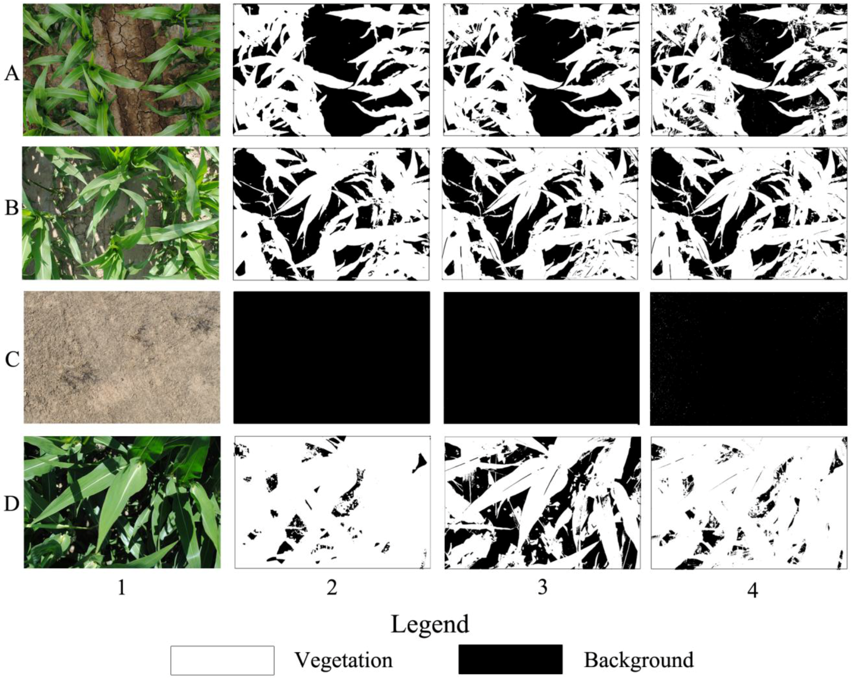
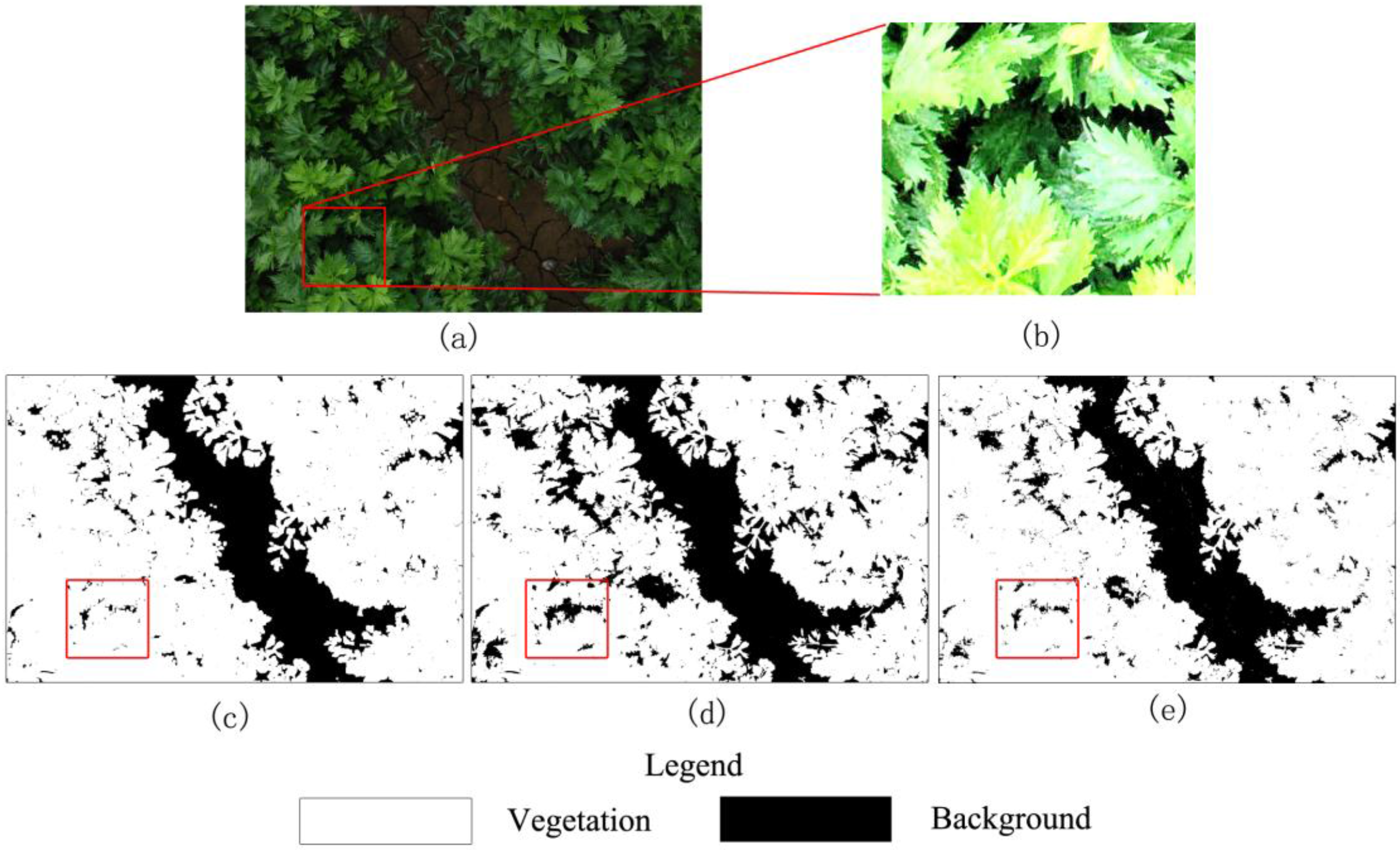
SHAR-LABFVC was designed to extract FVC from the images taken with a digital camera. Photography is a commonly-used method for obtaining FVC from crop, grassland, low shrub areas and understory in sparse forests. When the digital image contains heavily-shaded parts, LABFVC cannot obtain vegetation efficiently. Compared to LABFVC, SHAR-LABFVC obtains results more similar to the reference FVC, particularly when heavily-shaded components are present. Representing the extreme situations that may appear in these areas, the classification results for images with no shadow, many shadows, no leaves and many leaves with deep shadows are shown in Figure 9. When no shadow or a few shadows cover the vegetation or background (Figure 9A1, B1 and C1), the differences among the results of LABFVC, SHAR-LABFVC and visual interpretation are small. When the leaves heavily shade one another (Figure 9D1), shadows tend to be dark and LABFVC significantly underestimates the vegetation (Figure 9D3).
Time series images of corn were processed to evaluate the accuracy of SHAR-LABFVC (Figure 10). The results of SHAR-LABFVC and LABFVC are quite similar during both the budding period and the period when leaves are withered. When the crops mature, leaves significantly shade the incoming light from the Sun and the sky. Deep shadows occur during this period, and the advantages of SHAR-LABFVC are apparent.
SHAR-LABFVC is shadow-resistant and reliable based on the evaluations. However, there are still some shortfalls in SHAR-LABFVC. 
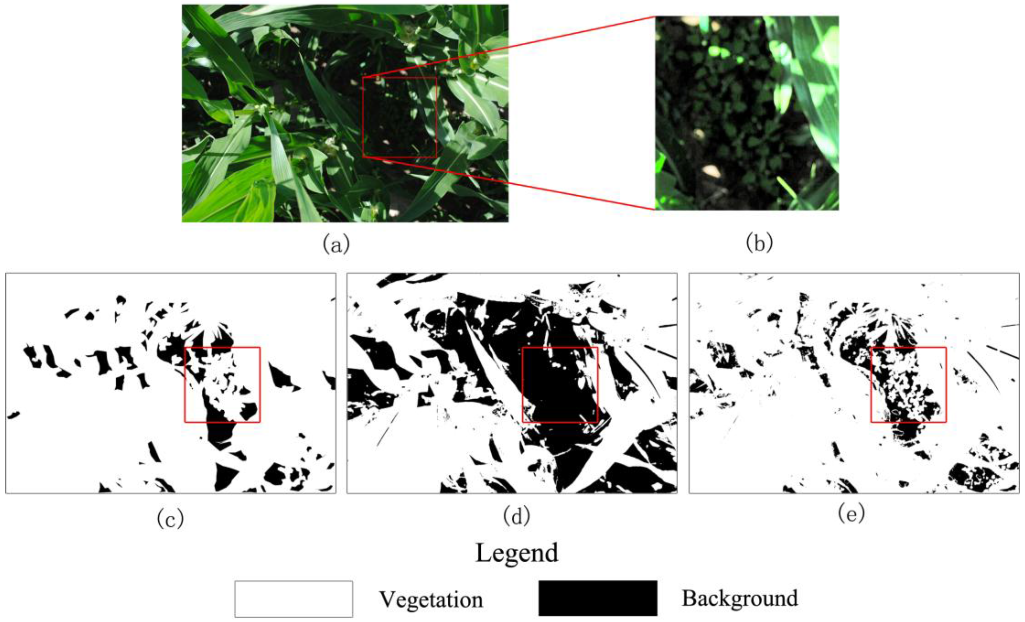
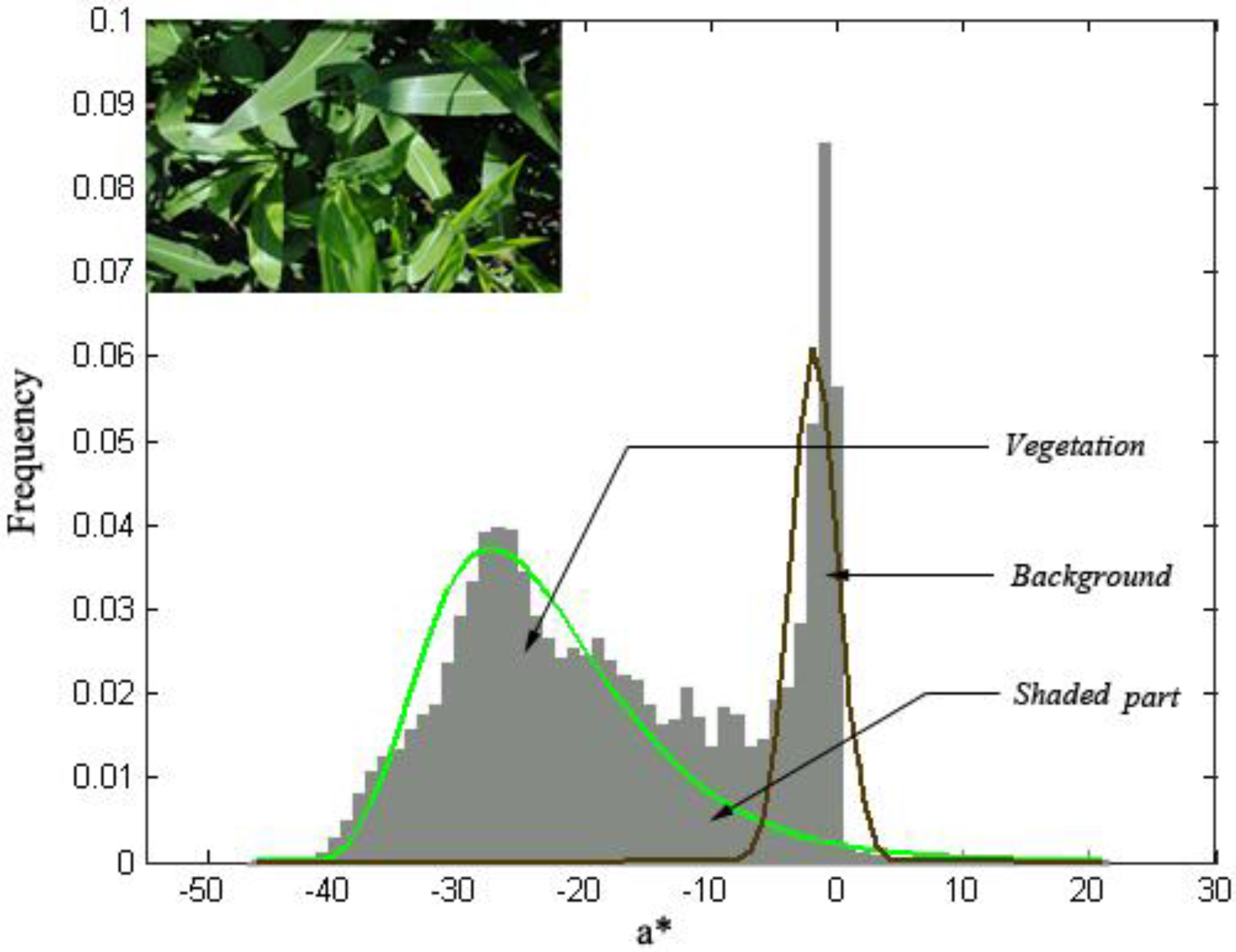
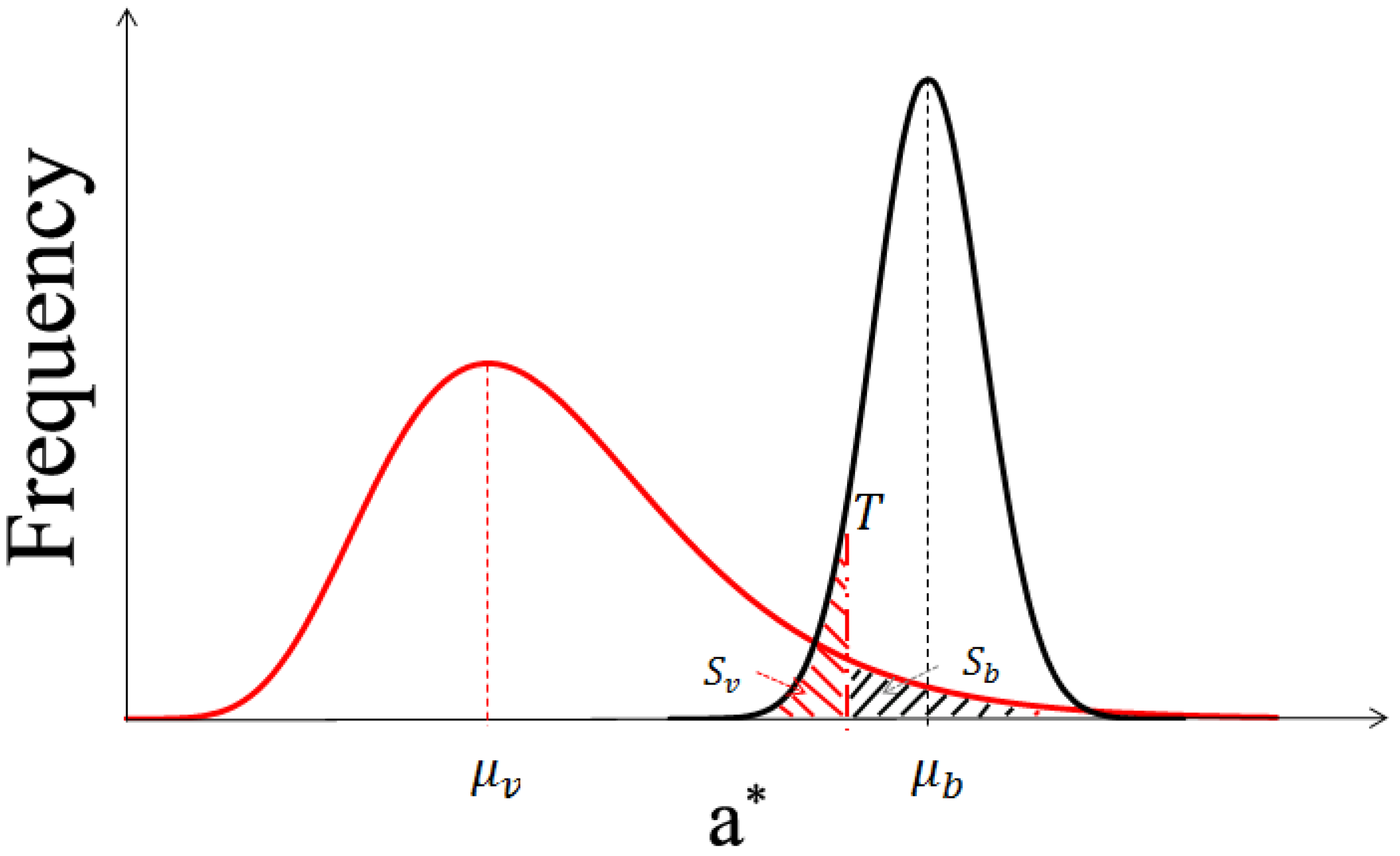
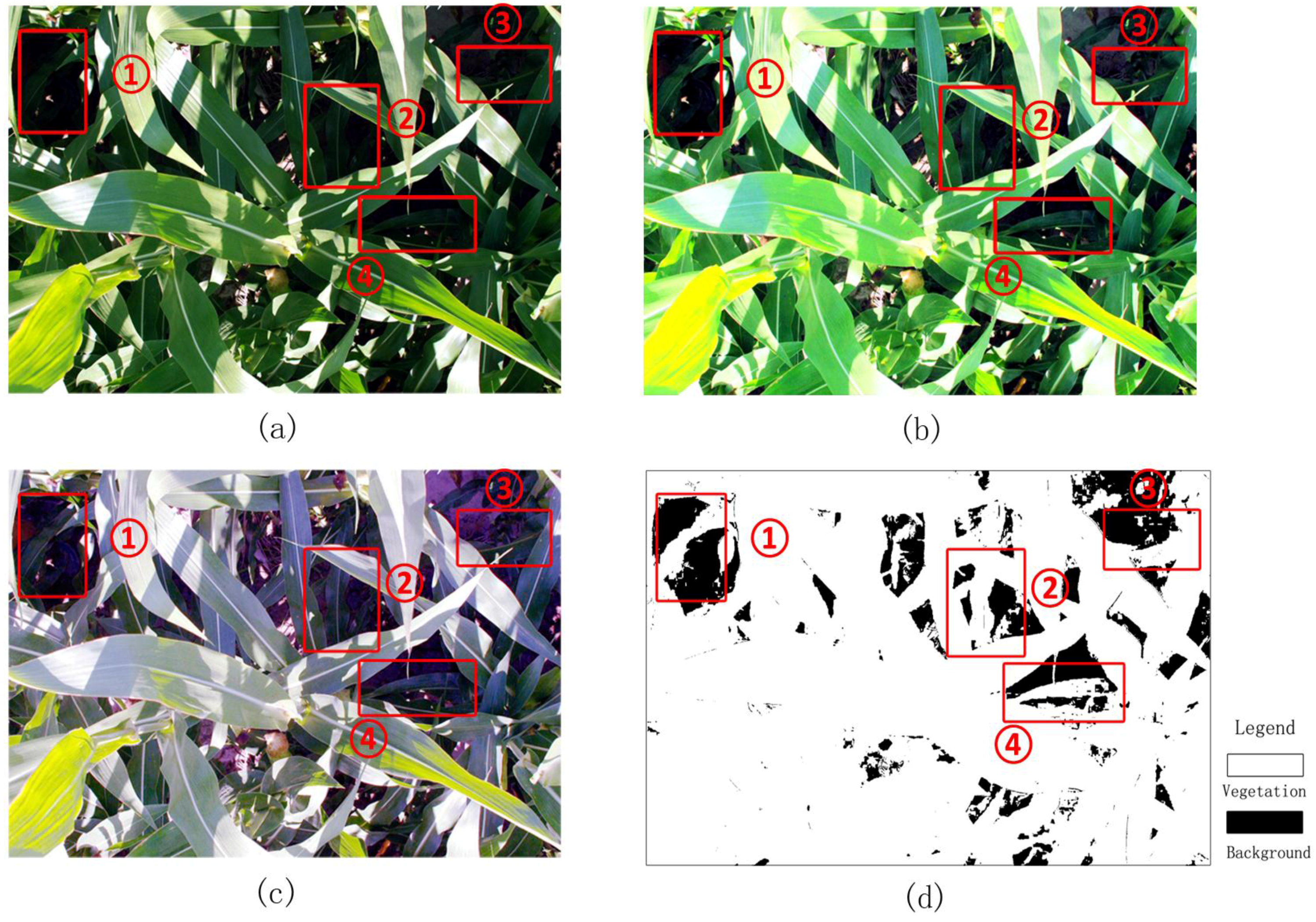
Figure 7 presents a case in which the corn plants are tall and project many deep shadows that cover more than half of the image. Figure 7c shows that visual interpretation produces a smooth classification image. The main differences between the classification methods can be observed in the area in which the leaves are crimped or overlap with one another and generate dark shadows. Some shaded leaves are too dark to be stretched by SHAR-LABFVC. The leaf veins and solar glints also cause classification errors because they are extremely bright and nearly white. After adjusting the intensity, these leaves are still saturated and far from green. These situations correspond to the parts of the soil and vegetation histograms that are mixed in the image’s a* component (areas sv and sb in Figure 3), resulting in misclassification. Generally, the FVC estimates provided by SHAR-LABFVC are fairly close to those of visual interpretation under all possible illumination conditions.

6. Conclusions

Deep shadows severely affect the results of digital image classification, particularly when vegetation growth is at its peak. In this study, we developed a shadow-resistant LABFVC algorithm (SHAR-LABFVC) to extract FVC from digital images. SHAR-LABFVC improves the documented LABFVC method and resists shadows by equalizing the histogram of the image’s intensity component in the HSI color space and brightening the shaded parts of the leaves and background. Generally, the histogram of the vegetation’s green red component exhibits a lognormal distribution because of the shaded leaves. This property is considered when dividing the images into vegetation and background regions in the LAB (the Commission Internationale d’Eclairage L*a*b*) color space.
The evaluation of SHAR-LABFVC revealed high accuracy similar to that of visual interpretation. The latter is assumed to be an accurate classification method that allows a reference FVC to be obtained from a digital image. As demonstrated by the results of this study, the RMSE of SHAR-LABFVC based on visual interpretation is 0.025, indicating similar performances of SHAR-LABFVC and visual interpretation. However, SHAR-LABFVC is more pragmatic and automatic. Compared to other automatic classification methods based on physical characteristics or feature space analysis, SHAR-LABFVC is less time consuming. Thus, SHAR-LABFVC can be used to obtain the FVCs of a large number of images.
Shadows caused errors of up to 0.2 when estimating FVC at moderate resolutions (e.g., the scale of ASTER) in the flourishing vegetation period. This underestimation of FVC caused by shadow effects will also affect the evaluation of present global FVC products at coarse resolutions (e.g., 1 km), because the systematic errors of moderate-spatial resolution FVC cannot be eliminated in the up-scaling process. Therefore, the development of shadow-resistant algorithms for field measurements is required. Given the uncertainties in our algorithm, further research is needed to investigate additional vegetation types and data sources. However, SHAR-LABFVC is expected to facilitate the validation of satellite-based products in this context due to its efficiency.

Acknowledgments

This work was supported by the key program of National Natural Science Foundation of China (NSFC) (Grant No. 91125004), the NSFC (Grant No.41331171), the National Basic Research Program of China (973 Program) (Grant No. 2013CB733402) and the National High Technology Research and Development Program (863 Program) (Grant No. 2012AA12A305).

Author Contributions

Wanjuan Song improved LABFVC, proposed SHAR-LABFVC for FVC extraction and wrote the manuscript. Xihan Mu guided the entire research project, designed the structure of the manuscript and revised the manuscript. Guangjian Yan helped revise the manuscript. Shuai Huang prepared the digital images used in the manuscript.

Conflicts of Interest

The authors declare no conflict of interest.

References

  1. Gutman, G.; Ignatov, A. The derivation of the green vegetation fraction from NOAA/AVHRR data for use in numerical weather prediction models. Int. J. Remote Sens. 1998, 19, 1533–1543. [Google Scholar] [CrossRef]
  2. Hirano, Y.; Yasuoka, Y.; Ichinose, T. Urban climate simulation by incorporating satellite-derived vegetation cover distribution into a mesoscale meteorological model. Theor. Appl. Climatol. 2004, 79, 175–184. [Google Scholar] [CrossRef]
  3. Jiapaer, G.; Chen, X.; Bao, A. A comparison of methods for estimating fractional vegetation cover in arid regions. Agric. Forest Meteorol. 2011, 151, 1698–1710. [Google Scholar] [CrossRef]
  4. Zhao, C.; Li, Z.; Lv, H.; Li, T.; Hu, T.; Zhai, H.; Wang, H.; Li, Y.; Wang, Z.; Chang, Z.; et al. Vegetation Cover degree monitoring in Helanshan Mountain Project area of Sino-Germany Cooperation Ningxia Shelter-Forest Project. Ningxia J. Agric. For. Sci. Technol. 2000, S1, 6–14, (In Chinese with English Abstract). [Google Scholar]
  5. Zhou, Q.; Robson, M.; Pilesjo, P. On the ground estimation of vegetation cover in Australian rangelands. Int. J. Remote Sens. 1998, 19, 1815–1820. [Google Scholar] [CrossRef]
  6. Hu, Z.-Q.; He, F.-Q.; Yin, J.-Z.; Lu, X.; Tang, S.-L.; Wang, L.-L.; Li, X.-J. Estimation of fractional vegetation cover based on digital camera survey data and a remote sensing model. J. China Univ. Min. Technol. 2007, 17, 116–120. [Google Scholar] [CrossRef]
  7. Wimbush, D.J.; Barrow, M.D.; Costin, A.B. Color stereophotography for the measurement of vegetation. Ecology 1967, 48, 150–152. [Google Scholar] [CrossRef]
  8. Wells, K.F. Measuring vegetation changes on fixed quadrats by vertical ground stereophotography. J. Range Manag. Arch. 1971, 24, 233–236. [Google Scholar] [CrossRef]
  9. Purevdorj, T.S.; Tateishi, R.; Ishiyama, T.; Honda, Y. Relationships between percent vegetation cover and vegetation indices. Int. J. Remote Sens. 1998, 19, 3519–3535. [Google Scholar] [CrossRef]
  10. Alganci, U.; Ozdogan, M.; Sertel, E.; Ormeci, C. Estimating maize and cotton yield in southeastern Turkey with integrated use of satellite images, meteorological data and digital photographs. Field Crop. Res. 2014, 157, 8–19. [Google Scholar] [CrossRef]
  11. Kirci, M.; Gunes, E.O.; Cakir, Y.; Senturk, S. Vegetation measurement using image processing methods. In Proceedings of the IEEE Third International Conference on Agro-Geoinformatics, Beijing, China, 11–14 August 2014; pp. 1–5.
  12. Zheng, L.; Zhang, J.; Wang, Q. Mean-shift-based color segmentation of images containing green vegetation. Comput. Electron. Agric. 2009, 65, 93–98. [Google Scholar] [CrossRef]
  13. Fernández-Pacheco, D.G.; Escarabajal-Henarejos, D.; Ruiz-Canales, A.; Conesa, J.; Molina-Martínez, J.M. A digital image-processing-based method for determining the crop coefficient of lettuce crops in the southeast of Spain. Biosyst. Eng. 2014, 117, 23–34. [Google Scholar] [CrossRef]
  14. Escarabajal-Henarejos, D.; Molina-Martínez, J.M.; Fernández-Pacheco, D.G.; Cavas-Martínez, F.; García-Mateos, G. Digital photography applied to irrigation management of Little Gem lettuce. Agric. Water Manag. 2015, 151, 148–157. [Google Scholar] [CrossRef]
  15. Laliberte, A.S.; Rango, A.; Herrick, J.E.; Fredrickson, E.L.; Burkett, L. An object-based image analysis approach for determining fractional cover of senescent and green vegetation with digital plot photography. J. Arid Environ. 2007, 69, 1–14. [Google Scholar] [CrossRef]
  16. Bauer, T.; Strauss, P. A rule-based image analysis approach for calculating residues and vegetation cover under field conditions. Catena 2014, 113, 363–369. [Google Scholar] [CrossRef]
  17. Kataoka, T.; Kaneko, T.; Okamoto, H.; Hata, S. Crop growth estimation system using machine vision. In Proceedings of the IEEE/ASME International Conference on Advanced Intelligent Mechatronics, Kobe, Japan, 20–24 July 2003.
  18. Gée, C.; Bossu, J.; Jones, G.; Truchetet, F. Crop/weed discrimination in perspective agronomic images. Comput. Electron. Agric. 2008, 60, 49–59. [Google Scholar] [CrossRef]
  19. Woebbecke, D.M.; Meyer, G.E.; Von Bargen, K.; Mortensen, D.A. Color indices for weed identification under various soil, residue, and lighting conditions. Trans. ASAE 1995, 38, 259–269. [Google Scholar] [CrossRef]
  20. Neto, J.C.; Meyer, G.E.; Jones, D.D. Individual leaf extractions from young canopy images using Gustafson–Kessel clustering and a genetic algorithm. Comput. Electron. Agric. 2006, 51, 66–85. [Google Scholar] [CrossRef]
  21. Sakamoto, T.; Shibayama, M.; Kimura, A.; Takada, E. Assessment of digital camera-derived vegetation indices in quantitative monitoring of seasonal rice growth. ISPRS J. Photogramm. Remote Sens. 2011, 66, 872–882. [Google Scholar] [CrossRef]
  22. Liu, Y.; Mu, X.; Wang, H.; Yan, G. A novel method for extracting green fractional vegetation cover from digital images. J. Veg. Sci. 2012, 23, 406–418. [Google Scholar] [CrossRef]
  23. Macfarlane, C.; Ogden, G.N. Automated estimation of foliage cover in forest understorey from digital nadir images. Methods Ecol. Evol. 2012, 3, 405–415. [Google Scholar] [CrossRef]
  24. Sykes, J.M.; Horrill, A.D.; Mountford, M.D. Use of visual cover assessments as quantitative estimators of some British woodland taxa. J. Ecol. 1983, 71, 437–450. [Google Scholar] [CrossRef]
  25. Booth, D.T.; Cox, S.E.; Louhaichi, M.; Johnson, D.E. Technical note: Lightweight camera stand for close-to-earth remote sensing. Rangel. Ecol. Manage. 2004, 57, 675–678. [Google Scholar] [CrossRef]
  26. Gonzalez, R.C.; Woods, R.E. Digital Image Processing; Prentice Hall: Upper Saddle River, NJ, USA, 2009. [Google Scholar]
  27. Li, X.; Cheng, G.; Liu, S.; Xiao, Q.; Ma, M.; Jin, R.; Che, T.; Liu, Q.; Wang, W.; Qi, Y.; et al. Heihe watershed allied telemetry experimental research (HiWATER): Scientific objectives and experimental design. Bull. Am. Meteorol. Soc. 2013, 94, 1145–1160. [Google Scholar] [CrossRef]
  28. Mu, X.; Huang, S.; Ren, H.; Yan, G.; Song, W.; Ruan, G. Validating GEOV1 Fractional Vegetation Cover derived from coarse-resolution remote sensing images over croplands. IEEE J. Sel. Top. Appl. Earth Obs. Remote Sens. 2014, 8, 439–446. [Google Scholar] [CrossRef]
  29. Mu, X.; Huang, S.; Chen, Y. HiWATER:Dataset of Fractional Vegetation Cover in the middle Reaches of the Heihe River Basin; Beijing Normal University: Beijing, China; Cold and Arid Regions Environmental and Engineering Research Institute, Chinese Academy of Sciences: Lanzhou, China, 2013; (In Chinese). [Google Scholar] [CrossRef]
  30. Goward, S.N.; Arvidson, T.; Williams, D.L.; Irish, R.; Irons, J. Moderate spatial resolution optical sensors. In The SAGE Handbook of Remote Sensing; Warner, T.A., Nellis, M.D., Foody, G.M., Eds.; SAGE Publications Ltd: London, UK, 2009; pp. 123–139. [Google Scholar]
  31. Liu, J.; Pattey, E. Retrieval of leaf area index from top-of-canopy digital photography over agricultural crops. Agric. For. Meteorol. 2010, 150, 1485–1490. [Google Scholar] [CrossRef]
  32. Yam, K.L.; Papadakis, S.E. A simple digital imaging method for measuring and analyzing color of food surfaces. J. Food Eng. 2004, 61, 137–142. [Google Scholar] [CrossRef]

