
The Sentinel-1 Mission: New Opportunities for Ice Sheet Observations


Abstract
:
1. Introduction
2. Data Sources


| Satellite | SAR Frequency (GHz) | Repeat Cycle (Day) | Imaging Mode | Swath (km) | Incidence Angle (deg) | Nominal Resolution Gr × Az (m) | Pixel Spacing LOS Az (m) |
|---|---|---|---|---|---|---|---|
| Sentinel-1 | 5.4 | 12 | IW | 250 | 30–42 | 5 20 | 2.4 13.9 |
| TerraSAR-X | 9.6 | 11 | SM | 30 | 28–42 * | 2 3.3 | 0.9 1.95 |
| ALOS | 1.27 | 46 | FBS | 70 | 34 | 7 5 | 4.7 3.6 |
3. Methods
| Sentinel-1 IW | TerraSAR-X | ALOS PALSAR | |
|---|---|---|---|
| Matching window size Pixels (LOS azimuth) | 144 48 | 72 72 | 144 144 |
| Sampling steps Pixels (LOS azimuth) | 40 20 | 20 20 | 32 32 |
| Velocity product, Grid spacing in meters (Easting Northing) | 250 250 * 30 × 30 # | 30 30 | 30 30 |
4. Results
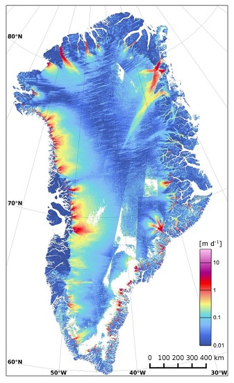
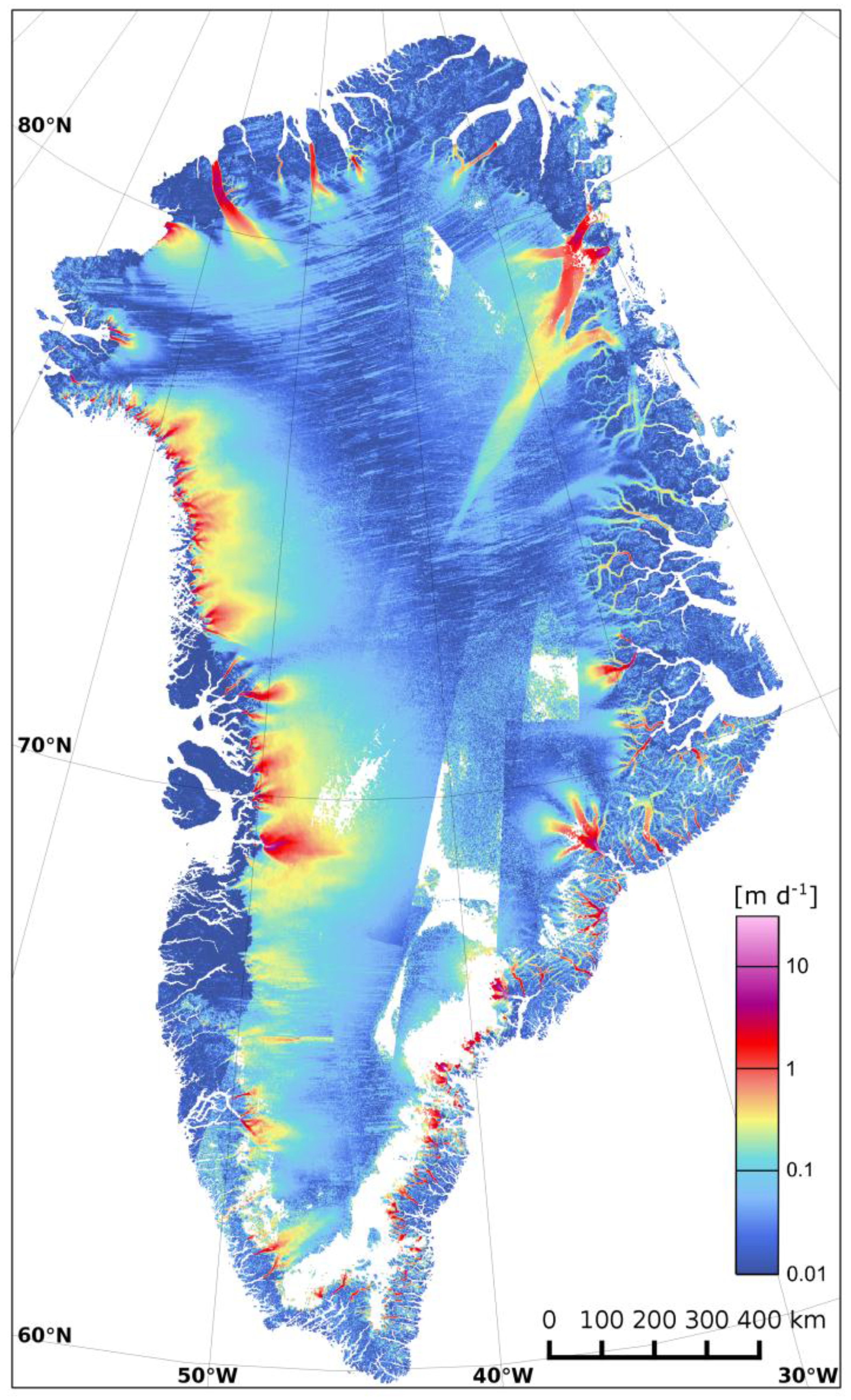
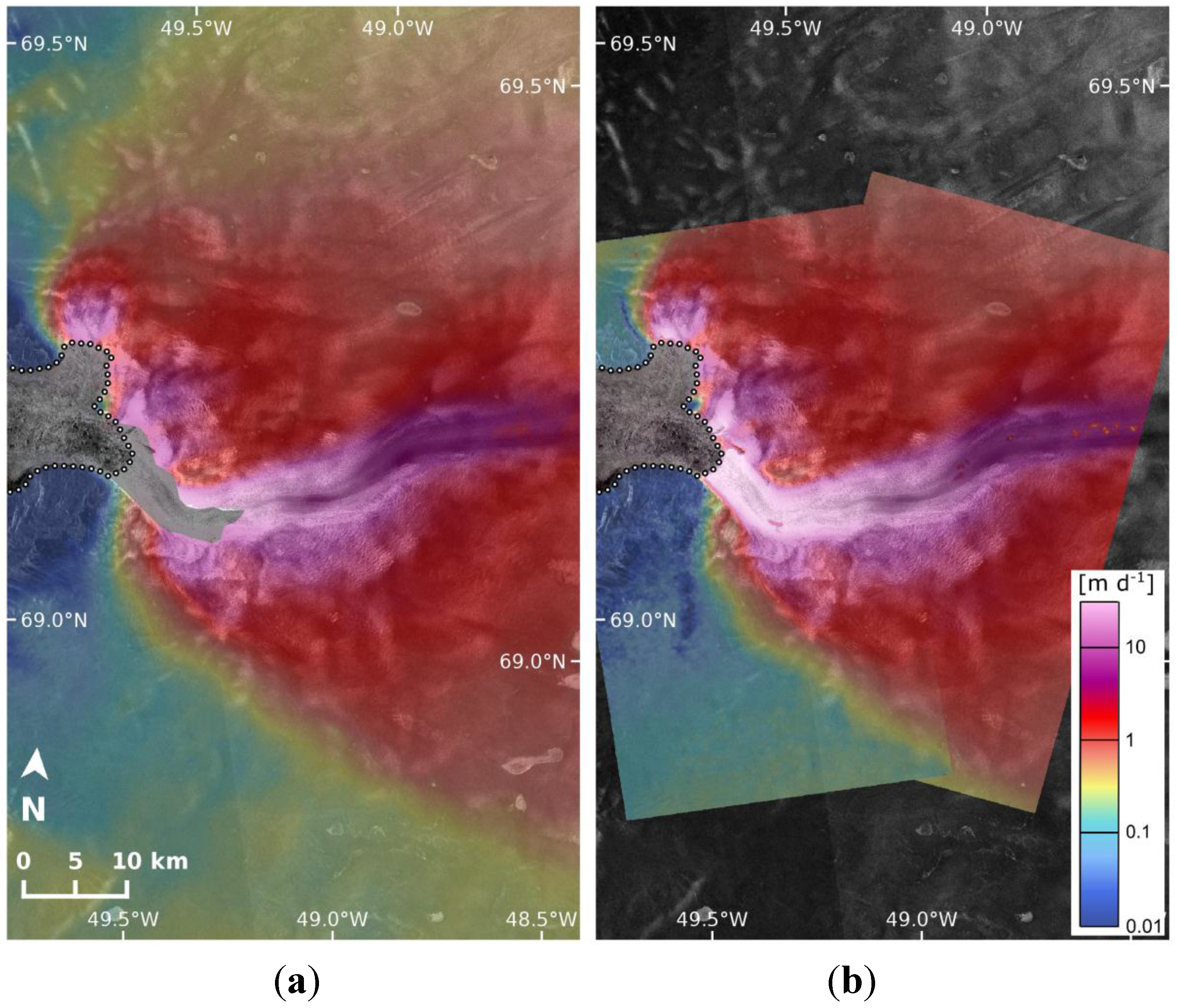
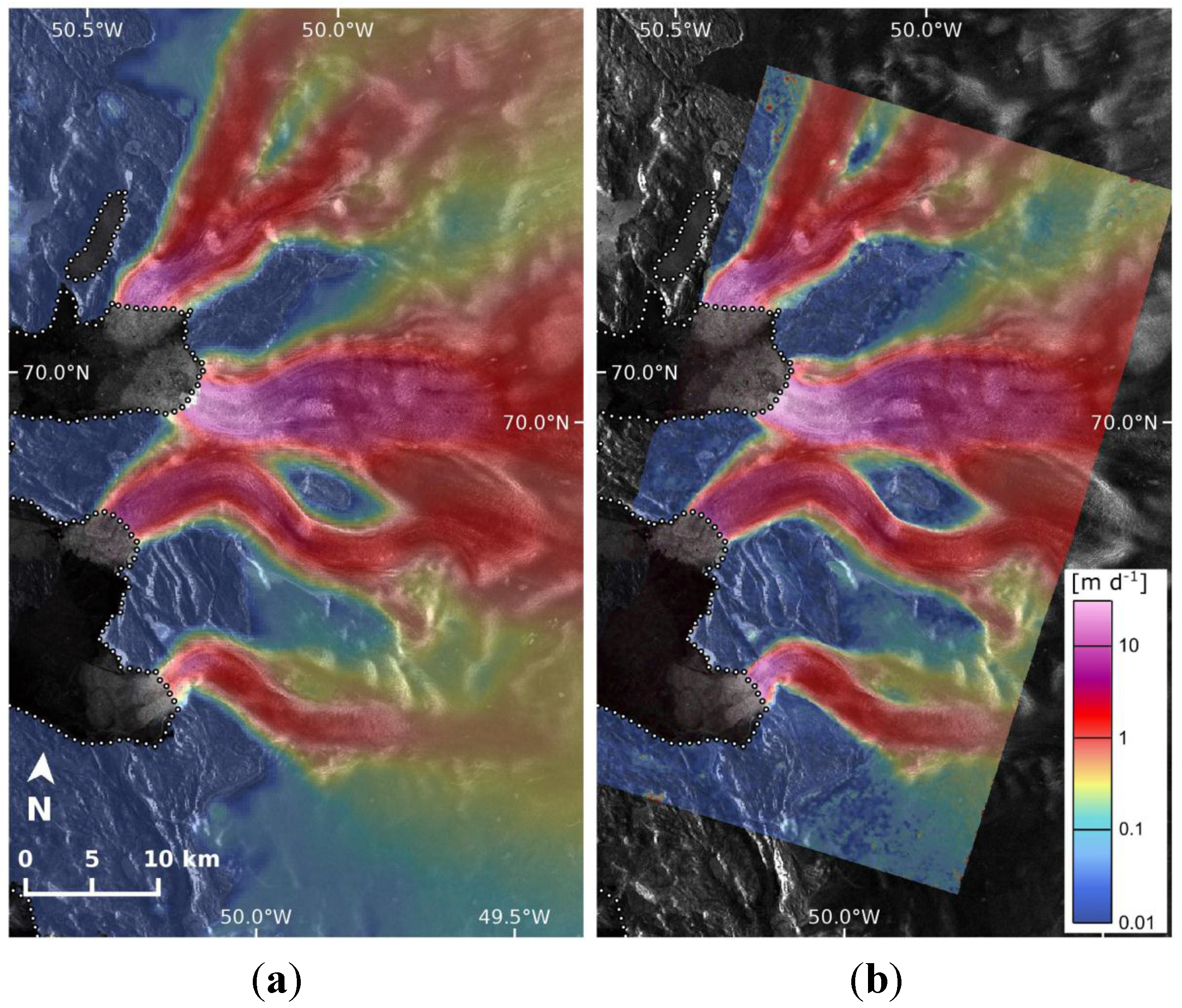
4.1. Sentinel-1 Ice Velocity Map
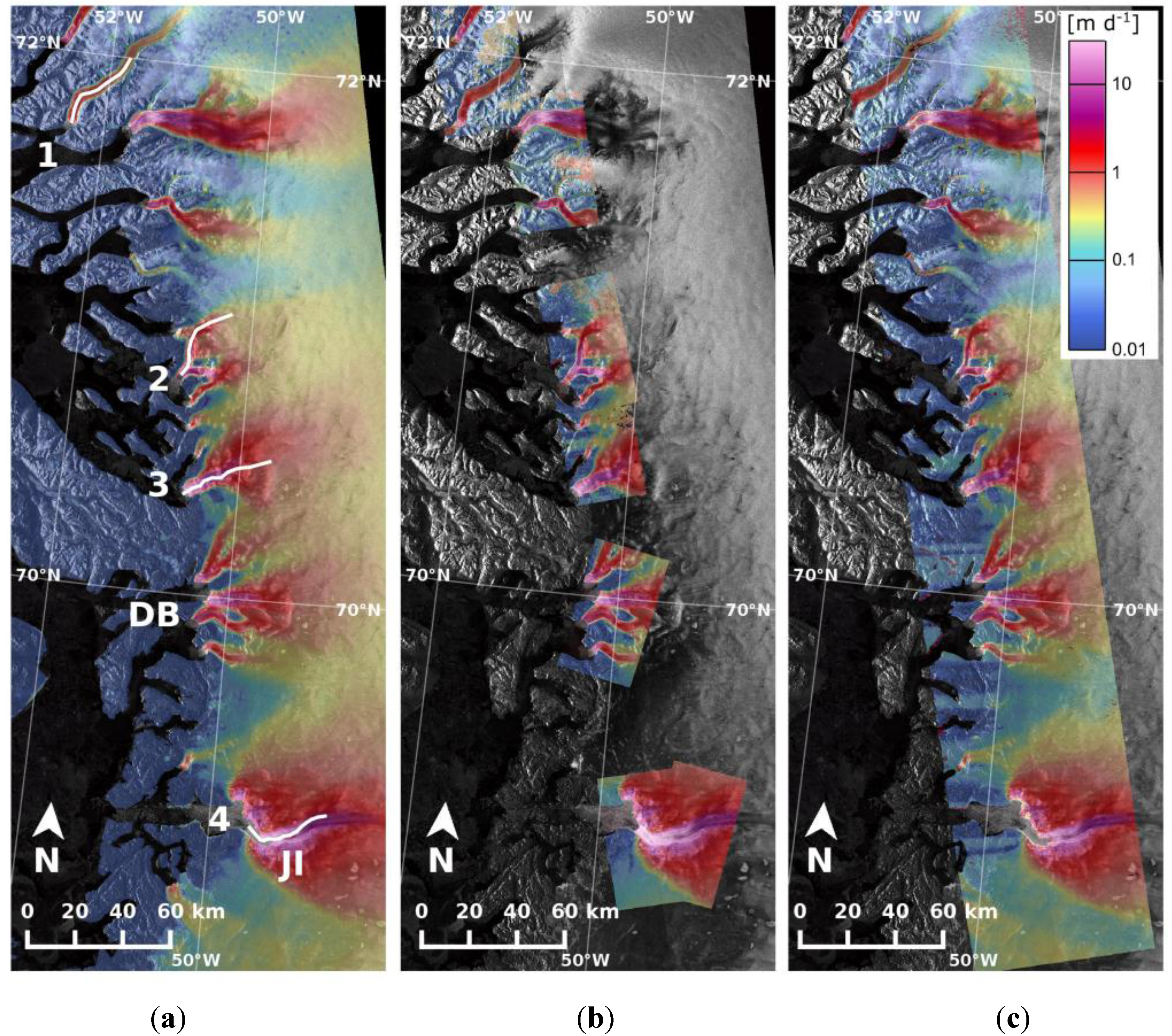
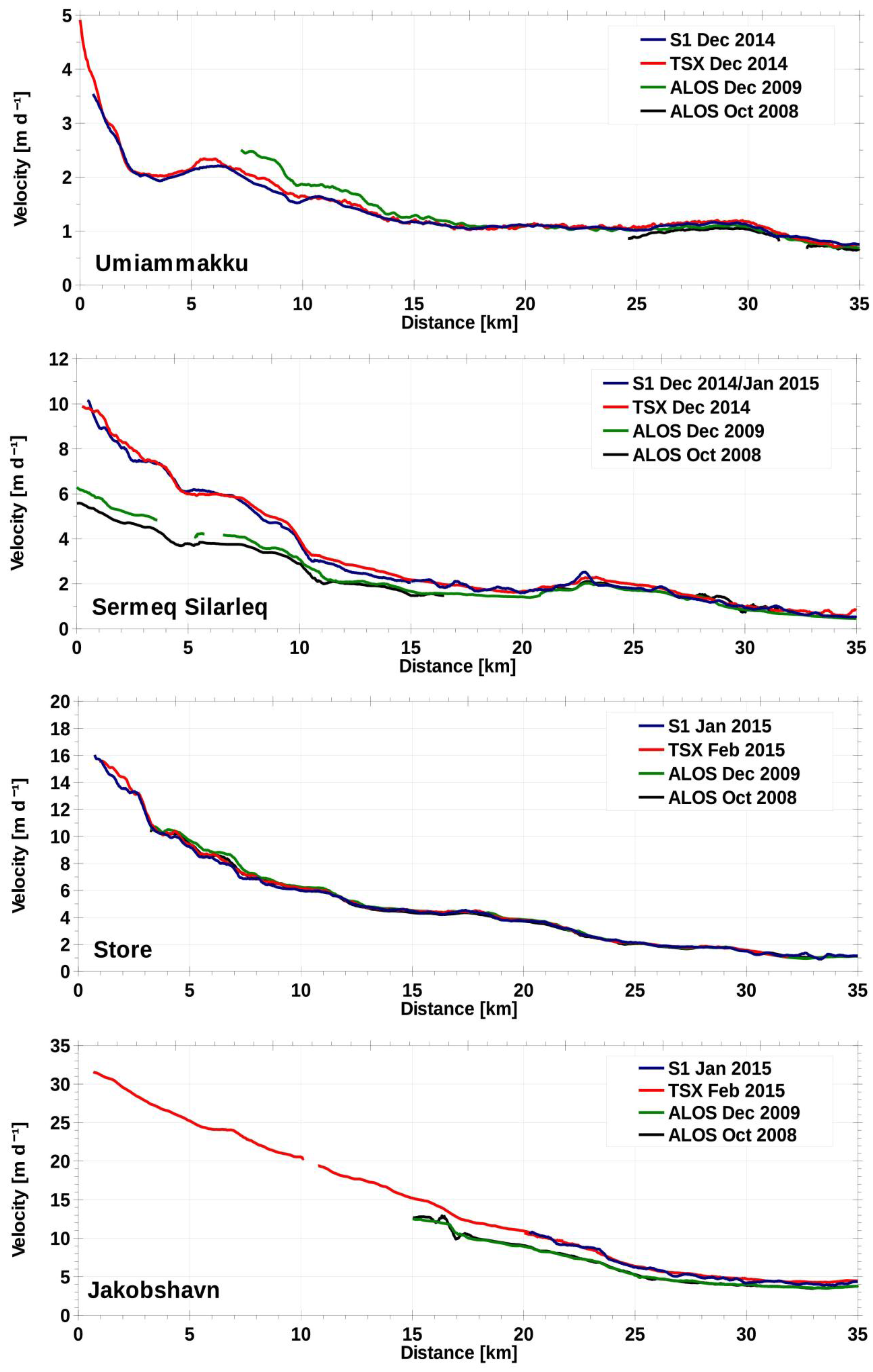
4.2. Comparison with Ice Motion from TerraSAR-X and PALSAR Data


| Glacier | Front Coordinates | Time Span S1 | Time Span TerraSAR-X | Time Span PALSAR |
|---|---|---|---|---|
| Umiammakku Isbrae | 71.727°N 52.397°W | 22. December 2014–3 January 2015 | 12 December 2014–1 January 2015 | 15 September–31 October 2008 20 November 2009–5 January 2010 |
| Sermeq Silarleq | 70.830°N 50.760°W | 0 to 15 km 22 December 2014– 3 January 2015 from 15 to 35 km: 3–15 January 2015 | 16–27 December 2014 | 15 September–31 October 2008 20 November 2009–5 January 2010 |
| Store Gletsjer | 70.378°N 50.611°W | 3–15 January 2015 | 3–14 February 2015 | 15 September–31 October 2008 20 November 2009–5 January 2010 |
| Jakboshavn Isbrae | 69.147°N 49.571°W | 3–15 January 2015 | 8–19 February 2015 | 15 September–31 October 2008 20 November 2009–5 January 2010 |

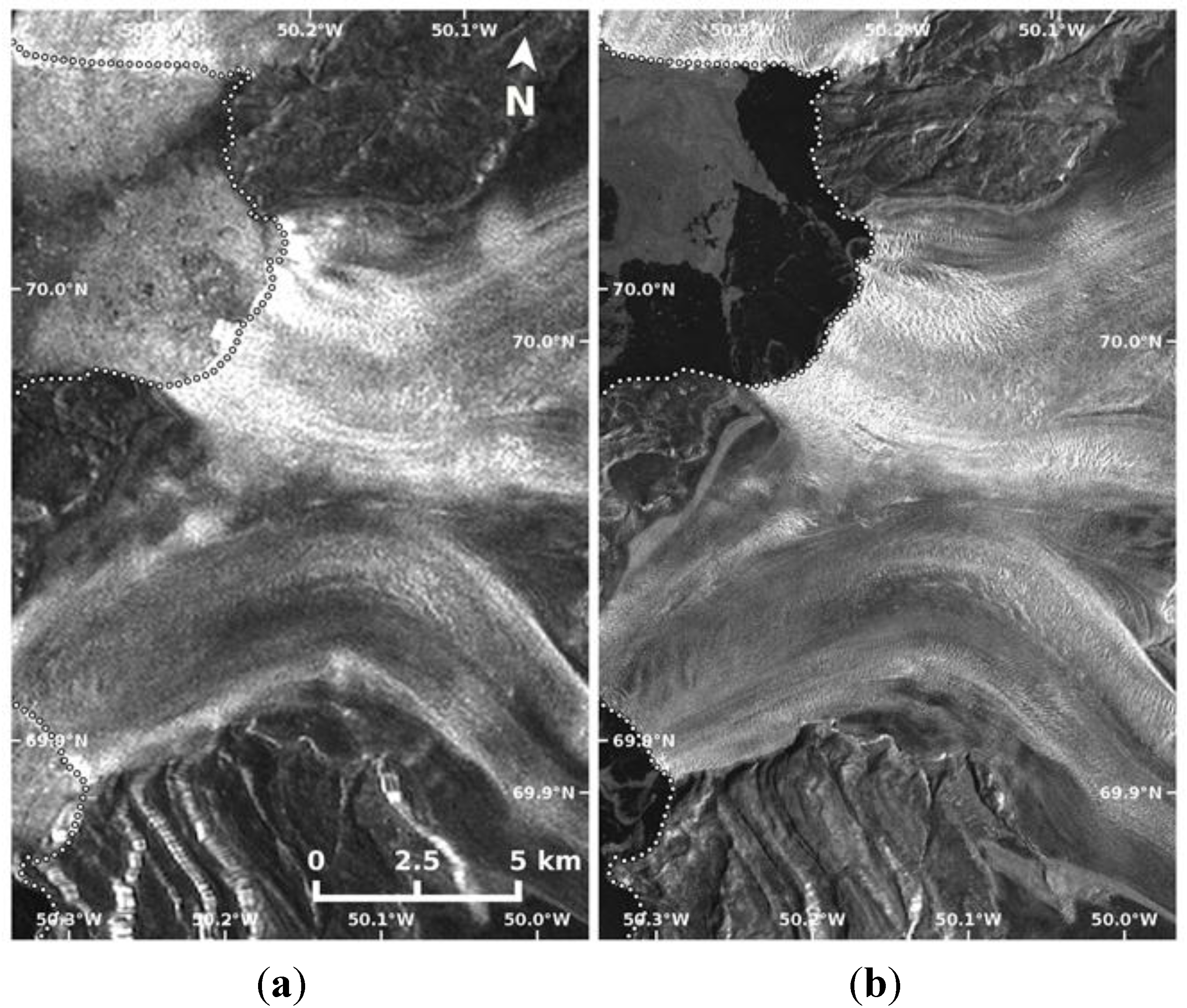
4.3. Error Estimate
- The error introduced during the matching procedure used to determine the offsets of the image templates. This error is related to the degree of correlation between the templates in the different images. It depends on the co-registration of the image pairs, the template size, and on the quality of amplitude features and/or stability of speckle used for tracking.
- Ionospheric disturbances due to fluctuations in ionospheric electron density that are causing phase gradients resulting in azimuth shifts [29]. These are clearly evident as streaks in the retrieved velocity, aligned slightly oblique to the LOS direction.
- Geocoding error. Due to the very precise ephemeris data for S1 the error through transformation from slant range to map projection is primarily caused by height errors in the DEM used for topographic correction.
5. Discussion
6. Conclusions
Acknowledgments
Author Contributions
Conflicts of Interest
References
- Aschbacher, J.; Milagro-Peréz, M.P. The European Earth monitoring (GMES) programme: Status and perspectives. Remote Sens. Environ. 2012, 120, 3–8. [Google Scholar] [CrossRef]
- Berger, M.; Moreno, J.; Johannessen, J.; Levelt, P.; Hanssen, R. ESA’s sentinel missions in support of earth system science. Remote Sens. Environ. 2012, 120, 84–90. [Google Scholar] [CrossRef]
- Malenovský, Z.; Rott, H.; Cihlar, J.; Schaepman, M.E.; García-Santos, G.; Fernandes, R.; Berger, M. Sentinels for science: Potential of Sentinel-1, -2, and -3 missions for scientific observations of ocean, cryosphere, and land. Remote Sens. Environ. 2012, 120, 91–101. [Google Scholar] [CrossRef]
- Potin, P.; Rosich, B.; Roeder, J.; Bargellini, P. Sentinel-1 mission operations concept. In Proceedings of the IEEE IGARSS, Québec, QC, Canada, 13–18 July 2014; pp. 1465–1468.
- Torres, R.; Snoeij, P.; Geudtner, D.; Bibby, D.; Davidson, M.; Attema, E.; Potin, P.; Rommen, B.; Floury, N.; Brown, M.; et al. GMES Sentinel-1 mission. Remote Sens. Environ. 2012, 120, 9–24. [Google Scholar] [CrossRef]
- Geudtner, D.; Torres, R.; Snoeij, P.; Davidson, M.; Rommen, B. Sentinel-1 system capabilities and applications. In Proceedings of the IEEE IGARSS, Québec, QC, Canada, 13–18 July 2014; pp. 1457–1460.
- Howat, I.M.; Joughin, I.R.; Scambos, T.A. Rapid changes in ice discharge from Greenland outlet glaciers. Science 2007, 315, 1559–1561. [Google Scholar] [CrossRef] [PubMed]
- Joughin, I.; Das, S.B.; King, M.A.; Smith, B.E.; Howat, I.M.; Moon, T. Seasonal speed-up along the western flank of the Greenland Ice Sheet. Science 2008, 320, 781–783. [Google Scholar] [CrossRef] [PubMed]
- Van de Wal, R.S.W.; Boot, W.; van den Broeke, M.R.; Smeets, C.J.P.P.; Reijmer, C.H.; Donker, J.J.A.; Oerlemans, J. Large and rapid melt-induced velocity changes in the ablation zone of the Greenland ice sheet. Science 2008, 321, 111–113. [Google Scholar] [CrossRef] [PubMed]
- Wuite, J.; Rott, H.; Hetzenecker, M.; Floricioiu, D.; de Rydt, J.; Gudmundsson, H.G.; Nagler, T.; Kern, M. Evolution of surface velocities and ice discharge of Larsen B outlet glaciers from 1995 to 2013. Cryosphere 2015, 9, 957–969. [Google Scholar] [CrossRef]
- Moon, T.; Joughin, I.; Smith, B.; Howat, I. 21st-century evolution of Greenland outlet glacier velocities. Science 2012, 336, 576–578. [Google Scholar] [CrossRef] [PubMed]
- Rignot, E.; Mouginot, J.; Scheuchl, B. Ice flow of the Antarctic Ice Sheet. Science 2011, 333, 1427–1430. [Google Scholar] [CrossRef] [PubMed]
- Rignot, E.; Mouginot, J. Ice flow in Greenland for the international polar year 2008–2009. Geophys. Res. Lett. 2012, 39, L11501. [Google Scholar] [CrossRef]
- De Zan, F.; Monti Guarnieri, A. TOPSAR: Terrain observation by progressive scans. IEEE Trans. Geosci. Remote Sens. 2006, 44, 2352–2360. [Google Scholar] [CrossRef]
- Rodriguez-Cassola, M.; Prats-Iraola, P.; de Zan, F.; Scheiber, R.; Reigber, A.; Geudtner, D.; Moreira, A. Doppler-related distortions in TOPS SAR images. IEEE Trans. Geosci. Remote Sens. 2015, 53, 25–35. [Google Scholar] [CrossRef]
- Thain, C.; Herbert, C.; Lim, P. Sentinel-1 Product Specification; MDA Document Number: SEN-RS-52-7441, Reference S1-RS-MDA-52-7441; ESA: Frascati, Italy, 2014. [Google Scholar]
- Holzner, J.; Bamler, R. Burst-mode and ScanSAR interferometry. IEEE Trans. Geosci. Remote Sens. 2002, 40, 1917–1934. [Google Scholar] [CrossRef]
- Breit, H.; Fritz, T.; Balss, U.; Lachaise, M.; Niedermeier, A.; Vonavka, M. TerraSAR-X SAR processing and products. IEEE Trans. Geosci. Remote Sens. 2010, 48, 717–727. [Google Scholar] [CrossRef]
- Shimada, M.; Isoguchi, O.; Tadono, T.; Isono, K. PALSAR radiometric and geometric calibration. IEEE Trans. Geosci. Remote Sens. 2009, 47, 3915–3932. [Google Scholar] [CrossRef]
- Strozzi, T.; Luckman, A.; Murray, T.; Wegmüller, U.; Werner, C. Glacier motion estimation using SAR offset-tracking procedures. IEEE Trans. Geosci. Remote Sens. 2002, 40, 2384–2391. [Google Scholar] [CrossRef]
- Rott, H. Advances in interferometric synthetic aperture radar (InSAR) in earth system science. Prog. Phys. Geogr. 2009, 33, 769–791. [Google Scholar] [CrossRef]
- Bamler, R.; Hartl, P. Synthetic aperture radar interferometry. Inverse Probl. 1998, 14, R1–R54. [Google Scholar] [CrossRef]
- Howat, I.M.; Negrete, A.; Smith, B.E. The Greenland Ice Mapping Project (GIMP) land classification and surface elevation datasets. Cryosphere 2014, 8, 1509–1518. [Google Scholar] [CrossRef]
- Sansosti, E.; Berardino, P.; Manunta, M.; Serafino, F.; Fornaro, G. Geometrical SAR image registration. IEEE Trans. Geosci. Remote Sens. 2006, 44, 2861–2870. [Google Scholar] [CrossRef]
- Prats-Iraola, P.; Scheiber, R.; Marotti, L.; Wollstadt, S.; Reigber, A. TOPS interferometry with TerraSAR-X. IEEE Trans. Geosci. Remote Sens. 2012, 50, 3179–3188. [Google Scholar] [CrossRef]
- Miranda, N.; Palumbo, G. Sentinel-1 Instrument and Product Performance Status. Available online: http://seom.esa.int/fringe2015/files/presentation359.pdf (accessed on 11 May 2015).
- Joughin, I.; Smith, B.E.; Howat, I.M.; Scambos, T.; Moon, T. Greenland flow variability from ice-sheet-wide velocity mapping. J. Glaciol. 2010, 56, 415–430. [Google Scholar] [CrossRef]
- Mouginot, J.; Scheuchl, B.; Rignot, E. Mapping of ice motion in Antarctica using synthetic-aperture radar data. Remote Sens. 2012, 4, 2753–2767. [Google Scholar] [CrossRef]
- Gray, A.L.; Mattar, K.E.; Sofko, G. Influence of ionospheric electron density fluctuations on satellite radar interferometry. Geophys. Res. Lett. 2000, 27, 1451–1454. [Google Scholar] [CrossRef]
- Joughin, I.; Smith, B.E.; Shean, D.E.; Floricioiu, D. Brief communication: Further summer speedup of Jakobshavn Isbræ. Cryosphere 2014, 8, 209–214. [Google Scholar] [CrossRef]
- Moon, T.; Joughin, I.; Smith, B.; van den Broeke, M.R.; van de Berg, W.J.; Noël, B.; Usher, M. Distinct patterns of seasonal Greenland glacier velocity. Geophys. Res. Lett. 2014, 41, 7209–7216. [Google Scholar] [CrossRef] [PubMed]
- Joughin, I.; Smith, B.E.; Howat, I.M.; Floricioiu, D.; Alley, R.B.; Truffer, M.; Fahnestock, M. Seasonal to decadal scale variations in the surface velocity of Jakobshavn Isbrae, Greenland: Observation and model-based analysis. J. Geophys. Res. 2012, 117. [Google Scholar] [CrossRef]
- Csatho, B.M.; Schenk, A.F.; van der Veen, C.J.; Babonis, G.; Duncan, K.; Rezvanbehbahani, S.; van den Broeke, M.R.; Simonsen, S.B.N.; Nagarajan, S.; van Angelen, J.H. Laser altimetry reveals complex pattern of Greenland Ice Sheet dynamics. Proc. Natl. Acad. Sci. USA 2014, 111, 18478–18483. [Google Scholar] [CrossRef] [PubMed]
- Ahlstrøm, A.P.; Andersen, S.B.; Andersen, M.L.; Machguth, H.; Nick, F.M.; Joughin, I.; Reijmer, C.H.; van de Wal, R.; Boncori, J.P.; Box, J.E. Seasonal velocities of eight major marine-terminating outlet glaciers of the Greenland ice sheet from continuous in situ GPS instrument. Earth Syst. Sci. Data 2013, 5. [Google Scholar] [CrossRef]
- ESA. The Changing Earth-New Scientific Challenges for ESA’s Living Planet Programme; ESA SP-1304; ESA: Frascati, Italy, 2006; Available online: http://www.esa.int/esaMI/ESA_Publications/SEMAJUB474F_0.html (accessed on 17 July 2015).
- Drusch, M.; Del Bello, U.; Carlier, S.; Colin, O.; Fernandez, V.; Gascon, F.; Hoersch, B.; Isola, C.; Laberinti, P.; Martimort, P.; et al. Sentinel-2: ESA’s optical high-resolution mission for GMES operational services. Remote Sens. Environ. 2012, 120, 25–36. [Google Scholar] [CrossRef]
- Donlon, C.; Berruti, B.; Buongiorno, A.; Ferreira, M.-H.; Féménias, P.; Frerick, J.; Goryl, P.; Klein, U.; Laur, H.; Mavrocordatos, C.; et al. The Global Monitoring for Environment and Security (GMES) Sentinel-3 mission. Remote Sens. Environ. 2012, 120, 37–57. [Google Scholar] [CrossRef]
© 2015 by the authors; licensee MDPI, Basel, Switzerland. This article is an open access article distributed under the terms and conditions of the Creative Commons Attribution license (http://creativecommons.org/licenses/by/4.0/).
Share and Cite
Nagler, T.; Rott, H.; Hetzenecker, M.; Wuite, J.; Potin, P. The Sentinel-1 Mission: New Opportunities for Ice Sheet Observations. Remote Sens. 2015, 7, 9371-9389. https://doi.org/10.3390/rs70709371
Nagler T, Rott H, Hetzenecker M, Wuite J, Potin P. The Sentinel-1 Mission: New Opportunities for Ice Sheet Observations. Remote Sensing. 2015; 7(7):9371-9389. https://doi.org/10.3390/rs70709371
Chicago/Turabian StyleNagler, Thomas, Helmut Rott, Markus Hetzenecker, Jan Wuite, and Pierre Potin. 2015. "The Sentinel-1 Mission: New Opportunities for Ice Sheet Observations" Remote Sensing 7, no. 7: 9371-9389. https://doi.org/10.3390/rs70709371