
Estimation of Surface Soil Moisture from Thermal Infrared Remote Sensing Using an Improved Trapezoid Method


Abstract
:
1. Introduction
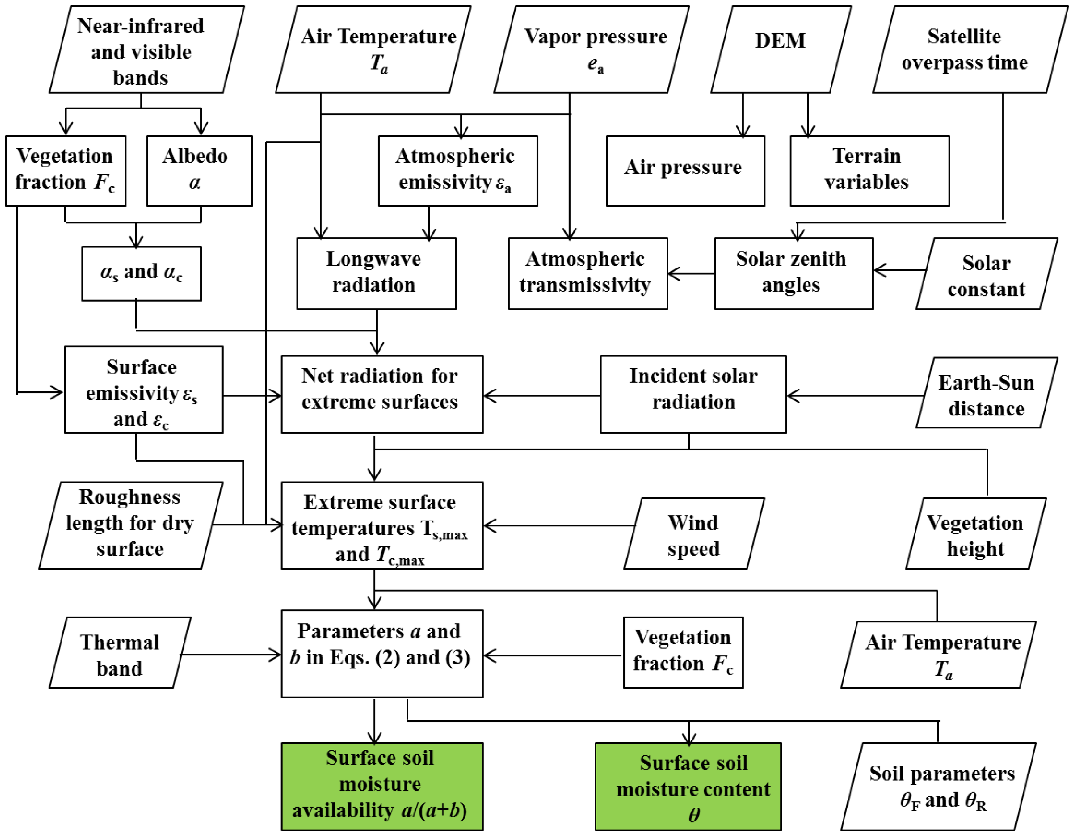
2. Methodology
2.1. Trapezoidal VI/LST Space
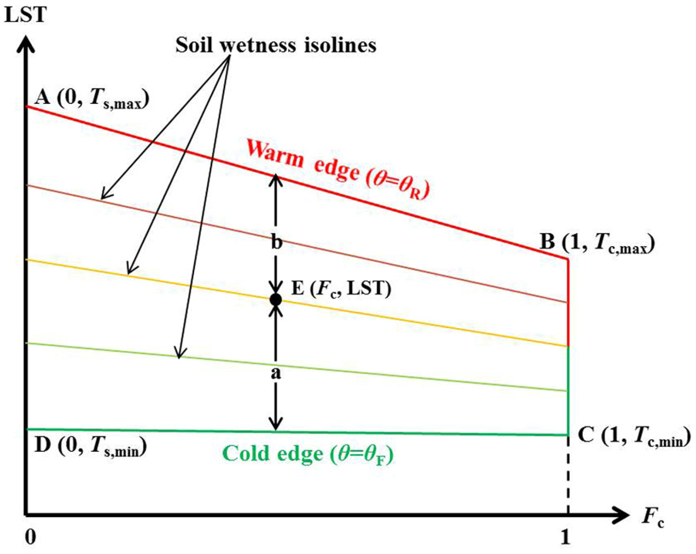
2.2. Determination of Boundaries
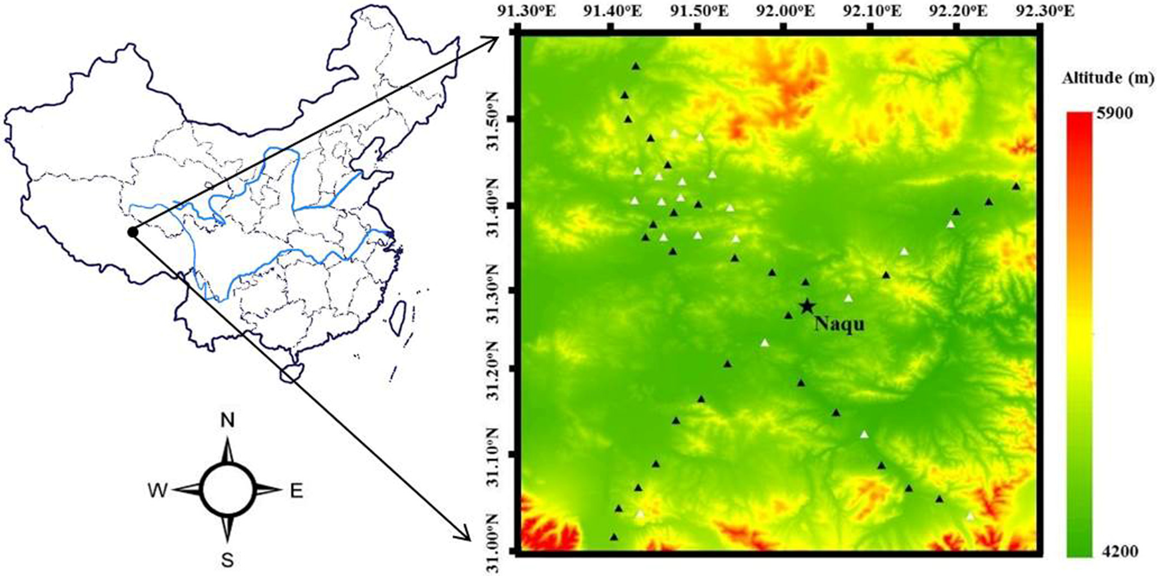
3. Study Area and Data
3.1. Site Description and SM Measurement
3.2. Remote Sensing Data
3.3. Other Data Sources
4. Results and Discussion
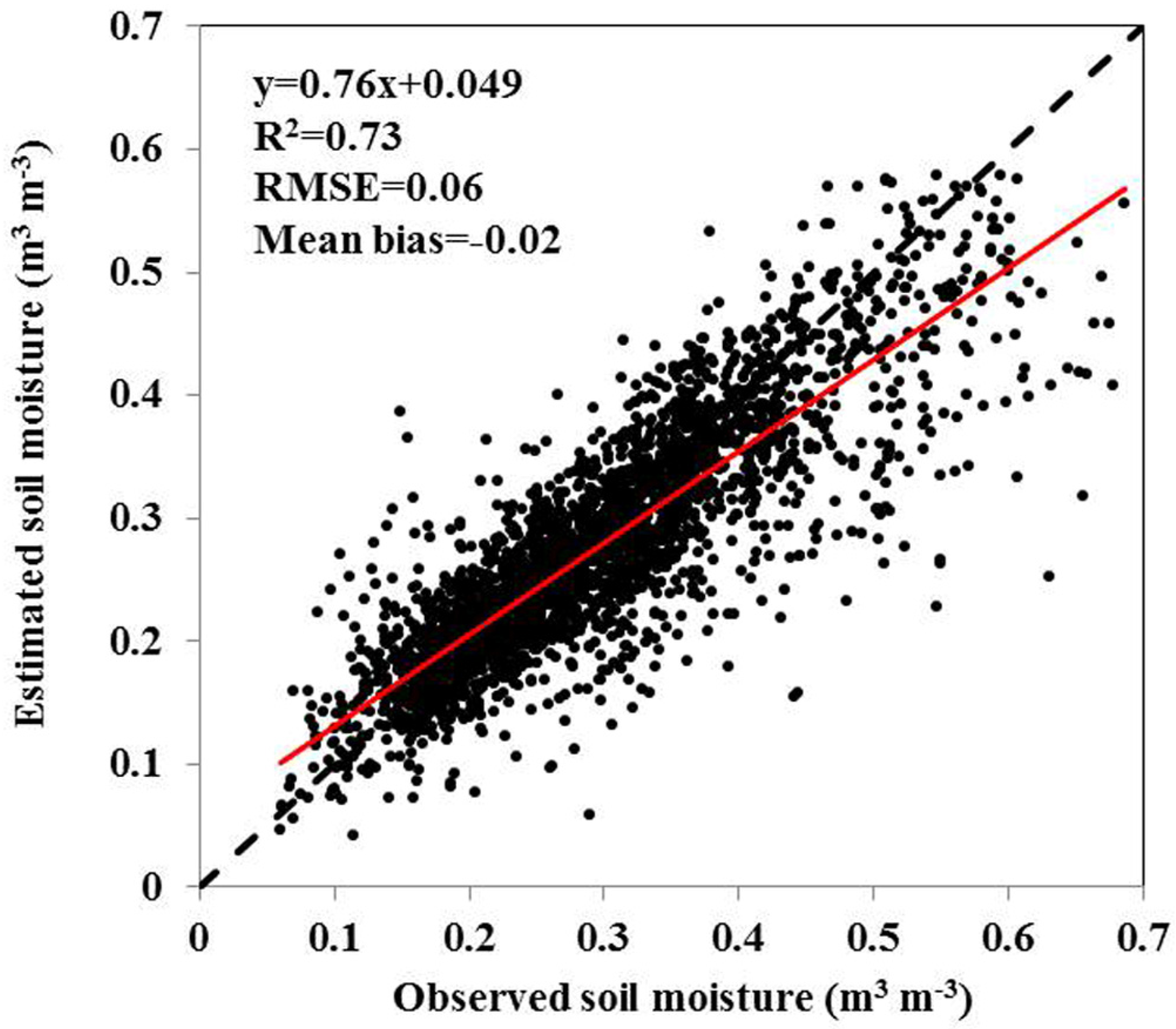
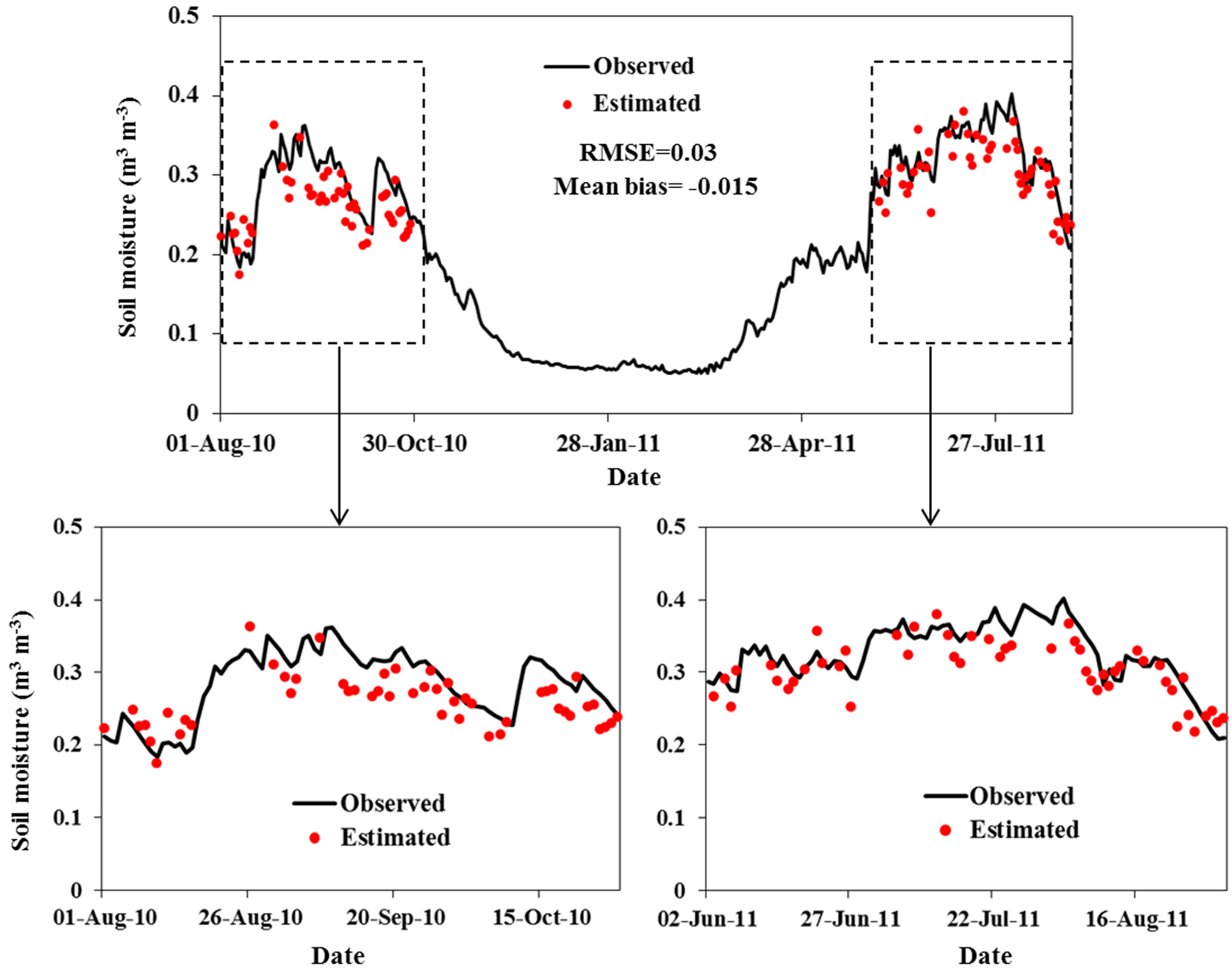
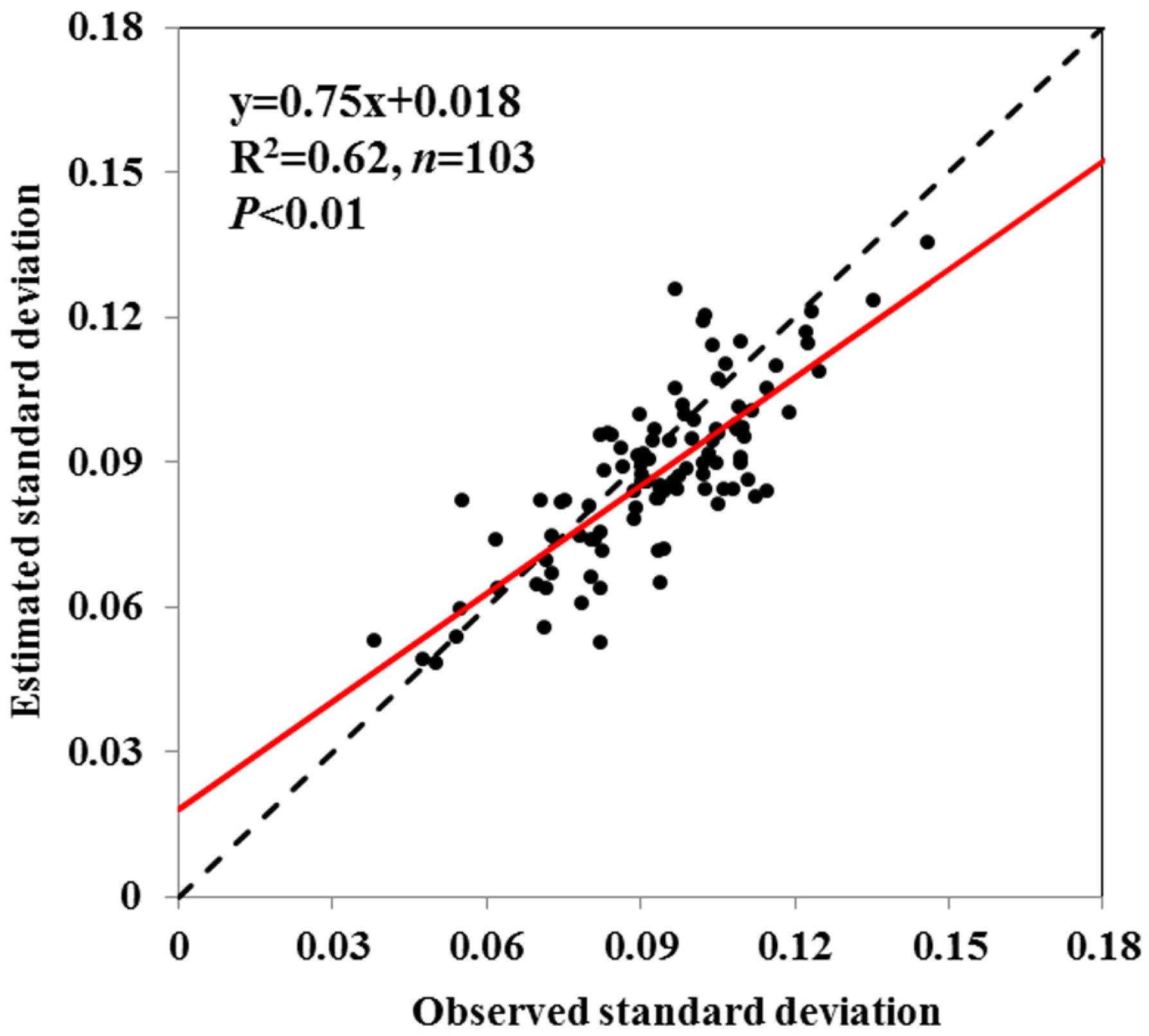
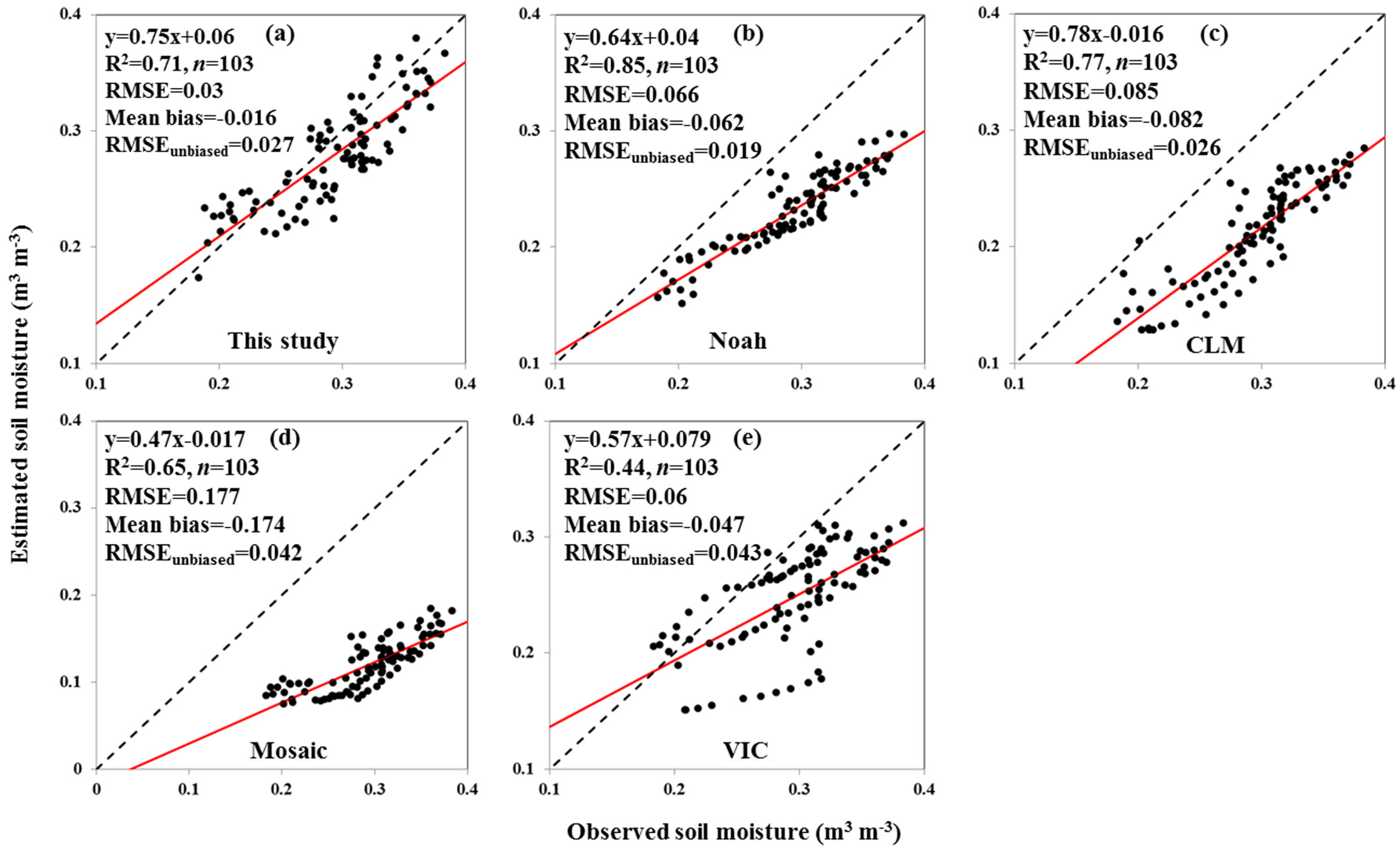
4.1. Validation with Site Observations
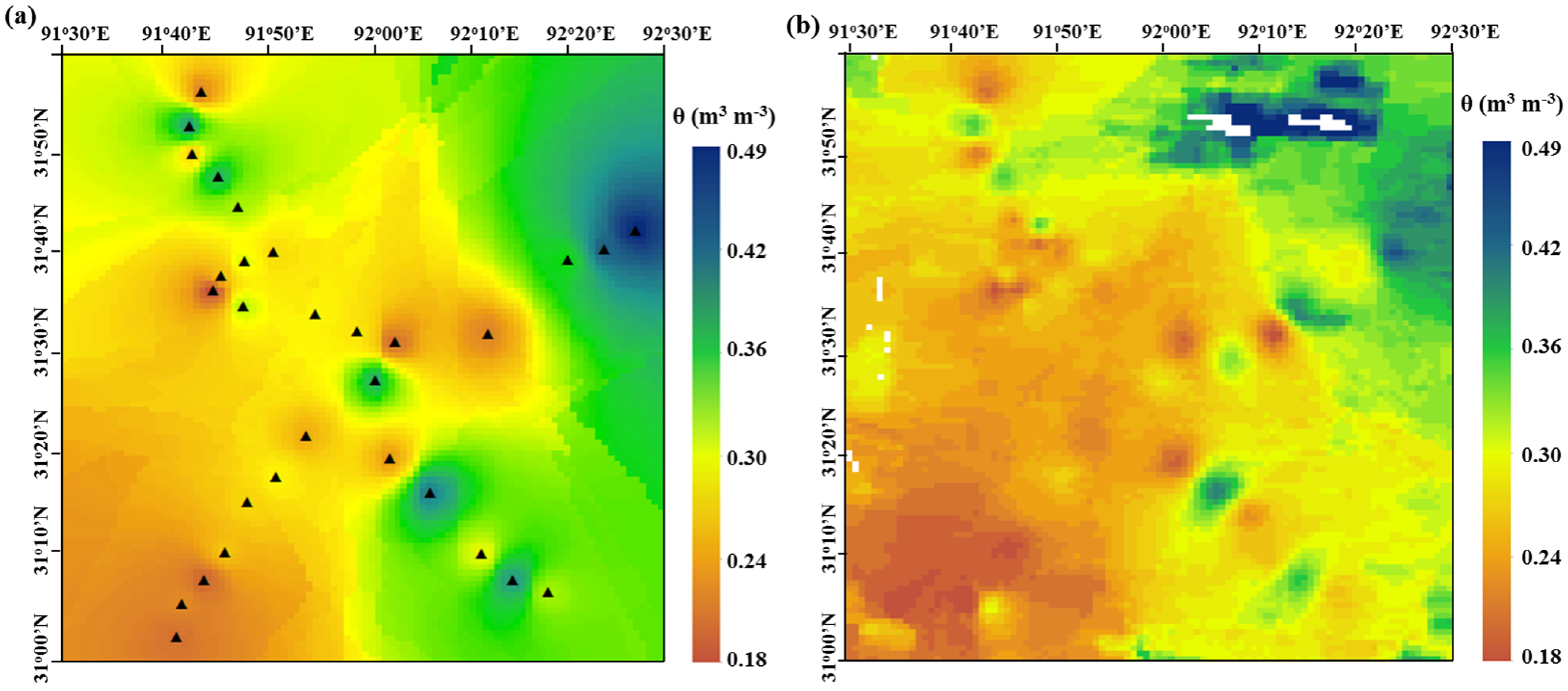
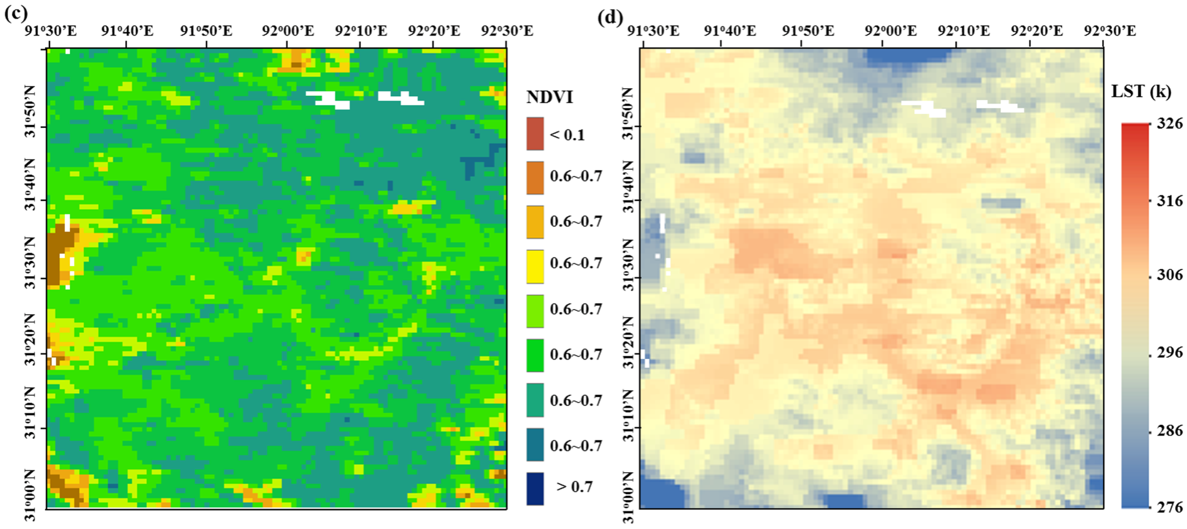
4.2. Spatial Distribution of Soil Moisture


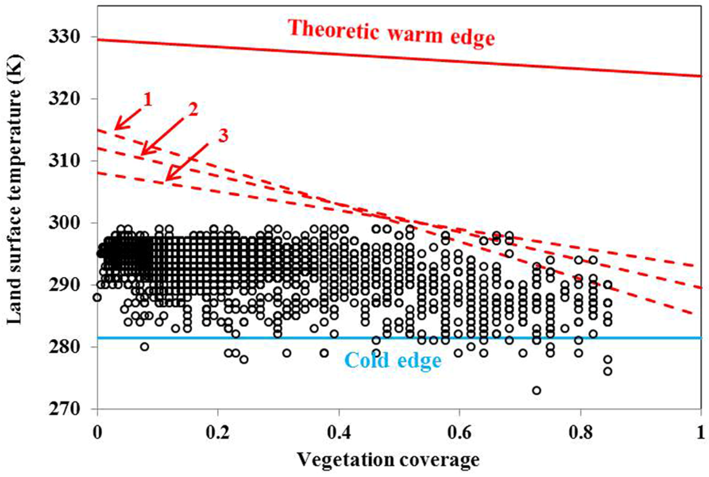
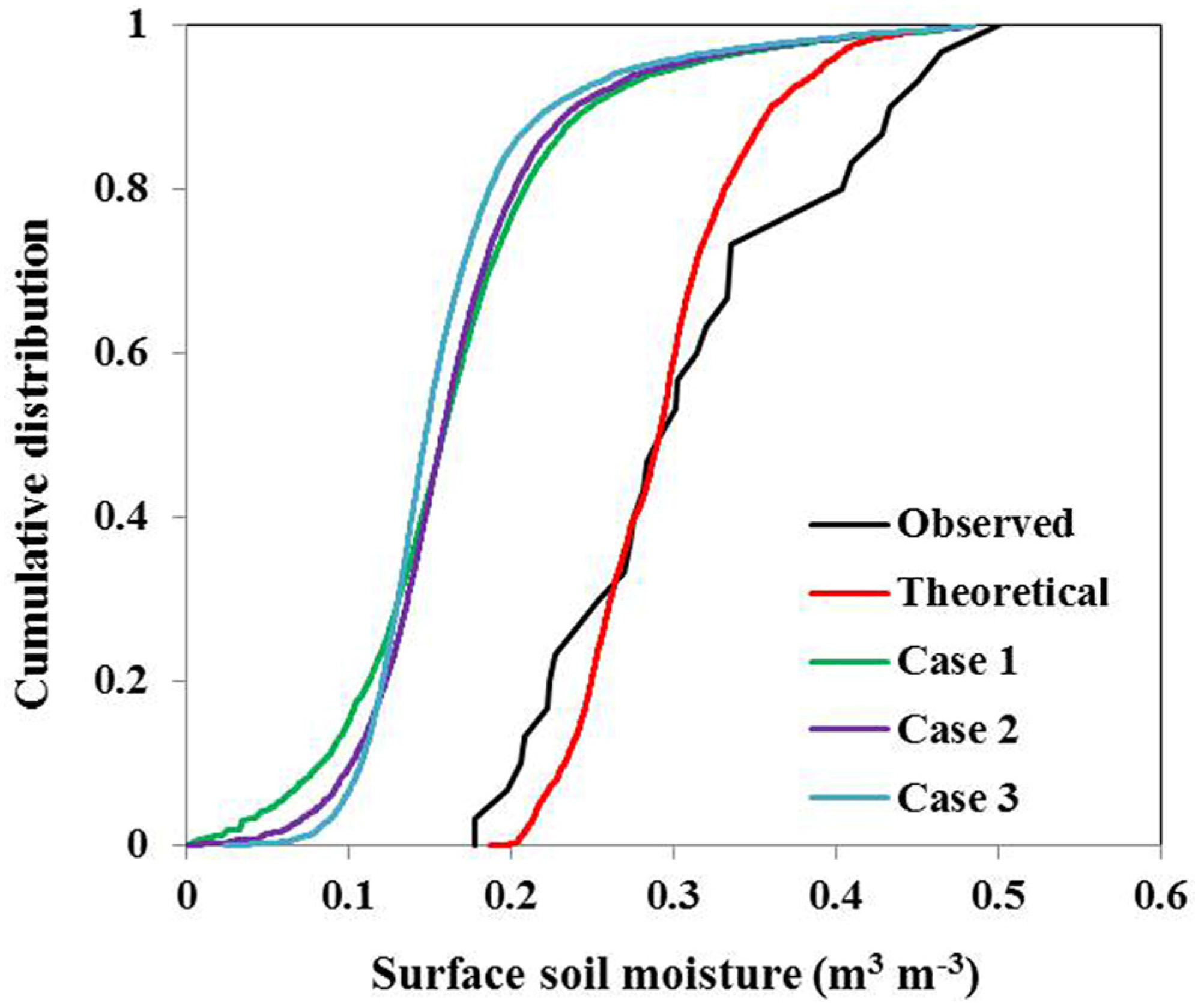
4.3. Theoretic Boundary vs. Observed Boundary


| Surface SM | Mean | Stand Deviation | CV | RMSE | Mean Bias | R2 |
|---|---|---|---|---|---|---|
| Observed | 0.31 | 0.087 | 0.28 | - | - | - |
| Theoretical | 0.29 | 0.074 | 0.26 | 0.05 | −0.02 | 0.86 |
| Case 1 | 0.17 | 0.073 | 0.43 | 0.18 | −0.14 | 0.42 |
| Case 2 | 0.17 | 0.070 | 0.41 | 0.18 | −0.14 | 0.46 |
| Case 3 | 0.16 | 0.062 | 0.39 | 0.19 | −0.15 | 0.54 |
4.4. Sensitivity Analysis
| Variation (%/K) | −20(−2) | −15(−1.5) | −10(−1) | −5(−0.5) | 5(0.5) | 10(1) | 15(1.5) | 20(2) |
|---|---|---|---|---|---|---|---|---|
| LST | 6.06 | 4.56 | 3.03 | 1.53 | −1.50 | −3.03 | −4.56 | −6.06 |
| Ta | −5.22 | −3.94 | −2.65 | −1.32 | 1.36 | 2.72 | 4.08 | 5.43 |
| u | 3.38 | 2.72 | 1.85 | 0.94 | −0.91 | −1.85 | −2.79 | −3.76 |
| αc_max | 0.49 | 0.38 | 0.24 | 0.14 | −0.10 | −0.24 | −0.35 | −0.49 |
| αs_max | 2.33 | 1.78 | 1.22 | 0.63 | −0.73 | −1.25 | −1.95 | −2.65 |
| ea | 0.21 | 0.17 | 0.10 | 0.07 | −0.03 | −0.10 | −0.14 | −0.17 |
| θF | −19.02 | −14.29 | −9.52 | −4.73 | 4.75 | 9.57 | 14.32 | 19.08 |
| θR | −0.54 | −0.41 | −0.28 | −0.14 | 0.14 | 0.28 | 0.41 | 0.54 |
| NDVImax | −1.43 | −0.94 | −0.56 | −0.24 | 0.21 | 0.38 | 0.56 | 0.66 |
| NDVImin | −0.03 | −0.03 | 0.00 | 0.00 | 0.03 | 0.03 | 0.07 | 0.07 |
| n | −0.35 | −0.24 | −0.14 | −0.07 | 0.10 | 0.17 | 0.24 | 0.31 |
4.5. Comparison with Land Surface Models

5. Conclusions
Acknowledgment
Author Contributions
Conflicts of Interest
References
- Seneviratne, S.I.; Corti, T.; Davin, E.L.; Hirschi, M.; Jaeger, E.B.; Lehner, I.; Orlowsky, B.; Teuling, A.J. Investigating soil moisture–climate interactions in a changing climate: A review. Earth-Sci. Rev. 2010, 99, 125–161. [Google Scholar] [CrossRef]
- Wood, E.F. Effects of soil moisture aggregation on surface evaporative fluxes. J. Hydrol. 1997, 190, 397–412. [Google Scholar] [CrossRef]
- Entekhabi, D.; Njoku, E.G.; O’Neill, P.E.; Kellogg, K.H.; Crow, W.T.; Edelstein, W.N.; Entin, J.K.; Goodman, S.D.; Jackson, T.J.; Johnson, J.; et al. The soil moisture active passive (SMAP) mission. Proc. IEEE 2010, 98, 704–716. [Google Scholar] [CrossRef]
- McCabe, M.F.; Gao, H.; Wood, E.F. Evaluation of AMSR-E-derived soil moisture retrievals using ground-based and PSR airborne data during SMEX02. J. Hydrometeorol. 2005, 6, 864–877. [Google Scholar] [CrossRef]
- Wanger, W.; Bloschi, G.; Pampaloni, P.; Calvet, J.; Bizzarri, B.; Wigneron, J.P.; Kerr, Y. Operational readiness of microwave remote sensing of soil moisture for hydrologic applications. Nord. Hydrol. 2007, 38, 1–20. [Google Scholar]
- Kerr, Y.H.; Waldteufel, P.; Wigneron, J.P.; Martinuzzi, J.; Font, J.; Berger, M. Soil moisture retrieval from space: The soil moisture and ocean salinity (SMOS) mission. IEEE Trans.Geosci. Remote Sens. 2001, 39, 1729–1735. [Google Scholar] [CrossRef]
- Gruhier, C.; de Rosnay, P.; Hasenauer, S.; Holmes, T.; de Jeu, R.; Kerr, Y.; Mougin, E.; Njoku, E.; Timouk, F.; Wagner, W.; et al. Soil moisture active and passive microwave products: Intercomparison and evaluation over a sahelian site. Hydrol. Earth Syst. Sci. 2010, 14, 141–156. [Google Scholar] [CrossRef]
- Schmugge, T.J. Remote Sensing of Soil Moisture; Wiley: New York, NY, USA, 1985. [Google Scholar]
- Merlin, O.; Al Bitar, A.; Walker, J.P.; Kerr, Y. An improved algorithm for disaggregating microwave-based soil moisture based on red, near-infrared and thermal infrared data. Remote Sens. Environ. 2010, 114, 2305–2316. [Google Scholar] [CrossRef] [Green Version]
- Anderson, M.C.; Norman, J.M.; Mecikalski, J.R.; Otkin, J.A.; Kustas, W.P. A climatological study of evapotranspiration and moisture stress across the continental united states based on thermal remote sensing: 1. Model formulation. J. Geophys. Res.: Atmos. 2007, 112, D10117. [Google Scholar] [CrossRef]
- Carlson, T.N. An overview of the “triangle method” for estimating surface evapotranspiration and soil moisture from satellite imagery. Sensors 2007, 7, 1612–1629. [Google Scholar] [CrossRef]
- Long, D.; Singh, V.P.; Scanlon, B.R. Deriving theoretical boundaries to address scale dependencies of triangle models for evapotranspiration estimation. J. Geophys. Res.: Atmos. 2012, 117, D05113. [Google Scholar] [CrossRef]
- Yang, Y.; Shang, S. A hybrid dual-source scheme and trapezoid framework–based evapotranspiration model (HTEM) using satellite images: Algorithm and model test. J. Geophys. Res.: Atmos. 2013, 118, 2284–2300. [Google Scholar] [CrossRef]
- Zhang, R.H.; Sun, X.M.; Wang, X.M.; Xu, J.P.; Zhu, Z.L.; Tian, J. An operational two-layer remote sensing model to estimate surface flux in regional scale: Physical background. Sci. China Ser. D 2005, 48, 225–244. [Google Scholar]
- Yang, Y.; Scott, R.L.; Shang, S. Modeling evapotranspiration and its partitioning over a semiarid shrub ecosystem from satellite imagery: A multiple validation. J. Appl. Remote Sens. 2013, 7. [Google Scholar] [CrossRef]
- Carlson, T.N.; Gillies, R.R.; Perry, E.M. A method to make use of thermal infrared temperature and NDVI measurements to infer surface soil water content and fractional vegetation cover. Remote Sens. Rev. 1994, 9, 161–173. [Google Scholar] [CrossRef]
- Gillies, R.R.; Carlson, T.N. Thermal remote sensing of surface soil water content with partial vegetation cover for incorporation into climate models. J. Appl. Meteorol. 1995, 34, 745–756. [Google Scholar] [CrossRef]
- Moran, M.S.; Clarke, T.R.; Inoue, Y.; Vidal, A. Estimating crop water deficit using the relation between surface-air temperature and spectral vegetation index. Remote Sens. Environ. 1994, 49, 246–263. [Google Scholar] [CrossRef]
- Choi, M.; Kustas, W.P.; Anderson, M.C.; Allen, R.G.; Li, F.; Kjaersgaard, J.H. An intercomparisonof three remote sensing-based surface energy balance algorithms over a corn and soybean production region (Iowa, U.S.) during smacex. Agric. For. Meteorol. 2009, 149, 2082–2097. [Google Scholar] [CrossRef]
- Stisen, S.; Sandholt, I.; Nørgaard, A.; Fensholt, R.; Jensen, K.H. Combining the triangle method with thermal inertia to estimate regional evapotranspiration—Applied to MSG-SEVIRI data in the Senegal River Basin. Remote Sens. Environ. 2008, 112, 1242–1255. [Google Scholar] [CrossRef]
- Yang, Y.; Long, D.; Guan, H.; Liang, W.; Simmons, C.; Batelaan, O. Comparison of three dual-sourceremote sensing evapotranspiration models during the MUSOEXE-12 campaign: Revisit of model physics. Water Resour. Res. 2015, 51, 3145–3165. [Google Scholar] [CrossRef]
- Yang, K.; Qin, J.; Zhao, L.; Chen, Y.; Tang, W.; Han, M.; Lazhu; Chen, Z.; Lv, N.; Ding, B.; et al. A multiscale soil moisture and freeze–thaw monitoring network on the third pole. Bull. Am. Meteorol. Soc. 2013, 94, 1907–1916. [Google Scholar] [CrossRef]
- Rodell, M.; Houser, P.R.; Jambor, U.; Gottschalck, J.; Mitchell, K.; Meng, C.J.; Arsenault, K.; Cosgrove, B.; Radakovich, J.; Bosilovich, M.; et al. The global land data assimilation system. Bull. Am. Meteorol. Soc. 2004, 85, 381–394. [Google Scholar] [CrossRef]
- Allen, R.G.; Pereira, L.S.; Raes, D.; Smith, M. Crop Evapotranspiration-Guidelines for Computing Crop Water Requirement; United Nations Food and Agriculture Organization: Rome, Italy, 1998. [Google Scholar]
- Tasumi, M. Progress in Operational Estimation of Regional Evapotranspiration Using Satellite Imagery; University of Idaho: Moscow, ID, USA, 2003. [Google Scholar]
- Brutsaert, W. On a derivable formula for long-wave radiation from clear skies. Water Resour. Res. 1975, 11, 742–744. [Google Scholar] [CrossRef]
- Sánchez, J.M.; Kustas, W.P.; Caselles, V.; Anderson, M.C. Modelling surface energy fluxes over maize using a two-source patch model and radiometric soil and canopy temperature observations. Remote Sens. Environ. 2008, 112, 1130–1143. [Google Scholar] [CrossRef]
- Long, D.; Singh, V.P. A two-source trapezoid model for evapotranspiration (TTME) from satellite imagery. Remote Sens. Environ. 2012, 121, 370–388. [Google Scholar] [CrossRef]
- Campbell, G.S.; Norman, J.M. Introduction to Environmental Biophysics; Springer: New York, NY, USA, 1998. [Google Scholar]
- Qin, J.; Yang, K.; Lu, N.; Chen, Y.; Zhao, L.; Han, M. Spatial upscaling of insitu soil moisture measurements based on MODIS-derived apparent thermal inertia. Remote Sens. Environ. 2013, 138, 1–9. [Google Scholar] [CrossRef]
- Chen, Y.; Yang, K.; Tang, W.; Qin, J.; Zhao, L. Parameterizing soil organic carbon’s impacts on soil porosity and thermal parameters for eastern Tibet Grasslands. Sci. China Earth Sci. 2012, 55, 1001–1011. [Google Scholar] [CrossRef]
- Zhao, L.; Yang, K.; Qin, J.; Chen, Y.; Tang, W.; Montzka, C.; Wu, H.; Lin, C.; Han, M.; Vereecken, H. Spatiotemporal analysis of soil moisture observations within a Tibetan Mesoscale Area and its implication to regional soil moisture measurements. J. Hydrol. 2013, 482, 92–104. [Google Scholar] [CrossRef]
- NASA Data Center. Available online: http://reverb.echo.nasa.gov (accessed on 19 June 2015).
- Liang, S.L. Narrowband to broadband conversions of land surface albedo I algorithms. Remote Sens. Environ. 2001, 76, 213–238. [Google Scholar] [CrossRef]
- Huete, A.; Didan, K.; Miura, T.; Rodriguez, E.P.; Gao, X.; Ferreira, L.G. Overview of the radiometric and biophysical performance of the MODIS vegetation indices. Remote Sens. Environ. 2002, 83, 195–213. [Google Scholar] [CrossRef]
- Donohue, R.J.; Roderick, M.L.; McVicar, T.R.; Farquar, G.D. Impact of CO2 fertilization on maximum foliage cover across the globe's warm, arid environments. Geophys. Res. Lett. 2013, 40, 3031–3035. [Google Scholar] [CrossRef]
- Choudhury, B.J.; Ahmed, N.U.; Idso, S.B.; Reginato, R.J.; Daughtry, C.S.T. Relations between evaporation coefficients and vegetation indices studied by model simulations. Remote Sens. Environ. 1994, 50, 1–17. [Google Scholar] [CrossRef]
- Zhou, X.; Guan, H.; Xie, H.; Wilson, J.L. Analysis and optimization of NDVI definitions and areal fraction models in remote sensing of vegetation. Int. J. Remote Sens. 2009, 30, 721–751. [Google Scholar] [CrossRef]
- China Meteorology Data Center. Available online: http://data.cma.gov.cn/ (accessed on 19 June 2015).
- Shuttle Radar Topography Mission. Available online: http://srtm.csi.cginar.org/ (accessed on 19 June 2015).
- Yang, K.; Qin, J.; Guo, X.; Zhou, D.; Ma, Y. Method development for estimating sensible heat flux over the Tibetan Plateau from CMA data. J. Appl. Meteorol. Climatol. 2009, 48, 2474–2486. [Google Scholar] [CrossRef]
- Haise, H.R.; Haas, H.J.; Jensen, L.R. Soil moisture studies of some great plains soils: II. Field capacity as related to 1/3-atmosphere percentage, and “minimum point” as related to 15- and 26-atmosphere percentages1. Soil Sci. Soc. Am. J. 1955, 19, 20–25. [Google Scholar] [CrossRef]
- Lei, Z.D.; Yang, S.X.; Xie, S.C. Soil Water Dynamics; Tsinghua University Press: Beijing, China, 1988. [Google Scholar]
- Schaap, M.G.; Leij, F.J.; van Genuchten, M.T. Neural network analysis for hierarchical prediction of soil hydraulic properties. Soil Sci. Soc. Am. J. 1998, 62, 847–855. [Google Scholar] [CrossRef]
- Ek, M.B.; Mitchell, K.E.; Lin, Y.; Rogers, E.; Grunmann, P.; Koren, V.; Gayno, G.; Tarpley, J.D. Implementation of noah land surface model advances in the national centers for environmental prediction operational mesoscale eta model. J. Geophys. Res.: Atmos. 2003, 108, 8851. [Google Scholar] [CrossRef]
- Koster, R.D.; Suarez, M.J. The components of a SVAT scheme and their effects on a GCMS hydrological cycle. Adv. Water Resour. 1994, 17, 61–78. [Google Scholar] [CrossRef]
- Liang, X.; Lettenmaier, D.P.; Wood, E.F.; Burges, S.J. A simple hydrologically based model of land surface water and energy fluxes for general circulation models. J. Geophys. Res.: Atmos. 1994, 99, 14415–14428. [Google Scholar] [CrossRef]
- Dai, Y.; Zeng, X.; Dickinson, R.E.; Baker, I.; Bonan, G.B.; Bosilovich, M.G.; Denning, A.S.; Dirmeyer, P.A.; Houser, P.R.; Niu, G.; et al. The common land model. Bull. Am. Meteorol. Soc. 2003, 84, 1013–1023. [Google Scholar] [CrossRef]
- Yang, Y.; Shang, S.; LI, C. Correcting the smoothing effect of ordinary kriging estimates in soil moisture interpolation. Adv. Water Sci. 2010, 21, 208–213. [Google Scholar]
- Su, C.-H.; Ryu, D.; Young, R.I.; Western, A.W.; Wagner, W. Inter-comparison of microwave satellite soil moisture retrievals over the murrumbidgee basin, southeast australia. Remote Sens. Environ. 2013, 134, 1–11. [Google Scholar] [CrossRef]
- Chen, Y.; Yang, K.; Qin, J.; Zhao, L.; Tang, W.; Han, M. Evaluation of AMSR-E retrievals and GLDAS simulations against observations of a soil moisture network on the central Tibetan Plateau. J. Geophys. Res.: Atmos. 2013, 118, 4466–4475. [Google Scholar] [CrossRef]
- Long, D.; Scanlon, B.R.; Longuevergne, L.; Sun, A.Y.; Fernando, D.N.; Save, H. Grace satellite monitoring of large depletion in water storage in response to the 2011 drought in Texas. Geophys. Res. Lett. 2013, 40, 3395–3401. [Google Scholar] [CrossRef] [Green Version]
- Long, D.; Longuevergne, L.; Scanlon, B.R. Global analysis of approaches for deriving total water storage changes from grace satellites. Water Resour. Res. 2015, 51, 2574–2594. [Google Scholar] [CrossRef]
- Long, D.; Longuevergne, L.; Scanlon, B.R. Uncertainty in evapotranspiration from land surface modeling, remote sensing, and grace satellites. Water Resour. Res. 2014, 50, 1131–1151. [Google Scholar] [CrossRef]
© 2015 by the authors; licensee MDPI, Basel, Switzerland. This article is an open access article distributed under the terms and conditions of the Creative Commons Attribution license (http://creativecommons.org/licenses/by/4.0/).
Share and Cite
Yang, Y.; Guan, H.; Long, D.; Liu, B.; Qin, G.; Qin, J.; Batelaan, O. Estimation of Surface Soil Moisture from Thermal Infrared Remote Sensing Using an Improved Trapezoid Method. Remote Sens. 2015, 7, 8250-8270. https://doi.org/10.3390/rs70708250
Yang Y, Guan H, Long D, Liu B, Qin G, Qin J, Batelaan O. Estimation of Surface Soil Moisture from Thermal Infrared Remote Sensing Using an Improved Trapezoid Method. Remote Sensing. 2015; 7(7):8250-8270. https://doi.org/10.3390/rs70708250
Chicago/Turabian StyleYang, Yuting, Huade Guan, Di Long, Bing Liu, Guanghua Qin, Jun Qin, and Okke Batelaan. 2015. "Estimation of Surface Soil Moisture from Thermal Infrared Remote Sensing Using an Improved Trapezoid Method" Remote Sensing 7, no. 7: 8250-8270. https://doi.org/10.3390/rs70708250