
Mapping Priorities to Focus Cropland Mapping Activities: Fitness Assessment of Existing Global, Regional and National Cropland Maps


Abstract
:
1. Introduction
2. Materials
2.1. Land Cover and Cropland Maps
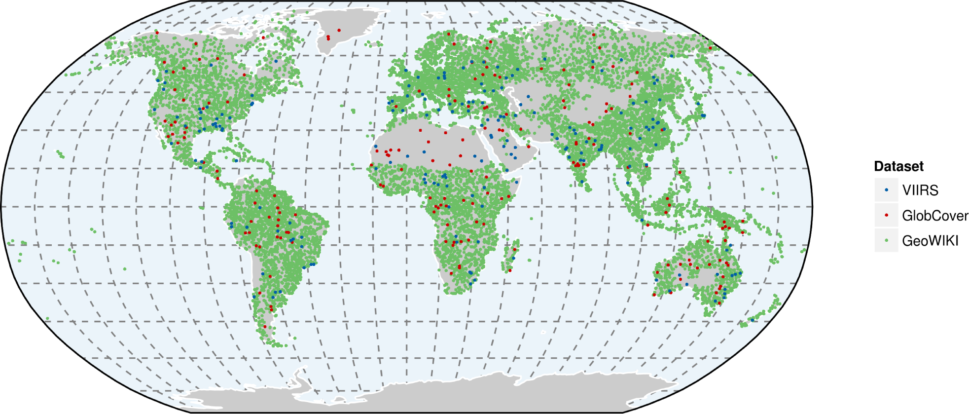
2.2. Global Validation Datasets
2.3. Ancillary Data
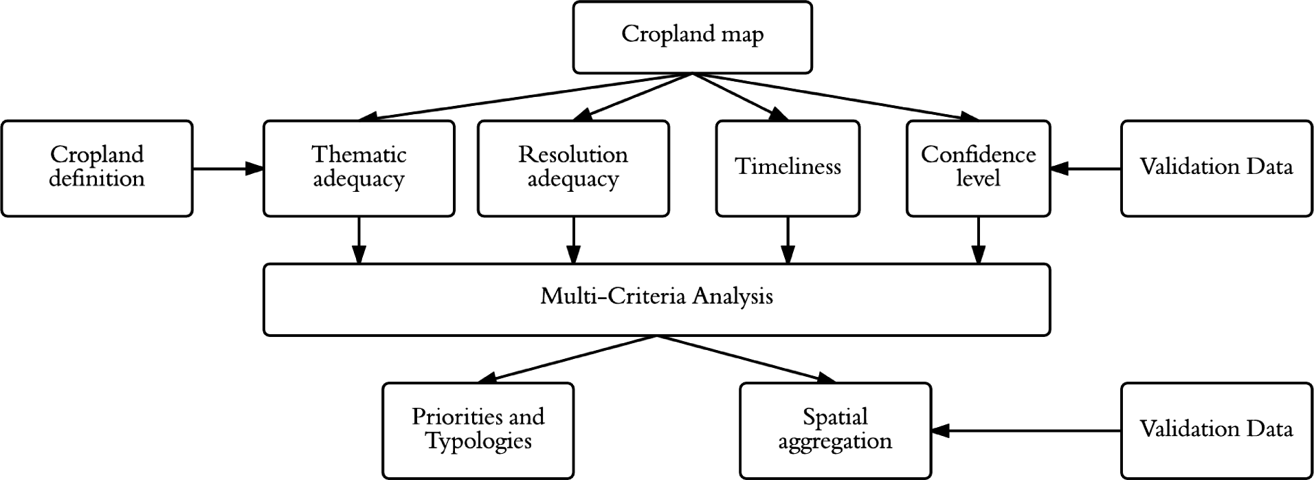
3. Method
- Constructing a database containing all of the spatial information;
- Transforming the chosen criteria into scores;
- Determining the weight for each criterion;
- Aggregating the data weights, obtaining the scores for each dataset and selecting the best score in overlapping regions.
3.1. Thematic Consistency Criterion
- Absence of woody crops (WC);
- Presence of fallow and bare fields (FB);
- Absence of managed pasture and meadows (MPM);
3.2. Timeliness Criterion
3.3. Resolution Adequacy Criterion
3.4. Confidence Level Criterion
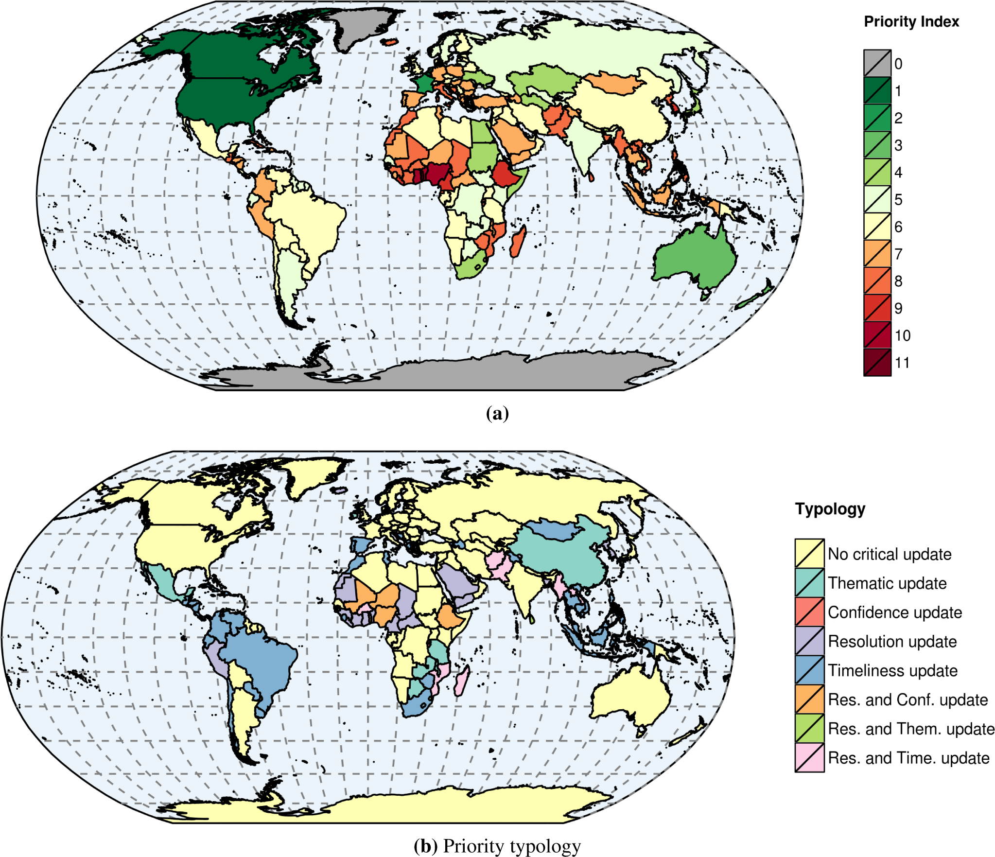
3.5. Criteria Aggregation and Priority Identification
3.6. Spatial Aggregation and Assessment
4. Results and Discussion
4.1. Multi-Criteria Analysis
4.2. Spatial Aggregation: Assessment and Comparison
5. Discussion
6. Conclusion
Acknowledgments
Author Contributions
Conflicts of Interest
References
- Fritz, S.; McCallum, I.; Schill, C.; Perger, C.; See, L.; Schepaschenko, D.; van der Velde, M.; Kraxner, F.; Obersteiner, M. Geo-Wiki: An online platform for improving global land cover. Environ. Model. Softw. 2012, 31, 110–123. [Google Scholar]
- Justice, C.O.; Becker-Reshef, I. Report from the Workshop on Developing a Strategy for Global Agricultural Monitoring in the Framework of Group on Earth Observations (GEO). Avaliable online: http://www.fao.org/gtos/igol/docs/meeting-reports/07-geo-ag0703-workshop-report-nov07.pdf accessed on 11 June 2015.
- Hannerz, F.; Lotsch, A. Assessment of remotely sensed and statistical inventories of African agricultural fields. Int. J. Remote Sens. 2008, 29, 3787–3804. [Google Scholar]
- Vancutsem, C.; Marinho, E.; Kayitakire, F.; See, L.; Fritz, S. Harmonizing and combining existing land cover/land use datasets for cropland area monitoring at the African continental scale. Remote Sens. 2012, 5, 19–41. [Google Scholar]
- Lobell, D.; Bala, G.; Duffy, P. Biogeophysical impacts of cropland management changes on climate. Geophys. Res. Lett. 2006, 33. [Google Scholar] [CrossRef]
- Yu, L.; Wang, J.; Clinton, N.; Xin, Q.; Zhong, L.; Chen, Y.; Gong, P. FROM-GC: 30 m global cropland extent derived through multisource data integration. Int. J. Digit. Earth. 2013, 6, 521–533. [Google Scholar]
- Bartholomé, E.; Belward, A. GLC2000: A new approach to global land cover mapping from Earth observation data. Int. J. Remote Sens. 2005, 26, 1959–1977. [Google Scholar]
- Arino, O.; Bicheron, P.; Achard, F.; Latham, J.; Witt, R.; Weber, J.L. The most detailed portrait of Earth. ESA Bull. 2008, 136, 25–31. [Google Scholar]
- Friedl, M.A.; McIver, D.K.; Hodges, J.C.; Zhang, X.; Muchoney, D.; Strahler, A.H.; Woodcock, C.E.; Gopal, S.; Schneider, A.; Cooper, A.; et al. Global land cover mapping from MODIS: Algorithms and early results. Remote Sens. Environ. 2002, 83, 287–302. [Google Scholar]
- Defourny, P.; Kirches, G.; Brockmann, C.; Boettcher, M.; Peters, M.; Bontemps, S.; Lamarche, C.; Schlerf, M.; Santoro, M. Land Cover CCI: Product User Guide Version 2. Available online: http://maps.elie.ucl.ac.be/CCI/viewer/download/ESACCI-LC-PUG-v2.4.pdf accessed on 11 June 2015.
- Gong, P.; Wang, J.; Yu, L.; Zhao, Y.; Zhao, Y.; Liang, L.; Niu, Z.; Huang, X.; Fu, H.; Liu, S.; et al. Finer resolution observation and monitoring of global land cover: First mapping results with Landsat TM and ETM+ data. Int. J. Remote Sens. 2013, 34, 2607–2654. [Google Scholar]
- Fritz, S.; See, L.; McCallum, I.; Schill, C.; Obersteiner, M.; van der Velde, M.; Boettcher, H.; Havlík, P.; Achard, F. Highlighting continued uncertainty in global land cover maps for the user community. Environ. Res. Lett. 2011, 6. [Google Scholar] [CrossRef]
- Ramankutty, N.; Evan, A.T.; Monfreda, C.; Foley, J.A. Farming the planet: 1. Geographic distribution of global agricultural lands in the year 2000. Glob. Biogeochem. Cycles 2008, 22. [Google Scholar] [CrossRef]
- Pittman, K.; Hansen, M.C.; Becker-Reshef, I.; Potapov, P.V.; Justice, C.O. Estimating global cropland extent with multi-year MODIS data. Remote Sens. 2010, 2, 1844–1863. [Google Scholar]
- Biradar, C.M.; Thenkabail, P.S.; Noojipady, P.; Li, Y.; Dheeravath, V.; Turral, H.; Velpuri, M.; Gumma, M.K.; Gangalakunta, O.R.P.; Cai, X.L.; et al. A global map of rainfed cropland areas (GMRCA) at the end of last millennium using remote sensing. Int. J. Appl. Earth Obs. Geoinf. 2009, 11, 114–129. [Google Scholar]
- Thenkabail, P.S.; Biradar, C.M.; Noojipady, P.; Dheeravath, V.; Li, Y.; Velpuri, M.; Gumma, M.; Gangalakunta, O.R.P.; Turral, H.; Cai, X.; et al. Global irrigated area map (GIAM), derived from remote sensing, for the end of the last millennium. Int. J. Remote Sens. 2009, 30, 3679–3733. [Google Scholar]
- Boryan, C.; Yang, Z.; Mueller, R.; Craig, M. Monitoring US agriculture: the US department of agriculture, national agricultural statistics service, cropland data layer program. Geocarto Int. 2011, 26, 341–358. [Google Scholar]
- Herold, M.; Woodcock, C.E.; Di Gregorio, A.; Mayaux, P.; Belward, A.S.; Latham, J.; Schmullius, C.C. A joint initiative for harmonization and validation of land cover datasets. IEEE Trans. Geosci. Remote Sens. 2006, 44, 1719–1727. [Google Scholar]
- Giri, C.; Zhu, Z.; Reed, B. A comparative analysis of the Global Land Cover 2000 and MODIS land cover data sets. Remote Sens. Environ. 2005, 94, 123–132. [Google Scholar]
- Foody, G.M. Status of land cover classification accuracy assessment. Remote Sens. Environ. 2002, 80, 185–201. [Google Scholar]
- Fritz, S.; See, L.; McCallum, I.; You, L.; Bun, A.; Moltchanova, E.; Duerauer, M.; Albrecht, F.; Schill, C.; Perger, C.; et al. Mapping global cropland and field size. Glob. Chang. Biol. 2015, 21, 1980–1992. [Google Scholar] [Green Version]
- Latham, J.; Cumani, R.; Rosati, I.; Bloise, M. Global Land Cover SHARE (GLC-SHARE) Database Beta-Release Version 1.0-2014. Available online: http://www.fao.org/uploads/media/glc-share-doc.pdf accessed on 11 June 2015.
- Xu, G.; Zhang, H.; Chen, B.; Zhang, H.; Yan, J.; Chen, J.; Che, M.; Lin, X.; Dou, X. A Bayesian based method to generate a synergetic land-cover map from existing land-cover products. Remote Sens. 2014, 6, 5589–5613. [Google Scholar]
- Herold, M.; Mayaux, P.; Woodcock, C.; Baccini, A.; Schmullius, C. Some challenges in global land cover mapping: An assessment of agreement and accuracy in existing 1 km datasets. Remote Sens. Environ. 2008, 112, 2538–2556. [Google Scholar]
- Eidenshink, J.C.; Faundeen, J.L. The 1 km AVHRR global land data set: First stages in implementation. Int. J. Remote Sens. 1994, 15, 3443–3462. [Google Scholar]
- Tateishi, R.; Hoan, N.T.; Kobayashi, T.; Alsaaideh, B.; Tana, G.; Phong, D.X. Production of Global Land Cover Data-GLCNMO2008. J. Geogr. Geol. 2014, 6, 99–122. [Google Scholar]
- Blanco, P.D.; Colditz, R.R.; Saldaña, G.L.; Hardtke, L.A.; Llamas, R.M.; Mari, N.A.; Fischer, A.; Caride, C.; Aceñolaza, P.G.; Del Valle, H.F.; et al. A land cover map of Latin America and the Caribbean in the framework of the SERENA project. Remote Sens. Environ. 2013, 132, 13–31. [Google Scholar]
- Verhegghen, A.; Mayaux, P.; de Wasseige, C.; Defourny, P. Mapping Congo Basin vegetation types from 300 m and 1 km multi-sensor time series for carbon stocks and forest areas estimation. Biogeosciences 2012, 9, 5061–5079. [Google Scholar] [Green Version]
- Miettinen, J.; Shi, C.; Tan, W.J.; Liew, S.C. land cover map of insular Southeast Asia in 250-m spatial resolution. Remote Sens. Lett. 3, 11–20.
- Klein, I.; Gessner, U.; Kuenzer, C. Regional land cover mapping and change detection in central Asia using MODIS time-series. Appl. Geogr. 2012, 35, 219–234. [Google Scholar]
- Chen, J.; Chen, J.; Liao, A.; Cao, X.; Chen, L.; Chen, X.; He, C.; Han, G.; Peng, S.; Lu, M.; et al. Global land cover mapping at 30 m resolution: A POK-based operational approach. ISPRS J. Photogramm. Remote Sens. 2015, 103, 7–27. [Google Scholar]
- Takahashi, M.; Nasahara, K.N.; Tadono, T.; Watanabe, T.; Dotsu, M.; Sugimura, T.; Tomiyama, N. JAXA high resolution land-use and land-cover map of Japan. Proceedings of 2013 IEEE International Geoscience and Remote Sensing Symposium (IGARSS), Melbourne, VIC, Australia, 21–26 July 2013; pp. 2384–2387.
- Thenkabail, P.S.; Wu, Z. An automated cropland classification algorithm (ACCA) for Tajikistan by combining Landsat, MODIS, and secondary data. Remote Sens. 2012, 4, 2890–2918. [Google Scholar]
- Liu, J.; Liu, M.; Tian, H.; Zhuang, D.; Zhang, Z.; Zhang, W.; Tang, X.; Deng, X. Spatial and temporal patterns of China’s cropland during 1990–2000: An analysis based on Landsat TM data. Remote Sens. Environ. 2005, 98, 442–456. [Google Scholar]
- Lymburner, L.; Tan, P.; Mueller, N.; Thackway, R.; Thankappan, M.; Islam, A.; Lewis, A.; Randall, L.; Senarath, U. The National Dynamic Land Cover Dataset; Geoscience Australia: Canberra, NSW, Astralia, 2011. [Google Scholar]
- Sreenivas, K.; Sekhar, N.S.; Saxena, M.; Paliwal, R.; Pathak, S.; Porwal, M.; Fyzee, M.; Rao, S.K.; Wadodkar, M.; Anasuya, T.; et al. Estimating inter-annual diversity of seasonal agricultural area using multi-temporal resourcesat data. J. Environ. Manag. 2014. [Google Scholar] [CrossRef]
- Holecz, F.; Collivignarelli, F.; Barbieri, M.; Gatti, L.; Boschetti, M.; Manfron, G.; Brivio, P.A.; Abukari, M.; Bondo, T. Establishing National Baseline Land Cover Map Including Annual and Seasonal Variations for the Understanding of Current Agricultural Practices in the Gambia; National Agricultural Land and Water Management Development Project (Nema), 2013; unpublished. [Google Scholar]
- Lavreniuk, M.; Kussul, N.; S., S.; Shelestov, A.; Yailymov, B. Regional retrospective high resolution land cover for Ukraine: Methodology and results. Proceedings of IEEE International Geoscience and Remote Sensing Symposium (IGARSS 2015), Milan, Italy, 26–31 July 2015. submitted.
- Bartalev, S.; Egorov, V.; Loupian, E.; Plotnikov, D.; Uvarov, I. Recognition of arable lands using multi-annual satellite data from spectroradiometer MODIS and locally adaptive supervised classification. Comput. Opt. 2011, 35, 103–116, In Russian. [Google Scholar]
- Defourny, P.; Schouten, L.; Bartalev, S.; Bontemps, S.; Cacetta, P.; Gérard, B.; Giri, C.; Gond, V.; Hazeu, G.; Heinimann, A.; et al. Accuracy assessment of a 300 m global land cover map: The GlobCover experience. Proceedings of the 33rd International Symposium on Remote Sensing of Environment, Stresa, Italy, 4–8 May 2009.
- Defourny, P.; Mayaux, P.; Herold, M.; Bontemps, S. Global land-cover map validation experiences: Toward the characterization of quantitative uncertainty. In Remote Sensing of Land Use and Land Cover: Principles and Applications; Giri, C.P., Ed.; CRC Press: London, UK, 2012; pp. 207–223. [Google Scholar]
- Olofsson, P.; Stehman, S.V.; Woodcock, C.E.; Sulla-Menashe, D.; Sibley, A.M.; Newell, J.D.; Friedl, M.A.; Herold, M. A global land-cover validation data set, part I: Fundamental design principles. Int. J. Remote Sens. 2012, 33, 5768–5788. [Google Scholar]
- Stehman, S.V.; Olofsson, P.; Woodcock, C.E.; Herold, M.; Friedl, M.A. A global land-cover validation data set, II: Augmenting a stratified sampling design to estimate accuracy by region and land-cover class. Int. J. Remote Sens. 2012, 33, 6975–6993. [Google Scholar]
- GOFC-GOLD. STEP Reference Dataset. 2011. Available online: http://www.gofcgold.wur.nl/sites/gofcgold_refdataportal-step.php accessed on 11 June 2015.
- Zhao, Y.; Gong, P.; Yu, L.; Hu, L.; Li, X.; Li, C.; Zhang, H.; Zheng, Y.; Wang, J.; Zhao, Y.; et al. Towards a common validation sample set for global land-cover mapping. Int. J. Remote Sens. 2014, 35, 4795–4814. [Google Scholar]
- Fritz, S.; McCallum, I.; Schill, C.; Perger, C.; Grillmayer, R.; Achard, F.; Kraxner, F.; Obersteiner, M. Geo-Wiki. org: The use of crowdsourcing to improve global land cover. Remote Sens. 2009, 1, 345–354. [Google Scholar]
- Setegn, S.G.; Srinivasan, R.; Dargahi, B.; Melesse, A.M. Spatial delineation of soil erosion vulnerability in the Lake Tana Basin, Ethiopia. Hydrol. Process. 2009, 23, 3738–3750. [Google Scholar]
- Mourão, K.R.M.; Sousa Filho, P.W.M.; de Oliveira Alves, P.J.; Frédou, F.L. Priority areas for the conservation of the fish fauna of the Amazon Estuary in Brazil: A multicriteria approach. Ocean Coastal Manag. 2014, 100, 116–127. [Google Scholar]
- Iojă, C.I.; Ni¸tă, M.R.; Vânău, G.O.; Onose, D.A.; Gavrilidis, A.A. Using multi-criteria analysis for the identification of spatial land-use conflicts in the Bucharest Metropolitan Area. Ecol. Indic. 2014, 42, 112–121. [Google Scholar]
- McCallum, I.; Obersteiner, M.; Nilsson, S.; Shvidenko, A. A spatial comparison of four satellite derived 1km global land cover datasets. Int. J. Appl. Earth Obs. Geoinf. 2006, 8, 246–255. [Google Scholar]
- Di Gregorio, A.; Jansen, L.J. Land Cover Classification System (LCCS): Classification Concepts and User Manual, version 1.0; Food and Agriculture Organization of the United Nations: Rome, Italy, 2000. [Google Scholar]
- del Mar López, T.; Aide, T.M.; Thomlinson, J.R. Urban expansion and the loss of prime agricultural lands in Puerto Rico. Ambio 2001, 30, 49–54. [Google Scholar]
- Morton, D.C.; DeFries, R.S.; Shimabukuro, Y.E.; Anderson, L.O.; Arai, E.; del Bon Espirito-Santo, F.; Freitas, R.; Morisette, J. Cropland expansion changes deforestation dynamics in the southern Brazilian Amazon. Proc. Natl. Acad. Sci. USA 2006, 103, 14637–14641. [Google Scholar]
- Benayas, J.R.; Martins, A.; Nicolau, J.M.; Schulz, J.J. Abandonment of agricultural land: an overview of drivers and consequences. CAB Rev. Perspect. Agric. Vet. Sci. Nutr. Nat. Resour. 2007, 2, 1–14. [Google Scholar]
- Baumann, M.; Kuemmerle, T.; Elbakidze, M.; Ozdogan, M.; Radeloff, V.C.; Keuler, N.S.; Prishchepov, A.V.; Kruhlov, I.; Hostert, P. Patterns and drivers of post-socialist farmland abandonment in western Ukraine. Land Use Policy 2011, 28, 552–562. [Google Scholar]
- Löw, F.; Duveiller, G. Defining the spatial resolution requirements for crop identification using optical remote sensing. Remote Sens. 2014, 6, 9034–9063. [Google Scholar]
- Leroux, L.; Jolivot, A.; Bégué, A.; Seen, D.L.; Zoungrana, B. How reliable is the MODIS land cover product for crop mapping sub-saharan agricultural landscapes? Remote Sens. 2014, 6, 8541–8564. [Google Scholar]
- Vintrou, E.; Desbrosse, A.; Bégué, A.; Traoré, S.; Baron, C.; Seen, D.L. Crop area mapping in West Africa using landscape stratification of MODIS time series and comparison with existing global land products. Int. J. Appl. Earth Obs. Geoinf. 2012, 14, 83–93. [Google Scholar]
- Saaty, T.L. How to make a decision: The analytic hierarchy process. Eur. J. Oper. Res. 1990, 48, 9–26. [Google Scholar]
- Mendoza, G.; Prabhu, R. Multiple criteria analysis for assessing criteria and indicators in sustainable forest management: A case study on participatory decision making in a Kalimantan forest. Environ. Manag. 2000, 26, 659–673. [Google Scholar]
- Hansen, M.C.; Potapov, P.V.; Moore, R.; Hancher, M.; Turubanova, S.; Tyukavina, A.; Thau, D.; Stehman, S.; Goetz, S.; Loveland, T.; et al. High-resolution global maps of 21st-century forest cover change. Science 2013, 342, 850–853. [Google Scholar]
- Shimada, M.; Itoh, T.; Motooka, T.; Watanabe, M.; Shiraishi, T.; Thapa, R.; Lucas, R. New global forest/non-forest maps from ALOS PALSAR data 2007–2010. Remote Sens. Environ. 2014, 155, 13–31. [Google Scholar]
- Tsendbazar, N.; de Bruin, S.; Herold, M. Assessing global land cover reference datasets for different user communities. ISPRS J. Photogramm. Remote Sens. 2015, 103, 93–114. [Google Scholar]
- Goldewijk, K.K.; van Drecht, G.; Bouwman, A.F. Mapping contemporary global cropland and grassland distributions on a 5 × 5 minute resolution. J. Land Use Sci. 2007, 2, 167–190. [Google Scholar]
- See, L.; Fritz, S.; You, L.; Ramankutty, N.; Herrero, M.; Justice, C.; Becker-Reshef, I.; Thornton, P.; Erb, K.; Gong, P.; et al. Improved global cropland data as an essential ingredient for food security. Glob. Food Secur. 2014, 4, 37–45. [Google Scholar]
- Whitcraft, A.K.; Vermote, E.F.; Becker-Reshef, I.; Justice, C.O. Cloud cover throughout the agricultural growing season: Impacts on passive optical earth observations. Remote Sens. Environ. 2015, 156, 438–447. [Google Scholar]
- Blaes, X.; Vanhalle, L.; Defourny, P. Efficiency of crop identification based on optical and SAR image time series. Remote Sens. Environ. 2005, 96, 352–365. [Google Scholar]
- McNairn, H.; Shang, J.; Champagne, C.; Jiao, X. TerraSAR-X and RADARSAT-2 for crop classification and acreage estimation. Proceedings of 2009 IEEE International Geoscience and Remote Sensing Symposium, Cape Town, South Africa, 12–17 July 2009; 2, pp. II-898–II-901.
- McNairn, H.; Champagne, C.; Shang, J.; Holmstrom, D.; Reichert, G. Integration of optical and Synthetic Aperture Radar (SAR) imagery for delivering operational annual crop inventories. ISPRS J. Photogramm. Remote Sens. 2009, 64, 434–449. [Google Scholar]
- McNairn, H.; Kross, A.; Lapen, D.; Caves, R.; Shang, J. Early season monitoring of corn and soybeans with TerraSAR-X and RADARSAT-2. Int. J. Appl. Earth Obs. Geoinf. 2014, 28, 252–259. [Google Scholar]
- Jia, K.; Li, Q.; Tian, Y.; Wu, B.; Zhang, F.; Meng, J. Crop classification using multi-configuration SAR data in the North China Plain. Int. J. Remote Sens. 2012, 33, 170–183. [Google Scholar]
- Forkuor, G.; Conrad, C.; Thiel, M.; Ullmann, T.; Zoungrana, E. Integration of optical and Synthetic Aperture Radar imagery for improving crop mapping in northwestern Benin, West Africa. Remote Sens. 2014, 6, 6472–6499. [Google Scholar]
- Kussul, N.; Skakun, S.; Kravchenko, O.; Shelestov, A.; Gallego, J.F.; Kussul, O. Application of satellite optical and SAR images for crop mapping and erea estimation in Ukraine. Int. J. Inf. Model. Anal. 2013, 7, 203–211. [Google Scholar]
- Gao, F.; Masek, J.; Schwaller, M.; Hall, F. On the blending of the Landsat and MODIS surface reflectance: Predicting daily Landsat surface reflectance. IEEE Trans. Geosci. Remote Sens. 2006, 44, 2207–2218. [Google Scholar]
- Bisquert, M.; Bordogna, G.; Bégué, A.; Candiani, G.; Teisseire, M.; Poncelet, P. A simple fusion method for image time series based on the estimation of image temporal validity. Remote Sens. 2015, 7, 704–724. [Google Scholar]


| Extent | Product Name and Reference | Epoch |
|---|---|---|
| Global | FROM-GLC [11] | 2013 |
| Global Cropland Extent [14] | 2000–2008 | |
| GlobCover 2009 [8] | 2009 | |
| Climate Change Initiative Land Cover (CCI) [10] | 2008–2012 | |
| MOD12Q1, NASA | 2005 | |
| GLC-Share, Food and Agriculture Organization [22] | 1990–2012 | |
| IIASA-IFPRICropland [21] | 1990–2012 | |
| GLC2000 [7] | 1999–2000 | |
| International Geosphere-Biosphere Programme (IGBP) [25] | 1992–1993 | |
| Global Map-Global Land Cover (GLCNMO) [26] | 2007–2009 | |
| Regional | Corine Land Cover, European Environment Agency (EEA) | 2006 |
| Southern African Development Community Land Cover database, Council for Scientific and Industrial Research (CSIR) | 2002 | |
| Cropland Mask of Africa, Joint Research Centre (JRC) [4] | 2012 | |
| North American Environmental Atlas, Commission for Environmental Cooperation (CEC) | 2005 | |
| Land Cover Map of Latin America and the Caribbean [27] | 2008 | |
| Congo Basin Map [28] | 2000–2007 | |
| Land cover map of insular Southeast Asia [29] | 2010 | |
| Land Cover Central Asia [30] | 2009 | |
| Congo, Burundi, Egypt, Eritrea, Kenya, Rwanda, Somalia, Sudan, Tanzania, Uganda | Africover, Food and Agriculture Organization (FAO) | 1999–2001 |
| Senegal, Bhutan, Nepal | Global Land Cover Network (GLCN) | 2005–2007 |
| France, Belgium, the Netherlands | Land Parcel Identification System | 2012–2014 |
| Barbados, Rep. Dominicana, Dominica, Grenada, Puerto Rico, Saint Kit and Nevis, Virgin Islands | United States Geological Survey (USGS) | 2000–2001 |
| Fiji, Solomon Islands, Timor Leste, Niue, Naurau, Palau, Tonga, Tuvalu, Vanuatu, Kiribati, Marshall Islands, Micronesia, Cook Islands | Applied Geoscience and Technology Division (SOPAC) | 1999–2010 |
| Botswana, Namibia, Rwanda, Zambia, Tanzania, Malawi | Land Cover Scheme II, the Regional Visualization and Monitoring System (ICIMOD-SERVIR) | 2010 |
| China | GlobeLand30 [31] | 2009–2011 |
| Japan | High Resolution Land Use-Land Cover Map, Japan Aerospace Exploration Agency (JAXA) [32] | 2006–2011 |
| Tajikistan | [33] | 2010 |
| Burkina Faso | Corine Database of Burkina Faso | 2000 |
| Canada | Annual Crop Inventory, Agri-Food Canada (AAFC) | 2013 |
| USA | Cropland Data Layer, US Department of Agriculture (USDA) | 2013 |
| China | National Land Cover Map of China [34] | 1995–1996 |
| Australia | Digital Land Cover Database [35] | 2011 |
| Cambodia | Land Cover of Cambodia, Japan International Cooperation Agency (JICA) | 2002 |
| New Zealand | Land Cover DataBase v4 Ministry for the Environment | 2004 |
| South Africa | National Land Cover, CSIR | 2000–2001 |
| South Africa | National Land Cover, South African National Biodiversity Institute (SANBI) | 2009 |
| Canada | National Resources of Canada | 2005 |
| Uruguay | Land Cover of Uruguay, FAO | 2010 |
| Mexico | Land Cover of Mexico,Comisión Nacional para el Conocimiento y Uso de la Biodiversidad (CONABIO) | 1999 |
| Argentina | Cobertura y uso del suelo, Instituto Nacional de Tecnología Agropecuaria (INTA) | 2006 |
| Ecuador | Uso del Suelo departamento de Informacíon Ambiental | 2001 |
| Thailand | Royal Forest Department of Thailand | 2000 |
| Chile | Chile Corporacion Nacional Forestal | 1999 |
| India | Land Use Land Cover of India, National Remote Sensing Centre (NRSC) [36] | 2012 |
| Gambia | [37] | 2013 |
| Ukraine | Land Cover Ukraine [38] | 2010 |
| Russia | TerraNorte Arable Lands of Russia [39] | 2014 |
| Validation Set | Geometry | Sample Size | Cropland (%) |
|---|---|---|---|
| GlobCover 2005 | Polygon (225 ha) | 186 | 9 |
| VIIRS | Polygon (5 × 5 km) | 3664 | 27 |
| STEP | Polygon (4 × 4-km) | 1780 | 26 |
| GLC-2000 | Point | 1253 | 9 |
| Zhao et al. | Point | 38,664 | 7 |
| GeoWiki | Polygon (1 × 1-km) | 12,833 | 29 |
| (a) Rules for the Thematic Criterion
| ||
|---|---|---|
| Thematic Criterion | Code | Score |
| 3 | Good thematic agreement | 4 |
| 2 | Moderate thematic agreement | 3 |
| 1 | Low thematic agreement | 2 |
| 0 | No thematic agreement | 1 |
| (b) Rules for the Timeliness Criterion
| ||
|---|---|---|
| Timeliness Criterion | Code | Score |
| 1–2 | Up-to-date | 4 |
| 2–5 | Recent | 3 |
| 5–10 | Old | 2 |
| 10> | Out-of-date | 1 |
| (c) Rules for the Resolution Adequacy Criterion
| ||
|---|---|---|
| Resolution Adequacy Criterion | Code | Score |
| >0 | Completely adequate | 4 |
| 1 | Adequate | 3 |
| 2 | Inadequate | 2 |
| 3 | Completely Inadequate | 1 |
| (d) Rules for the Confidence Level Criterion
| ||
|---|---|---|
| Confidence Level Criterion | Code | Score |
| 80%–100% | High confidence level | 4 |
| 70%–80% | Good confidence level | 3 |
| 60%–70% | Low confidence | 2 |
| 0%–60% | Very low confidence level | 1 |
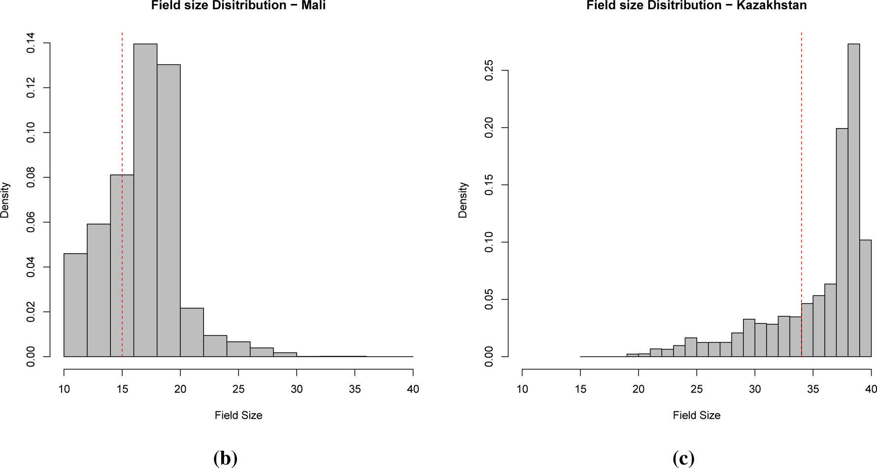
| GeoWiki Field Size | GEOGLAM Field Size (ha) | GEOGLAM Resolution Requirements (m) |
|---|---|---|
| Large | >15 | 100–500 |
| Medium | >1.5 | 20–100 |
| Small | >0.15 | 5–20 |
| Very Small | <0.15 | <5 |
| (a)Confusion Matrix Obtained with the GlobCover 2005 Dataset
| |||
|---|---|---|---|
| Non-Cropland | Cropland | User’s Accuracy (%) | |
| Non-Cropland | 158 | 9 | 95.2 |
| Cropland | 2 | 16 | 87.5 |
| Producer’s Accuracy (%) | 98.8 | 63.6 | Overall Accuracy (%): 94.5 |
| (b) Confusion Matrix Obtained with the VIIRS Dataset
| |||
|---|---|---|---|
| Non-Cropland | Cropland | User’s Accuracy (%) | |
| Non-Cropland | 631 | 63 | 89.4 |
| Cropland | 251 | 985 | 87.5 |
| Producer’s Accuracy (%) | 85.9 | 72.2 | Overall Accuracy (%): 82.3 |
| (c) Confusion Matrix Obtained with the GeoWiki Dataset
| |||
|---|---|---|---|
| Non-Cropland | Cropland | User’s Accuracy (%) | |
| Non-Cropland | 8490 | 384 | 95.6 |
| Cropland | 1698 | 2055 | 54.7 |
| Producer’s Accuracy (%) | 83.3 | 84.3 | Overall Accuracy (%): 82.2 |
| (d) Confusion Matrix Obtained for the Unified Cropland Layer Masked by the ALOS PALSAR Forest Mask with the GeoWiki Dataset
| |||
|---|---|---|---|
| Non-Cropland | Cropland | User’s Accuracy (%) | |
| Non-Cropland | 8085 | 999 | 89.0 |
| Cropland | 986 | 2763 | 73.7 |
| Producer’s Accuracy (%) | 89.1 | 73.4 | Overall Accuracy (%): 84.5 |
© 2015 by the authors; licensee MDPI, Basel, Switzerland This article is an open access article distributed under the terms and conditions of the Creative Commons Attribution license (http://creativecommons.org/licenses/by/4.0/).
Share and Cite
Waldner, F.; Fritz, S.; Di Gregorio, A.; Defourny, P. Mapping Priorities to Focus Cropland Mapping Activities: Fitness Assessment of Existing Global, Regional and National Cropland Maps. Remote Sens. 2015, 7, 7959-7986. https://doi.org/10.3390/rs70607959
Waldner F, Fritz S, Di Gregorio A, Defourny P. Mapping Priorities to Focus Cropland Mapping Activities: Fitness Assessment of Existing Global, Regional and National Cropland Maps. Remote Sensing. 2015; 7(6):7959-7986. https://doi.org/10.3390/rs70607959
Chicago/Turabian StyleWaldner, François, Steffen Fritz, Antonio Di Gregorio, and Pierre Defourny. 2015. "Mapping Priorities to Focus Cropland Mapping Activities: Fitness Assessment of Existing Global, Regional and National Cropland Maps" Remote Sensing 7, no. 6: 7959-7986. https://doi.org/10.3390/rs70607959