Backscatter Analysis Using Multi-Temporal and Multi-Frequency SAR Data in the Context of Flood Mapping at River Saale, Germany

Abstract

In this study, an analysis of multi-temporal and multi-frequency Synthetic Aperture Radar data is performed to investigate the backscatter behavior of various semantic classes in the context of flood mapping in central Europe. The focus is mainly on partially submerged vegetation such as forests and agricultural fields. The test area is located at River Saale, Saxony-Anhalt, Germany, which is covered by a time series of 39 TerraSAR-X data acquired within the time interval December 2009 to June 2013. The data set is supplemented by ALOS PALSAR L-band and RADARSAT-2 C-band data. The time series covers two inundations in January 2011 and June 2013 which allows evaluating backscatter variations between flood periods and normal water level conditions using different radar wavelengths. According to the results, there is potential in detecting flooding beneath vegetation in all microwave wavelengths, even in X-band for sparse vegetation or leaf-off forests.

1. Introduction

Synthetic Aperture Radar (SAR) is the preferred tool for flood mapping from space. This is due to the following reasons: On the one hand, a SAR sensor provides its own source of illumination in the microwave range. Therefore, it is characterized by near all-weather/day-night imaging capabilities independent of atmospheric conditions. This guarantees a continuous observation of the earth. On the other hand, smooth open water areas can be easily detected in the radar data. A flat water surface acts as a specular reflector which scatters the radar energy away from the sensor. This causes relatively dark pixels in radar data which contrast with non-water areas. Further, in comparison to optical sensors, SAR offers the unique opportunity to detect—to a certain extent—standing water beneath vegetation. The detectability of partially submerged vegetation is enabled by multiple-bounce effects: The penetrated radar signal is backscattered from the horizontal water surface and lower sections of the vegetation (e.g., branches and trunks). Compared to normal water level conditions, this leads to an increased backscatter return to the sensor [1,2], as diffuse scattering on the ground reduces the corner reflection effect.

Since the launch of the high resolution SAR satellite systems TerraSAR-X, RADARSAT-2 and the COSMO-SkyMed constellation, a limited number of automatic image processing algorithms has been developed to derive open flood surfaces from SAR data [3,4,5,6,7]. Only few fully operational SAR-based flood mapping services have been presented in the literature so far based on TerraSAR-X [4] and Envisat ASAR [8,9] data. Automatic flood mapping algorithms generally only focus on open water areas and do not consider partially submerged vegetation areas. This is due to the fact that the signal return from partially flooded vegetation is very complex and strongly depends on SAR system parameters (particularly wavelength, polarization and incidence angle) and environmental parameters (canopy type, structure and density) [10,11,12,13].

In general, the longer the system’s wavelength, the higher is the capability of the signal to penetrate the vegetation canopy. Several studies present the potential of L-band [1,14,15,16,17] and C-band SAR [2,13,16,18,19] data for detecting inundations beneath forests. Using X-band SAR, canopy attenuation, volume and surface scattering from the top layer of the forest canopy is generally higher [1]. This reduces the effect of double bounce scattering, which is related to a decreased ratio between the backscatter of non-flooded and flooded forests. With decreasing wavelength double bounce scattering may also occur at shorter or sparser vegetation with thin branches and small diameter trunks. Therefore, some studies indicate a certain potential to detect flooded vegetation using X-band SAR data, e.g., over leaf-off forests [20]) and marshland environments [18,21], olive groves [22] as well as grassland and foliated shrubs [23,24]. However, there exist several objects which may have similar backscatter values as double bouncing vegetation and could result in an overestimation of the flood extent such as double bounce effects in urban areas, layover effects on vertical object (e.g., mountains, urban structures), anthropogenic features on the water surface (e.g., ships, debris), roughened water surfaces as well as soils with high moisture conditions. Also, the backscatter over partially flooded crop land, which is characterized by rigid plant structures and sparse leaf coverage, in most cases increases due to double bounce effects [25]. Even though there exist extensive studies in monitoring rice crops (see Mosleh et al. [26] for a review), the backscatter behavior of other flooded crop types in relation to pre-flood events are rarely described in detail in the literature, and the actual results of the corresponding backscatter changes are difficult to determine due to double-bounce effects.

Furthermore, the incidence angle has significant influence on the backscatter process from flooded vegetation areas. This has to be considered in classification algorithms, especially when the data are characterized by a large range of incidence angles between near and far range [19,27]. Several studies have shown that steep incidence angles are better suited than shallow ones for flood mapping in forests [1,10,13,28,29,30,]. This generalization can be related to a shorter path of the SAR signal through the canopy. As a consequence, the transmissivity of the crown layer increases and more microwave energy is available for ground-trunk interactions. In contrast, shallower incidence angle signals have a stronger interaction with the canopy. This results in increased volume scattering [13,28].

Radar systems with multiple polarizations provide more information on inundated vegetation areas than single-polarized SAR [16,21,31]. Studies employing multi-polarized data indicate advantages of like-polarization (HH or VV) for the seperation of flooded and non-flooded forests [11,32]. According to [12,30], the backscatter ratio between flooded and non-flooded forest is higher at HH polarization than at VV polarization. Backscatter is generally lower for cross-polarization (HV or VH) as depolarization does not make for ideal corner reflectors [33].

Table 1 gives an overview about the main findings in the literature concerning the mapping of double-bouncing flooded vegetation areas with a focus on backscatter variations between flooded and dry conditions and empirical threshold values used for separating flooded vegetation. Study areas are mainly situated in Northern America, South America, and Australia. Only two study areas are located in Europe (Estonia and Italy). Backscatter increases due to flooding occur in all SAR bands over vegetation areas. The following maximum backscatter differences between flooded and non-flooded conditions have been stated for different SAR wavelengths: X-band: 10 dB [22], C-band: 6.9 dB [20], and L-band: 9.7 dB [1]. The results are very heterogeneous and depend strongly on environmental and system parameters. Threshold values separating flooded and non-flooded regions are therefore hardly transferable to other test areas and have to be defined individually.

As the use of multiple-polarization data has significant advantages over single-polarized data in detecting water below vegetation canopies, mostly multi-polarized data are acquired in continuous wetland monitoring programs. In contrast, during flood rapid mapping activities, data are commonly acquired without a priori knowledge about the existence of flooded vegetation and it is assumed that most of the flood area consists of open water bodies. Therefore, single-polarized data (HH) are used to derive the flood extent in high spatial resolution. e.g., the use of TerraSAR-X scenes acquired in ScanSAR (pixel spacing: 8.25 m) or Wide ScanSAR (spatial resolution: ~40 m) mode allow the monitoring of large flood events—however, these modes are restricted to single polarization. Dual polarized acquisitions in Stripmap mode are related to a bisection of the swath width and a reduction of the spatial resolution. The derivation of flooded vegetation surfaces during operational flood rapid mapping activities is therefore in most cases restricted to single-polarized data.

Table 1. Overview about the main findings in the literature concerning the mapping of flooded vegetation areas.

Reference	Vegetation Type	Study Area	SAR System	Main Results
Engheta & Elachi [14]	Swamp with deciduous forest	Arkansas, USA	Seasat (L-band)	σ0 increase: Δ3–6 dB
Ormsby et al. [15]	Pine, ash, other deciduous	Maryland, USA	Seasat (L-band)	σ0 increase: Δ2.5–6.3 dB
Richards et al. [1]	Mono-specific eucalyptus forest	Murray River, Australia	SIR-B (L-band)	σ0 increase: Δ9.7 dB
Wang & Imhoff [29]	Mangrove forests: Sundri and Gewa trees	Ganges delta, Bangladesh	SIR-B (L-band)	σ0 increase in dependence of inc. angle [°]: Gewa: Δ3.4 (26°), Δ3.4 (48°) Gewa with Sundri: Δ1.6 (26°), Δ3.3 (48°) Sundri with Gewa: Δ3.8 (26°), Δ1.6 (48°)
Ramsey [18]	Coastal wetlands/black needlerush marsh	Florida, USA	ERS-1 (C-band)	Fluctuations in water level of 25 cm above to 7 cm below the marsh surface results in variations of SAR signal of −15.1 to −6.8 dB.
Rignot et al. [31]	Tropical moist rain forest	Rondonia, Brazil	JERS-1 (L-band), SIR-C (C-/L-band)	σ0 increase: Δ3.0 dB at LHH and Δ2.9 dB at CHH beetween primary forest and flooded dead forest (moist trunks and absence of live canopy)
Townsend [2]	Forested wetland	Roanoke River, North Carolina, USA	RADARSAT-1 (C-band)	Threshold of flooded leaf-off forest: −4.2 dB Threshold of flooded leaf-on forest: −5.1 dB and lower (at least 1 dB lower than over leaf-off forests) Threshold for flooded forest data with steep incidence angle: −4.21 dB Threshold for flooded forest data with shallow incidence angle: −8.21 dB → Difference of Δ4 dB between flooded forests imaged in S2 and S6 modes
Hess & Melack [16]	Woody and herbaceous vegetation	East Alligator River, North Australia	SIR-C (C-/L-band, HH and HV)	Backscatter in October (dry season) compared to April (wet season) : Maximum decrease from April to October in median σ0 (HH) for an individual stand: Δ5.8 dB at CHH and Δ6.4 dB at LHH Cross-polarized differences are smaller: Δ2.3 and Δ2.8 dB decreases at CHV and LHV.
Hess et al. [28]	Herbaceous, shrub, woodland, forest, palms	Central Amazon	JERS-1 (L-band)	Class median of non-flooded forest: −7.4 dB σ0 increase due to flooding: Δ2.1 dB Median σ0 for aquatic macrophytes (herbaceous-flooded): −8.3 dB Woodland-flooded (median σ0: −6.8 dB): largest dynamic range (~7 dB) separating the 5% (−11.5 dB) and 95% quantile (−4.6 dB) Shrub-non-flooded (median σ0: −8.8dB) with herbaceous-flooded Shrub-flooded (median σ0: −4.5 dB) with forest-/woodland-/palm-flooded A threshold of −6.5 dB separates flooded from non-flooded forest
Horritt et al. [21]	Emergent salt marsh	East coast UK	Airborne SAR (C-/L-band)	σ0 increase of ~Δ1.2 dB at C-band, and 180° HH-VV phase differences at L-band.
Martinez & Le Toan [17]	Alluvial forest	Amazon River, Brazil	JERS-1 (L-band)	σ0 increase of ca. Δ 2.0–Δ 3.0 dB during seasonal flooding
Lang et al. [13]	Forest (tupelo-cypress, bottomland hardwood)	Roanoke River, North Carolina, USA	RADARSAT-1 (C-band)	σ0 decrease with increasing incidence angle during floods (leaf-on period/incidence angles: 23.5°–43.5°: Δ0.62 dB; leaf-off period/incidence angles: 23.5°–47.0°: Δ2.45 dB
Pulvirenti et al. [22]	Olive groves, deciduous forest	Tuscany, Italy	COSMO-SkyMed (X-band)	σ0 increase of Δ7.0–8.6 dB (biomass: 50 t/ha) and Δ10 dB (biomass: 25 t/ha) Thresholds: Flooded areas: Δ > 7.0 dB Non-flooded areas: Δ < 3.0 dB
Voormansik et al. [20]	Coniferous, deciduous leaf-off forest	Estonia	TerraSAR-X (X-band), Envisat ASAR (C-Band)	Mixed forest: TerraSAR-X σ0 increase: Δ3.2 dB; Envisat ASAR: Δ6.9 dB Deciduous forest: TerraSAR-X σ0 increase: Δ6.2 dB; Envisat ASAR: Δ4.6 dB Coniferous forest: TerraSAR-X σ0 increase: Δ4.0 dB; Envisat ASAR: Δ6.4 dB
Martinis et al. [24]	Grassland and foliated shrubs	Caprivi, Namibia	TerraSAR-X (X-band)	σ0 over flooded vegetation −4 to −5 dB. σ0 difference to pre-flood conditions (Δ6.5–7.5 dB)

Table 1. Overview about the main findings in the literature concerning the mapping of flooded vegetation areas.

Reference	Vegetation Type	Study Area	SAR System	Main Results
Engheta & Elachi [14]	Swamp with deciduous forest	Arkansas, USA	Seasat (L-band)	σ0 increase: Δ3–6 dB
Ormsby et al. [15]	Pine, ash, other deciduous	Maryland, USA	Seasat (L-band)	σ0 increase: Δ2.5–6.3 dB
Richards et al. [1]	Mono-specific eucalyptus forest	Murray River, Australia	SIR-B (L-band)	σ0 increase: Δ9.7 dB
Wang & Imhoff [29]	Mangrove forests: Sundri and Gewa trees	Ganges delta, Bangladesh	SIR-B (L-band)	σ0 increase in dependence of inc. angle [°]: Gewa: Δ3.4 (26°), Δ3.4 (48°) Gewa with Sundri: Δ1.6 (26°), Δ3.3 (48°) Sundri with Gewa: Δ3.8 (26°), Δ1.6 (48°)
Ramsey [18]	Coastal wetlands/black needlerush marsh	Florida, USA	ERS-1 (C-band)	Fluctuations in water level of 25 cm above to 7 cm below the marsh surface results in variations of SAR signal of −15.1 to −6.8 dB.
Rignot et al. [31]	Tropical moist rain forest	Rondonia, Brazil	JERS-1 (L-band), SIR-C (C-/L-band)	σ0 increase: Δ3.0 dB at LHH and Δ2.9 dB at CHH beetween primary forest and flooded dead forest (moist trunks and absence of live canopy)
Townsend [2]	Forested wetland	Roanoke River, North Carolina, USA	RADARSAT-1 (C-band)	Threshold of flooded leaf-off forest: −4.2 dB Threshold of flooded leaf-on forest: −5.1 dB and lower (at least 1 dB lower than over leaf-off forests) Threshold for flooded forest data with steep incidence angle: −4.21 dB Threshold for flooded forest data with shallow incidence angle: −8.21 dB → Difference of Δ4 dB between flooded forests imaged in S2 and S6 modes
Hess & Melack [16]	Woody and herbaceous vegetation	East Alligator River, North Australia	SIR-C (C-/L-band, HH and HV)	Backscatter in October (dry season) compared to April (wet season) : Maximum decrease from April to October in median σ0 (HH) for an individual stand: Δ5.8 dB at CHH and Δ6.4 dB at LHH Cross-polarized differences are smaller: Δ2.3 and Δ2.8 dB decreases at CHV and LHV.
Hess et al. [28]	Herbaceous, shrub, woodland, forest, palms	Central Amazon	JERS-1 (L-band)	Class median of non-flooded forest: −7.4 dB σ0 increase due to flooding: Δ2.1 dB Median σ0 for aquatic macrophytes (herbaceous-flooded): −8.3 dB Woodland-flooded (median σ0: −6.8 dB): largest dynamic range (~7 dB) separating the 5% (−11.5 dB) and 95% quantile (−4.6 dB) Shrub-non-flooded (median σ0: −8.8dB) with herbaceous-flooded Shrub-flooded (median σ0: −4.5 dB) with forest-/woodland-/palm-flooded A threshold of −6.5 dB separates flooded from non-flooded forest
Horritt et al. [21]	Emergent salt marsh	East coast UK	Airborne SAR (C-/L-band)	σ0 increase of ~Δ1.2 dB at C-band, and 180° HH-VV phase differences at L-band.
Martinez & Le Toan [17]	Alluvial forest	Amazon River, Brazil	JERS-1 (L-band)	σ0 increase of ca. Δ 2.0–Δ 3.0 dB during seasonal flooding
Lang et al. [13]	Forest (tupelo-cypress, bottomland hardwood)	Roanoke River, North Carolina, USA	RADARSAT-1 (C-band)	σ0 decrease with increasing incidence angle during floods (leaf-on period/incidence angles: 23.5°–43.5°: Δ0.62 dB; leaf-off period/incidence angles: 23.5°–47.0°: Δ2.45 dB
Pulvirenti et al. [22]	Olive groves, deciduous forest	Tuscany, Italy	COSMO-SkyMed (X-band)	σ0 increase of Δ7.0–8.6 dB (biomass: 50 t/ha) and Δ10 dB (biomass: 25 t/ha) Thresholds: Flooded areas: Δ > 7.0 dB Non-flooded areas: Δ < 3.0 dB
Voormansik et al. [20]	Coniferous, deciduous leaf-off forest	Estonia	TerraSAR-X (X-band), Envisat ASAR (C-Band)	Mixed forest: TerraSAR-X σ0 increase: Δ3.2 dB; Envisat ASAR: Δ6.9 dB Deciduous forest: TerraSAR-X σ0 increase: Δ6.2 dB; Envisat ASAR: Δ4.6 dB Coniferous forest: TerraSAR-X σ0 increase: Δ4.0 dB; Envisat ASAR: Δ6.4 dB
Martinis et al. [24]	Grassland and foliated shrubs	Caprivi, Namibia	TerraSAR-X (X-band)	σ0 over flooded vegetation −4 to −5 dB. σ0 difference to pre-flood conditions (Δ6.5–7.5 dB)

The objective of this study is the backscatter analysis of several semantic classes in the context of flood mapping using multi-temporal, multi-frequency, single-polarized SAR data, with a focus on partially submerged vegetation. The test area is located at River Saale, Saxony-Anhalt, Germany. As far as the authors know, this is the first SAR backscatter analysis over flooded vegetation areas in central Europe. The main focus is on a time-series of 39 TerraSAR-X data which were acquired within the time interval 17 December 2009 to 9 June 2013 with nearly identical acquisition parameters. The data set is supplemented with 7 ALOS PALSAR L-band data and one single-temporal RADARSAT-2 C-band scene. With the motive of further improving and supporting the development of flood mapping applications, the intention of the time-series analysis is to provide general information about the backscatter behavior in the study sites’ very heterogeneous landscape.

The structure of this paper is as follows: Section 2 describes the study area in Saxony-Anhalt, the available data sets, the data preprocessing and the developed method for the statistical analysis of several selected test classes. The results are presented and discussed in Section3. A conclusion and an outlook are given in Section 4.

2. Methodology

In this section, the whole workflow for performing the SAR backscatter analysis in the study area along the Saale River including the preprocessing of the SAR data, the selection and validation of the test classes and the statistical analysis of the SAR time series is described.

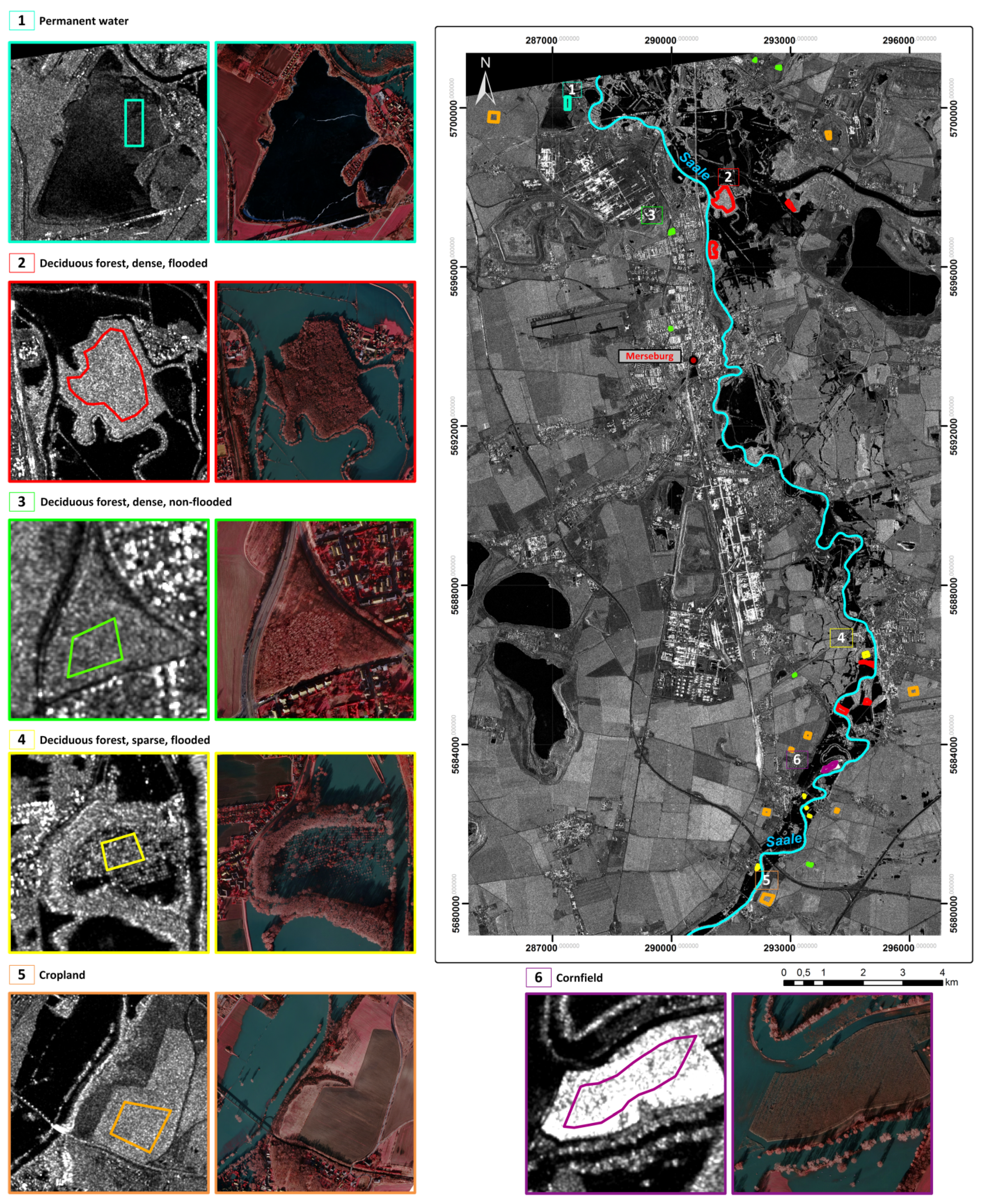
Figure 1. Study area at River Saale in Saxony-Anhalt, Germany, and visualization of test classes (polygons) in TerraSAR-X data (17 January 2011, © DLR 2014) and aerial photographs (17 January 2011 © LHW 2011).

Figure 1. Study area at River Saale in Saxony-Anhalt, Germany, and visualization of test classes (polygons) in TerraSAR-X data (17 January 2011, © DLR 2014) and aerial photographs (17 January 2011 © LHW 2011).

2.1. Study Area

The study was conducted along the River Saale located in Saxony-Anhalt, Germany, which was recently affected by floods in January 2011 and June 2013. The geographic location of the study area is presented in Figure 1. The study area is mainly defined by floodplains in the Saale valley near the city of Merseburg. The region is characterized by a relatively wide floor with flat terrain; the elevation ranges from 80 to 100 m a.s.l. Holocene alluvial sediments in the floodplains and sedimentary rocks comprised of red sandstone at the valley slopes dominate the geological setting [35]. Due to the low flow gradient of the river, the soil types are dominated by haugh-loam and Gley-Vega- alluvium [34]. Because of their high agricultural potential, the soils are mainly used as arable land. Grassland areas are sporadically employed as pasturage and orchards. Furthermore, small areas of forestry can be found. Some additional test sites are located on the plateau adjacent to the east and west of the Saale valley. These areas are dominated by loess and black earth soils which are mainly used for agriculture [35].

In the local region, the subcontinental climate is characterized by moderate temperatures and precipitation of approximately 500 mm per year [35]. The vegetation period (growing season) occurs between May and July. The tree vegetation in the regularly inundated areas of the flood plain is mainly composed of deciduous species typical of riparian woodlands, including English oak, field- and fluttering elm, and common ash [34]. The slopes and the sparsely wooded plateau are characterized by a gradual transition into lime-rich sessile oak-hornbeam forests.

The fluvial regime of the study area is dominated by the Saale main channel with contributions from both River Luppe and River Weiße Elster in the north. The River Saale and its tributaries are regularly affected by winter and summer floods. Heavy precipitation in the catchment area and temperature induced snowmelt can lead to strong water level fluctuations. In particular, the areas to the east and north of the city of Merseburg are prone to flooding [34]. Here, the distributary and backwaters of the Saale, together with various small streams and canals, shape the riparian landscape and lead to a rapid distribution of the flood water.

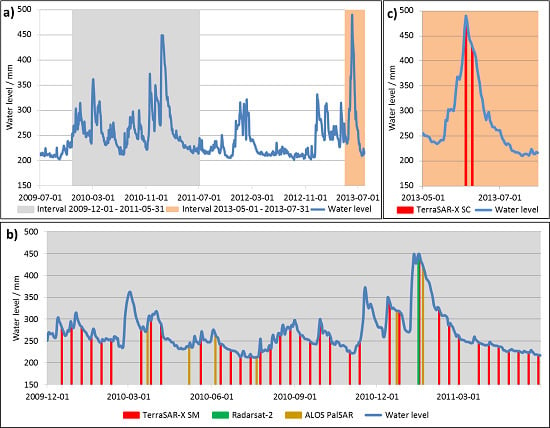
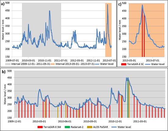
Figure 2 illustrates a time series of daily water level measurements at the Saale gauging station Rischmuehle (in Merseburg) over the period 1 July 2009 to 31 July 2013. The flood in January 2011 was caused by a particular sequence of events. Persistently heavy rainfall from August to December 2010 in central Germany led to a sharp rise in groundwater levels in the Saale catchment area. Unusually heavy snowfall in mid-December 2010, followed by several short melting periods and renewed rainfall events led to a strong rise of river levels and the subsequent flooding [36]. Intensive large-scale and continuous rainfall in central Germany and the Czech Republic through May 2013 were responsible for flood occurrences in early June 2013. Despite the high seasonal water demand of developing vegetation, the soils were quickly saturated, which led to increased direct runoff [37].

2.2. Data Set

The multi-temporal backscatter analysis is accomplished by using multi-frequency SAR data (see Table 2): The largest time-series is based on 39 TerraSAR-X HH-polarized data (λ: 3.1 cm) covering the time interval December 2009 to June 2013. The first 37 data takes are acquired in Stripmap mode (SM) (17 December 2009 to 29 May 2011) with a pixel spacing of 3.0 m. This X-band time series is supplemented by 2 TerraSAR-X ScanSAR (SC) data (pixel spacing: 8.25 m) acquired in June 2013. Due to the various number of acquisition parameters of TerraSAR-X and the non-systematic acquisition plan of the sensor such a time series is rarely available. Furthermore, as this time series covers two flood situations in January 2011 and June 2013, the data sets are predestined to analyze various semantic classes dependent on seasonal effects—especially flooded vegetation areas during leaf-on and leaf-off conditions.

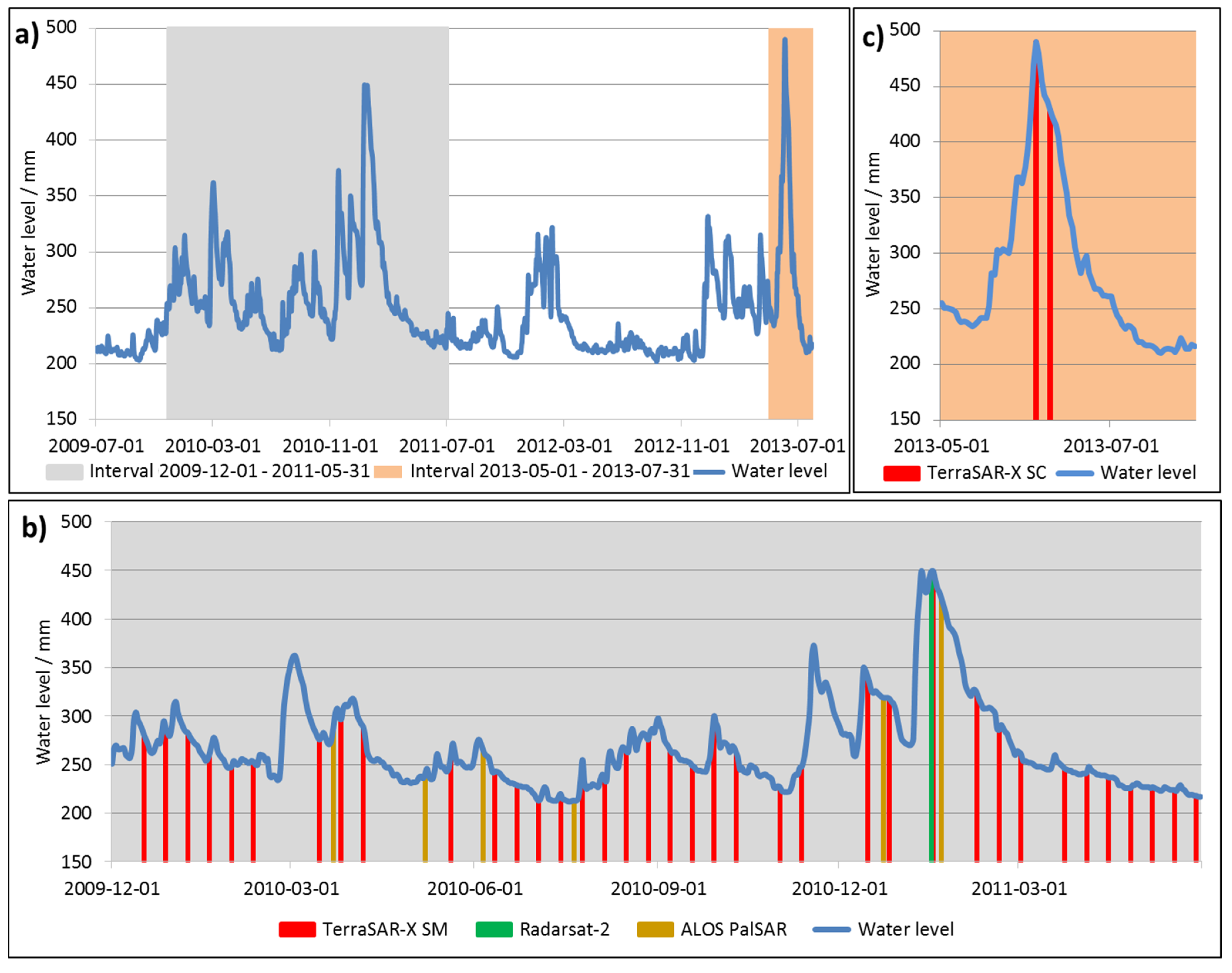
Figure 2. (a) Visualization of the water levels at gauging station Rischmuehle at River Saale for the period 1 July 2009 to 31 July 2013; (b) SAR acquisition dates and water levels at gauging station Rischmuehle for the period 1 December 2009 to 31 May 2013 and (c) 1 May 2013 to 31 July 2013.

Figure 2. (a) Visualization of the water levels at gauging station Rischmuehle at River Saale for the period 1 July 2009 to 31 July 2013; (b) SAR acquisition dates and water levels at gauging station Rischmuehle for the period 1 December 2009 to 31 May 2013 and (c) 1 May 2013 to 31 July 2013.

The X-band backscatter effects are compared to multi-temporal L-band (λ: 23.5 cm) ALOS PALSAR data acquired in Fine Beam Single (FBS; pixel spacing: 6.25 m) and Fine Beam Dual (FBD; pixel spacing: 12.5 m) mode and C-band (λ: 5.6 cm) RADARSAT-2 data acquired in Fine Beam mode (F, pixel spacing: 6.25 m). Data of both sensor types cover the flood event in January 2011 during the leaf-off phase, but not the inundation event in June 2013.

Data sets of all sensors are acquired in ascending orbit direction within nearly the same incidence angle range (see Table 2). Therefore, the influence of the sensor geometry on the backscatter analysis can be neglected. Only the TerraSAR-X SC data of 9 June 2013 are acquired with larger off-nadir angle.

For validation purposes of the SAR backscatter analysis and selection of useful test classes, the following data sets are used: Water level data of the gauging station Rischmuehle/Saale (German Federal Institute of Hydrology) for the time interval 1 July 2009 to 31 July 2013, a high resolution LiDAR-DEM as well as in-situ photographs of selected test classes acquired during a validation campaign in August 2013. Additionally, color infrared (CIR) aerial optical imagery of the flood plain with a spatial resolution of 0.5 m acquired on 17 January 2011 is at our disposal. These reference data sets are acquired on the same day as the TerraSAR-X scene and have an offset of −1 day to the RADARSAT-2 and +4 days to the ALOS PALSAR scene.

The acquisition dates of the SAR data and the water level over time are visualized in Figure 2.

Table 2. Acquisition parameters of SAR data analyzed in this case study including (Pol. = polarization, Inc. angle = incidence angle). Data sets acquired during flood events are marked in bold.

Sensor Type	Mode	Pol.	Inc. Angle Range	Product Type	Acquisition Date
TerraSAR-X	SM	HH	31.7–33.6	EEC	2009-12-17, 2009-12-28, 2010-01-08,
					2010-01-19, 2010-01-30, 2010-02-10,
					2010-03-15, 2010-03-26, 2010-04-06,
					2010-05-20, 2010-06-11, 2010-06-22,
					2010-07-03, 2010-07-14, 2010-07-25,
					2010-08-05, 2010-08-16, 2010-08-27,
					2010-09-07, 2010-09-18, 2010-09-29,
					2010-10-10, 2010-11-01, 2010-11-12,
					2010-12-15, 2010-12-26, 2011-01-17,
					2011-02-08, 2011-02-19, 2011-03-02,
					2011-03-24, 2011-04-04, 2011-04-15,
					2011-04-26, 2011-05-07, 2011-05-18, 2011-05-29
TerraSAR-X	SC	HH	31.7–40.4,	EEC	2013-06-04, 2013-06-09
			43.3–50.5
ALOS PALSAR	FBS	HH	31.6–36.8	Level 1.5	2010-03-22, 2010-12-23, 2011-01-21
ALOS PALSAR	FBD	HH/VV	31.6–36.8	Level 1.5	2009-12-03, 2010-05-07, 2010-06-05, 2010-07-21
RADARSAT-2	Fine	HH	30.2–33.6	SGF	2011-01-16

Table 2. Acquisition parameters of SAR data analyzed in this case study including (Pol. = polarization, Inc. angle = incidence angle). Data sets acquired during flood events are marked in bold.

Sensor Type	Mode	Pol.	Inc. Angle Range	Product Type	Acquisition Date
TerraSAR-X	SM	HH	31.7–33.6	EEC	2009-12-17, 2009-12-28, 2010-01-08,
					2010-01-19, 2010-01-30, 2010-02-10,
					2010-03-15, 2010-03-26, 2010-04-06,
					2010-05-20, 2010-06-11, 2010-06-22,
					2010-07-03, 2010-07-14, 2010-07-25,
					2010-08-05, 2010-08-16, 2010-08-27,
					2010-09-07, 2010-09-18, 2010-09-29,
					2010-10-10, 2010-11-01, 2010-11-12,
					2010-12-15, 2010-12-26, 2011-01-17,
					2011-02-08, 2011-02-19, 2011-03-02,
					2011-03-24, 2011-04-04, 2011-04-15,
					2011-04-26, 2011-05-07, 2011-05-18, 2011-05-29
TerraSAR-X	SC	HH	31.7–40.4,	EEC	2013-06-04, 2013-06-09
			43.3–50.5
ALOS PALSAR	FBS	HH	31.6–36.8	Level 1.5	2010-03-22, 2010-12-23, 2011-01-21
ALOS PALSAR	FBD	HH/VV	31.6–36.8	Level 1.5	2009-12-03, 2010-05-07, 2010-06-05, 2010-07-21
RADARSAT-2	Fine	HH	30.2–33.6	SGF	2011-01-16

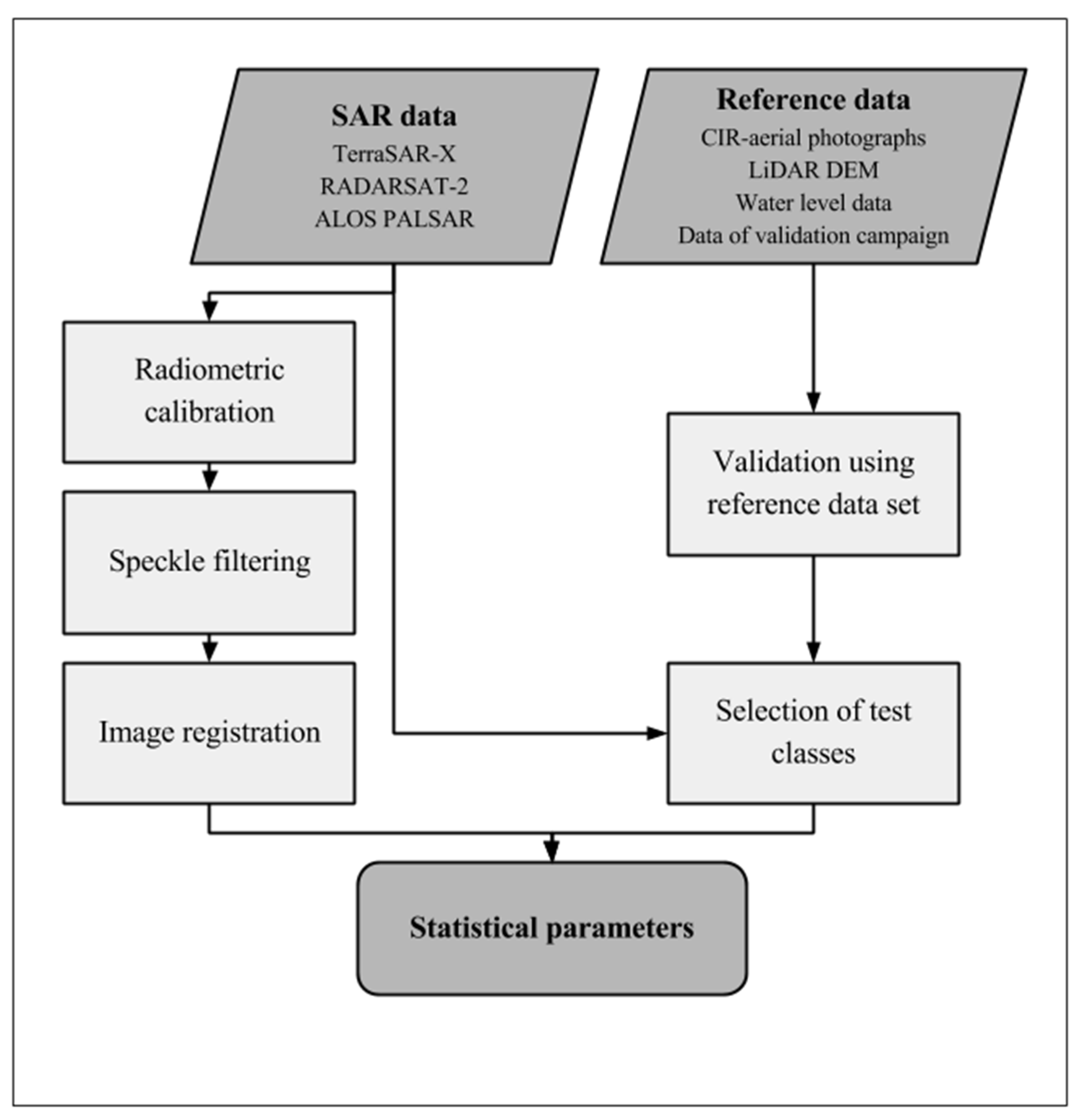
2.3. Preprocessing: SAR-Calibration, Speckle-Filtering and Image Registration

The workflow of the data preprocessing is visualized in Figure 3. The SAR data sets were converted to sigma nought (σ₀) values (dB) to ensure that images obtained from different sensors and acquisition modes were statistically comparable [38]. The radiometrically calibrated values represent the normalized radar cross section and describe radar reflectance properties per pixel. The data calibration compensates for the radiometric influences of different incidence angles (caused by the sensor geometry and topographic characteristics of the surface).

The TerraSAR-X scenes (SM and SC) were calibrated using the TerraSAR-X Flood Service (TFS) developed by the German Remote Sensing Data Center (DFD) for the German Aerospace Center (DLR) [4]. For the calibration process of the 39 Stripmap scenes the Geocoded Incidence Angle Mask (GIM) created by the data provider was used. The calibration and subsequent speckle filtering of the RADARSAT-2 and ALOS PALSAR scenes was carried out with the Next ESA SAR Toolbox software 5.1 (NEST). Speckle is a typical phenomenon of random, high-frequency noise in SAR images that results from many randomly distributed point scatterers in a resolution cell. To resemble the demand for processing efficiency and the conditions of DLR’s TerraSAR-X Flood Service, a 3 × 3 median filter was chosen. The median filter reduces the high frequency image structure. The same filter configuration was applied to the remaining SAR data sets.

Figure 3. Workflow for time-series analysis.

Figure 3. Workflow for time-series analysis.

To ensure the most exact pixel overlap of the different data sets, subsets of RADARSAT-2 and ALOS PALSAR data were registered on the geometry of the TerraSAR-X scenes using the software Exelis Envi 5.0. Matching control points between the TerraSAR-X reference scene (17 January 2011) and the respective slave scenes were established. These are based on easily recognizable structures such as bridges or street intersections. With regard to the following statistical analysis the registration was carried out using a nearest neighbor function to preserve the original pixel values. Due to the high positional accuracy of the TerraSAR-X sensor and the almost identical imaging geometry, coregistration of the TerraSAR-X data sets was not required.

2.4. Selection and Statistical Analysis of Test Areas

The statistical analysis of the time series data was performed for six test classes, each consisting of several test areas (Figure 1). The test polygons were manually digitized after detailed review of the available data sets (see Chapter 2.2) and validated with field observations in August 2014. The selection of the six test classes and individual test sites was limited by the small-scale dimensions of the geographic setting in the region, defined by a mixture of urban, cropland, forest, and river-floodplain landcover. Each of the selected test classes consists of several test sites with relatively homogenous surface characteristics. Anthropogenic objects and widely differing types of vegetation cover were excluded. To further eliminate or reduce the influence of radar shadow effects, especially at the edge of forested areas, the outline of the polygons was set at an appropriate distance from edges of homogenous areas. Despite significant generalization of the land cover, the Corine Land Cover 2006 (100 m resolution) data set and the topographic map of Saxony-Anhalt (scale 1:10,000 m) helped with the initial identification of the dominant land cover and vegetation types within the study area. Digitization was primarily based on aerial photographs captured on 17 January 2011 and supported by various SAR scenes and the use of a high-resolution LiDAR-DEM to estimate the expected flood level. A sample polygon of each object class in TerraSAR-X data (17 January 2011) and aerial photographs (17 January 2011) is illustrated in Figure 1.

Test class 1 (size: 3.56 km², 3 polygons) consists of permanent waterbodies which are rarely influenced by wind induced roughness effects and seasonal freezing. To eliminate the effects of inflows, riparian vegetation and water level changes only big, isolated water bodies were selected. Several areas of deciduous dense forests were separated in occasionally flood affected (class 2, size: 0.33 km², six polygons) and perennial non-flood affected (class 3, size: 0.31 km², six polygons) test sites. Both are covered by trees with an approximate height of 20 to 25 m and show a dense canopy. To further estimate the influence of tree density and habitus a 4th test class (size: 0.02 km², six polygons) containing flood affected sparse deciduous forests was selected. These 5 to 8 m high orchard trees have varying canopy sizes. There are partly wide gaps of approx. 20 to 20 m in between the tree communities (7–12 m trunk distance). Test class 5 (size: 0.61 km², 10 polygons) consists of non-flooded cropland with crop, maize and various field crops. The actual field cover and growing state during the study period could not be verified. A single, partially flooded maize field, which shows noticeable high radar backscatter was selected for test class 6 (size: 0.03 km², 1 polygon). The smallest test area (class 3) contains 2645 pixels, the largest test area (class 1) 470,743 pixels in TerraSAR-X SM data.

For each test class, several statistical parameters of σ₀ were calculated. Based on the test area polygons, the mean, median, minimum, maximum value and standard deviation were derived.

3. Results and Discussion

The following section highlights significant trends and extreme values in the time course of the radar backscatter. Possible influences on the scattering processes of the X-, C- and L-band sensors by system and environmental parameters are considered. Furthermore, the ability of TerraSAR-X to detect flooding under vegetation will be compared with C- and L-band sensors and discussed in the context of the findings of other studies. The Figure 4, Figure 5, Figure 6, Figure 8, Figure 9 and Figure 10 show mean and standard deviation of σ₀ (dB) for all six test classes over the time course of the study period. A closed and a dashed line are used in the figures to link the mean and the standard deviation, respectively, to facilitate the interpretation of the trend lines. The lines do not represent an interpolation between the measurements.

Permanent water (test class 1) shows a strong fluctuation of σ₀ in X-band over the entire course of the time series (Figure 4). The mean backscatter varies between −27.08 dB and −17.27 dB. As all data are acquired within the same incidence angle range this fluctuation can be related to different surface roughness conditions due to wind effects and seasonal freezing. Accordingly, the fluctuation of the mean backscatter in L-Band (−20.45 dB to −15.96 dB) is lower than in X-band. Bright backscattering caused by the Bragg effect which may occur in dependence of the sensor’s wavelength and incidence angle on periodically spaced surface patterns such as waves on water surfaces does not occur in the data. This phenomenon may reduce the separability of open water, flooded vegetation and non-water areas.

Figure 4. Time course of σ₀ (dB): Mean and standard deviation for test class 1 (Permanent water).

Figure 4. Time course of σ₀ (dB): Mean and standard deviation for test class 1 (Permanent water).

The optimum threshold value to separate permanent water areas (class 1) and non-water areas (combined classes 3 and 5) of all data sets are computed based on the calculation of the Overall Accuracy (OA) for the backscatter range between −40 to 0 dB (Δ0.25 dB). The mean optimum threshold value is −13.4 dB for the X-band time series and −14.3 dB for the L-band data. The high standard deviation of the optimum threshold value (2.3 for X-band, 2.2 for L-band) as well as the high variability of the backscatter shows that in water and flood detection applications, a threshold for separating water and non-water areas has to be set individually for each scene, especially for X-band data. Empirically predefined threshold values could lead to a significant misclassification of the water extent. Noticeable peaks of standard deviation around February 2010 and January 2011 are caused by partial ice cover of the permanent water bodies. Due to increased surface roughness, ice causes much stronger backscattering in comparison to smooth open water bodies.

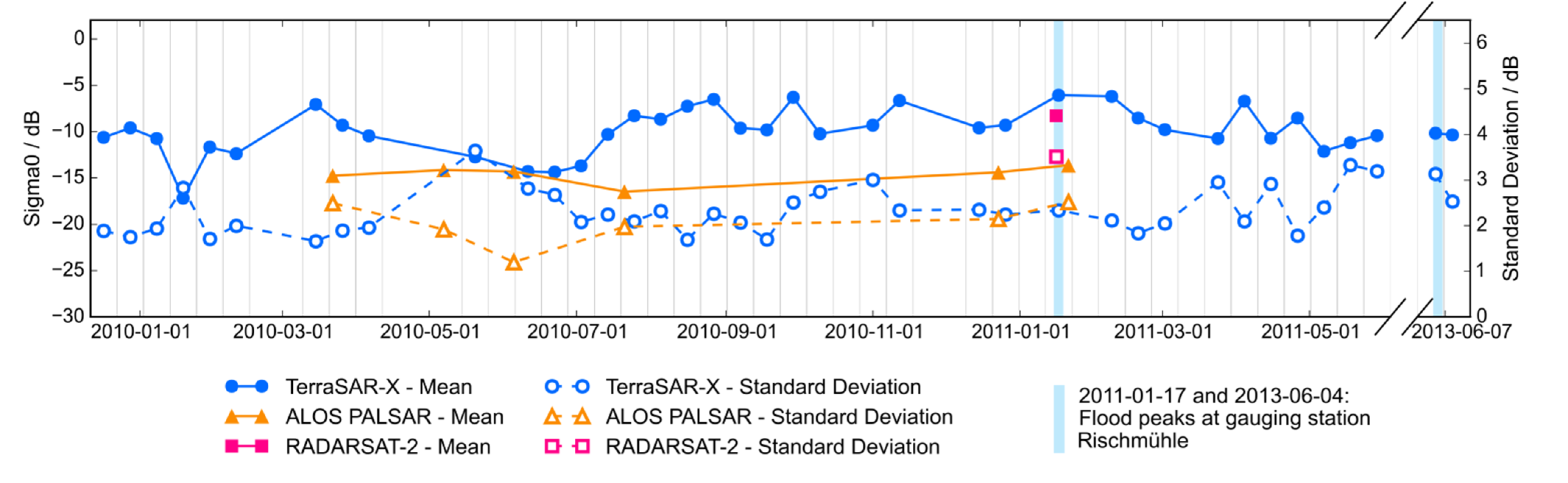
Outside the flooding periods, the statistical characteristics of the flooded and non-flooded test classes of dense, deciduous forest show a high degree of conformity in X-, C-, and L-Band due to similar vegetation conditions (see Figure 5 and Figure 6). The start of the vegetation period coincides with a rise of standard deviation in X-band (Figure 5). The developing canopy increases the amount of diffuse volume scattering. Figure 6 is showing a less distinct increase, which can be attributed to slightly different canopy density and geometric structure of the tree species composition at the non-flood affected test sites. The development of backscatter and standard deviation over the time course is even more similar for L-Band wavelengths. Higher penetration depth leads to less dependency of the scattering mechanisms on the structure and seasonal development of the tree canopy.

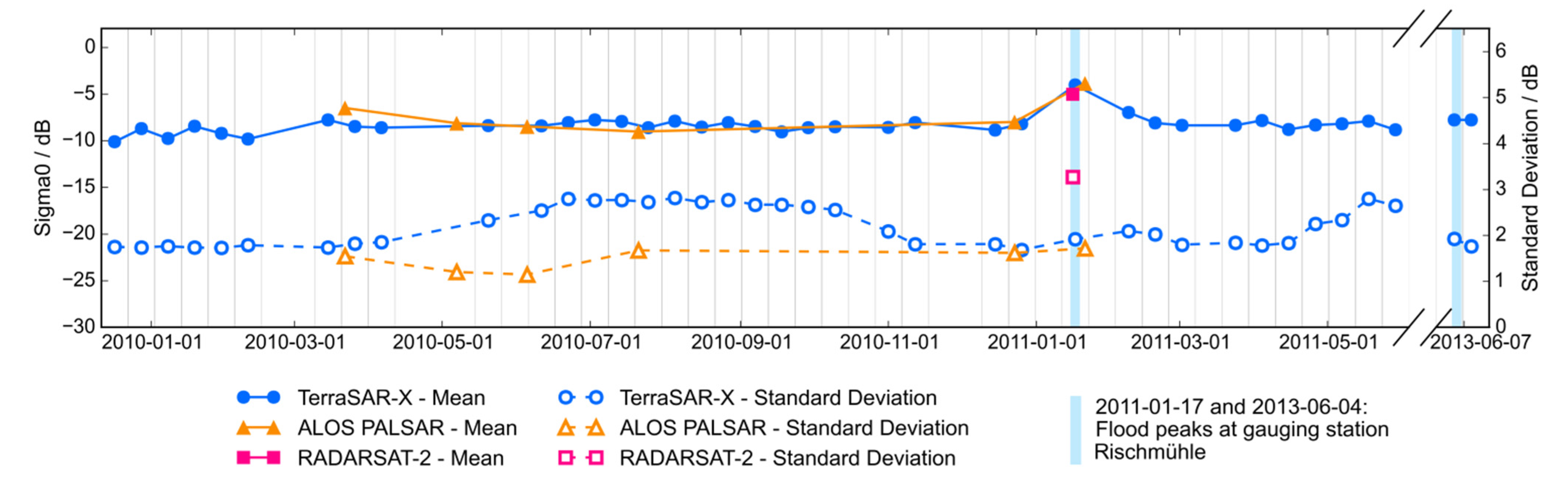
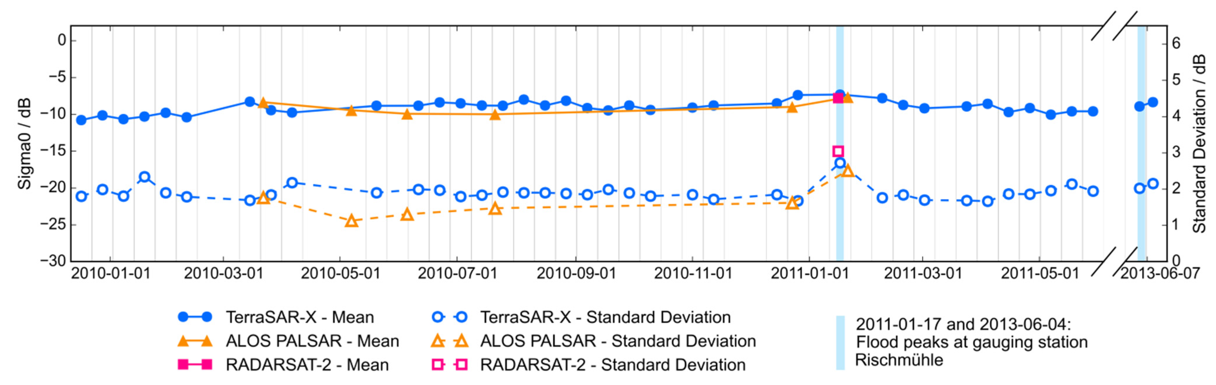
During the flood event in January 2011, class 2 (Figure 5) shows similar mean backscatter in X- (−4.06 dB), C- (−5.02 dB), and L-band (−3.87 dB) data. These values differ clearly from the homogenous backscatter profiles and their time course mean in X- (−8.48 dB) and L-Band (−8.10 dB) of class 2 during non-flood conditions (excluding January 2011). In comparison to these results and the corresponding January 2011 data of class 3 (−8.33 dB in X-Band) an increase in X-Band of 4.42 dB resp. 4.27 dB caused by strong double bounce scattering under flood conditions can be observed. This confirms the findings of previous studies that flooded vegetation can—at least under leaf-off conditions of deciduous vegetation—be reliably detected with X-band sensors: The backscatter increase of Δ4.42 dB over flooded deciduous leaf-off forest compared to the mean TerraSAR-X time course (min: Δ2.94 dB, max Δ6.25 dB) is nearly as high as Voormansik et al. (2014) [20] determined for a study area in Estonia (6.2 dB). In comparison, Pulvirenti et al. (2013) [22] reported increased backscattering of Δ7.0–8.6 dB over flood surfaces covered by olive groves and deciduous forests in Italy using Cosmo-SkyMed data. Martinis et al. (2015) [24] stated a backscatter increase of up to Δ7.5 dB over grassland and foliated shrubs in Caprivi/Namibia in comparison to pre-flood conditions.

Figure 5. Time course of σ₀ (dB): Mean and standard deviation for test class 2 (Deciduous forest, dense, flooded).

Figure 5. Time course of σ₀ (dB): Mean and standard deviation for test class 2 (Deciduous forest, dense, flooded).

Figure 6. Time course of σ₀ (dB): Mean and standard deviation for test class 3 (Deciduous forest, dense, non-flooded).

Figure 6. Time course of σ₀ (dB): Mean and standard deviation for test class 3 (Deciduous forest, dense, non-flooded).

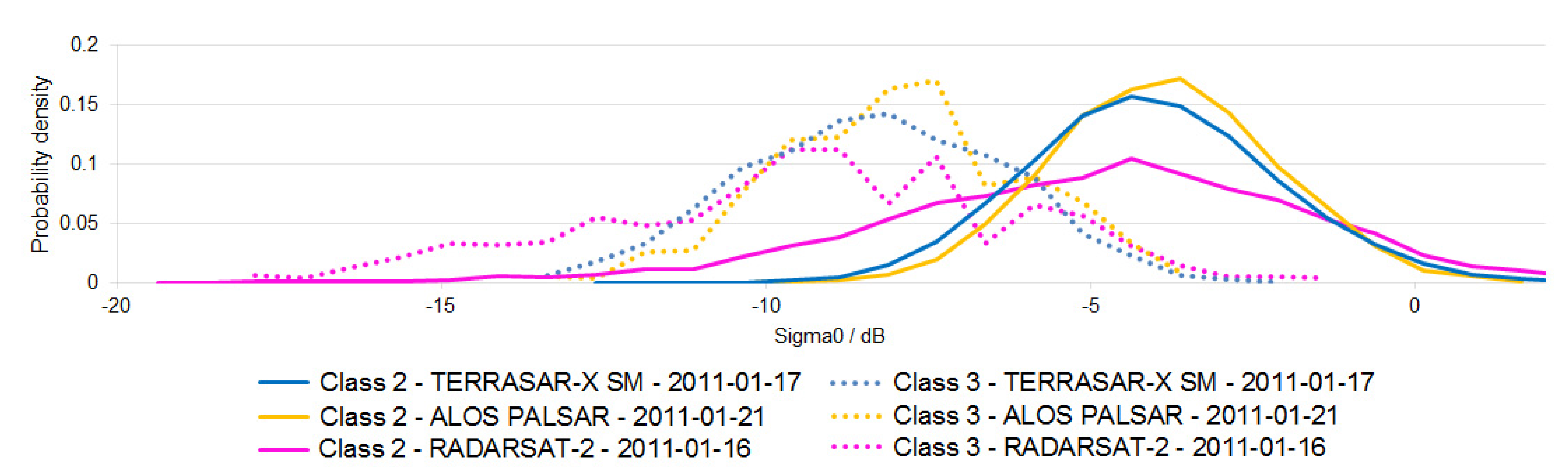
In L-Band a similar backscatter difference during flooded conditions of 4.23 dB compared to the class 2 non-flooded time series mean resp. 4.11 dB to the class 3 January 2011 data can be observed. The histograms of class 2 and 3 for X- (17 January 2011), C- (16 January 2011) and L-Band (21 January 2011) are nearly Gaussian distributed (see Figure 7). The probability density of the histograms was calculated for 60 categories between a backscatter range of −40 and +5 dB and normalized due to different pixel size of the different sensor data. To compare the separability of the two classes for all sensors, the M-statistic [39] is computed as $\left|{\text{μ}}_1-{\text{μ}}_2\right|/{\text{σ}}_1-{\text{σ}}_2$, where ${\text{μ}}_1$ and ${\text{μ}}_2$ are the mean values and ${\text{σ}}_1\text{ and }{\text{σ}}_2$ are the standard deviations of class 2 and class 3, respectively. The best separability have the probability density functions of the ALOS PALSAR data (0.53), followed by slightly lower values for TerraSAR-X (0.48), and significantly lower values for RADARSAR-2 (0.18).

Figure 7. Histograms of class 2 and 3: TerraSAR-X SM (17 January 2011), ALOS PALSAR (21 January 2011), and RADARSAT-2 (16 January 2011).

Figure 7. Histograms of class 2 and 3: TerraSAR-X SM (17 January 2011), ALOS PALSAR (21 January 2011), and RADARSAT-2 (16 January 2011).

In contrast to the above described good separability in January 2011, the TerraSAR-X ScanSAR data of 4 June 2013 only shows a relatively small shift for class 2 of mean σ₀ to −7.78 dB. In direct comparison to the corresponding class 3 value (−8.54 dB) and the time series mean of the TerraSAR-X Stripmap data under non-flood conditions (−8.48 dB), the backscatter increases by only 0.76 dB resp. 0.7 dB. The limited ability of X-Band to penetrate the dense summer foliage leads to dominating diffuse volume scattering. Without a strong backscatter increase due to additional double-bounce interaction with the water surface, the separation of partially flooded and non-flooded areas of vegetation cover is not possible.

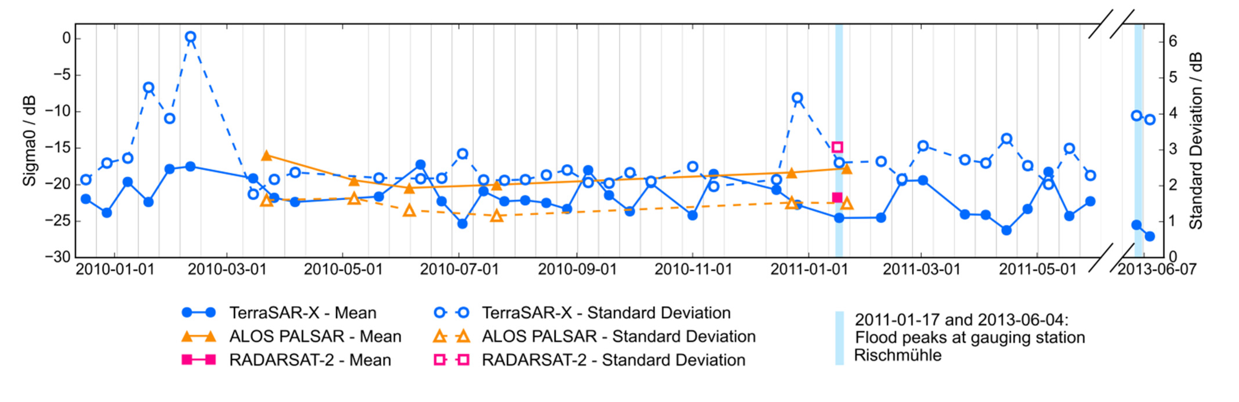
Despite different tree density and species composition, class 4 (Figure 8) is showing very similar time series characteristics as the dense forest test classes. During the flooding in January 2011, the absolute mean backscatter values are comparable among each other in X- (−7.33 dB), C- (−7.8 dB), and L-band (−7.69 dB) data. The increase in radar backscatter in comparison to the respective time course mean under non-flooded conditions (excluding January 2011) is not very distinct in X- (Δ1.81 dB) and L-band (Δ1.61 dB). The backscatter mean only slightly increases as class 4 consists of single trees with trunk distances around 7 to 12 m to each other, partially interrupted from wide gaps of approx. 20 to 20 m. Bright backscattering due to double bouncing on the flooded vegetation is therefore nearly compensated by SAR shadowing effects as well as specular reflection on open water surfaces. However, these phenomena lead to a noticeable increase of the standard deviation of the backscatter within the test areas in X- and L-band data which could be used as an indicator for detecting partially submerged vegetation.

Figure 8. Time course of σ₀ (dB): Mean and standard deviation for test class 4 (Deciduous forest, sparse, flooded).

Figure 8. Time course of σ₀ (dB): Mean and standard deviation for test class 4 (Deciduous forest, sparse, flooded).

In comparison to the class 2 time series mean of the standard deviation under non-flooded conditions (X-Band: 1.87 dB; L-Band: 1.48 dB), the standard deviation for January 2011 (X-Band: 2.73 dB; L-Band: 2.51 dB) increases about 0.86 dB in X-Band and 1.03 dB in L-Band. The use of the standard deviation in flood mapping algorithms cannot be applied in pixel-based applications. It requires the calculation of this parameter over a certain area of the SAR scene e.g., using a moving window, pre-defined polygons based on landcover information or object based algorithms, which apply classification algorithms on segments created according to defined homogeneous criteria [40].

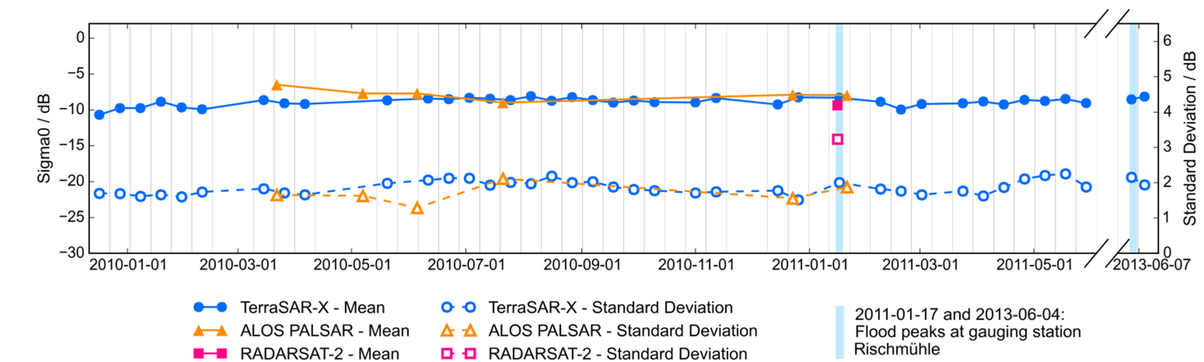
Both the mean backscatter and the standard deviation of non-flooded cropland (class 5) are very heterogeneous over the time series (Figure 9). This is related to several factors such as differences in soil moisture, plant phenological stages, and furrow orientation as well as variations of the crop type over time. The values of mean σ₀ are much higher and the backscatter variations are much more pronounced in X- (−17.19 to −6.08 dB) than in L-band (−16.49 to −13.63 dB). Cropland is one of the most difficult classes for detecting standing water beneath the vegetation as backscatter changes are often erroneously connected with strong backscatter effects of other classes. The high variability of this class requires very strong backscatter increases in comparison to pre-event data and absolute backscatter values > −5 dB in X- and > −10 dB in L-band.

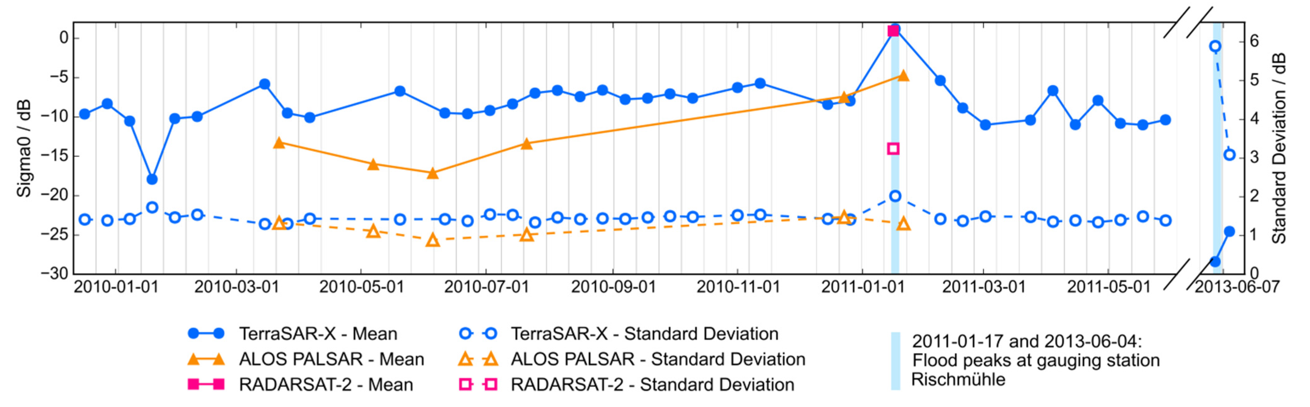
A good example is visualized in Figure 10 which shows the statistical analysis of a single cornfield (class 6). The field is covered by maize.

Figure 9. Time course of σ₀ (dB): Mean and standard deviation for test class 5 (Cropland, non-flooded).

Figure 9. Time course of σ₀ (dB): Mean and standard deviation for test class 5 (Cropland, non-flooded).

Figure 10. Time course of σ₀ (dB): Mean and standard deviation for test class 6 (flooded cornfield).

Figure 10. Time course of σ₀ (dB): Mean and standard deviation for test class 6 (flooded cornfield).

The temporal backscattering over maize is highly variable in X-band data. This was also stated by e.g., [41] using ERS-1 C-band data. This cannot be explained by the evolution of the crop biophysical parameters. Due to the structure of its canopy, maize is one of the most transparent crops to the SAR signal even at fully developed stages [39] and therefore, the SAR backscatter is strongly influenced by soil moisture properties [42]. The test area is partially flooded in January 2011 and therefore gives a very bright backscatter signal in both X- and C-band of 1.17 dB and 0.92 dB, respectively. This corresponds to an X-band backscatter increase of 9.86 dB in comparison to the TerraSAR-X-SM time course mean under non-flooded conditions (−8.69 dB). The backscatter in L-band also shows the influence of double bounce effects with an absolute backscatter change of Δ8.58 dB. However, compared to X-band the absolute mean signal return in L-band for January 2011 is much lower (−4.70 dB). It is not easy to interpret if this phenomenon is related to the different penetration properties of L-Band or to a slight decrease in water level between the acquisitions of TerraSAR-X (17 January 2011) and ALOS PALSAR (21 January 2011) which may lead to variations of the double bounce effects. Large double bounce effects over inundated agricultural areas have also been stated in the literature. According to [5], simulations based on electromagnetic scattering models using different frequency bands (X-, C-, and L-band) have shown that the backscatter increase of agricultural cropland can become quite large (at least 2–3 dB) when the crop reached at least an intermediate stage of growth.

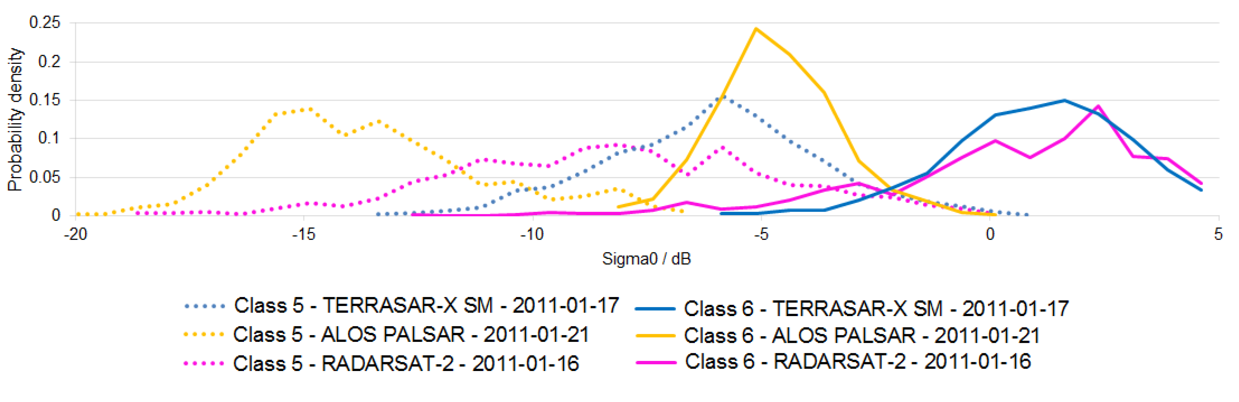
Figure 11 shows the probability densities of the histograms of non-flooded cropland (class 5) and the flooded cornfield (class 6) of all sensors during the flood event in January 2011. The positions of the respective histograms are rather similar for X- and C-band with a strong offset (>8.5 dB) towards lower backscatter values in L-band. According to the M-statisitic the best class separability is obtained by L-band data (0.91), while the probability density functions of TerraSAR-X and RADARSAT data have lower class separability with similar values of 0.28 and 0.25, respectively.

Figure 11. Histograms of class 2 and 3: TerraSAR-X SM (17 January 2011), ALOS PALSAR (21 January 2011), and RADARSAT-2 (16 January 2011).

Figure 11. Histograms of class 2 and 3: TerraSAR-X SM (17 January 2011), ALOS PALSAR (21 January 2011), and RADARSAT-2 (16 January 2011).

Due to the higher water level during the flooding in June 2013, this cornfield is nearly completely inundated on 4 June 2013 and completely covered by water on 9 June 2013. Therefore, as these areas are mainly characterized by specular reflection the absolute backscatter is < −25 dB in both TerraSAR-X ScanSAR scenes. The high standard deviation on 4 June 2013 is related to the appearance of some single flooded trees of bright backscatter which are surrounded by flat water surfaces.

The standard deviation is nearly constant over time in both TerraSAR-X SM (ca. 1.44 dB) and ALOS PALSAR data (ca. 1.17 dB). During the flooding in January this parameter increases to 2.02 dB in X-band, whereas there is no significant increase of the standard deviation in L-band.

4. Conclusions and Outlook

In this paper, an analysis of multi-temporal and multi-frequency Synthetic Aperture Radar data is performed to investigate the general backscatter behavior of several semantic classes in the context of flood mapping in central Europe. The focus is on a test area at River Saale, Saxony-Anhalt, Germany which is covered by a time series of 39 TerraSAR-X data acquired within the time interval December 2009 to June 2013 and supplemented by 7 ALOS PALSAR data and a single RADARSAT-2 scene. Within this study period, two flood events occurred in January 2011 and June 2013 which allows evaluating multi-frequency backscatter variations between flooding and normal water level conditions. The main findings are summarized in the following:

• Due to the influence of waves and seasonal freezing the variability of the backscatter over permanent open water areas (class 1) is very high (in X-band: ~Δ10 dB, in L-band: ~Δ4.5 dB). Analyses have shown that the optimum threshold value for separating open water surfaces and non-water areas has a high variability. Therefore, misclassifications can be reduced if the threshold value for separating water and non-water areas is set individually for each scene.
• Absolute values of σ₀ show nearly identical values for both flooded dense (class 2) and flooded sparse forests (class 4) during the leaf-off phase in X-, C-, and L-band. Over a partially flooded cornfield (class 6), the backscatter shows similarly strongly enhanced values in X- (1.17 dB) and C-band (0.92 dB). In L-band, however, the backscatter appears to be much lower (−4.70 dB).
• Also, the backscatter differences in X- and L-band between pre-flood and flood conditions are nearly identical for both flooded dense (class 2; X-band: Δ4.42 dB, L-band: Δ4.23 dB) and sparse forests (class 4; X-band: Δ1.81 dB, L-band: Δ1.62 dB) during the leaf-off phase. Over a partially flooded cornfield (class 6), the backscatter difference between the flooding in January 2011 and the mean backscatter of the time course under non-flooded conditions is also nearly identical (X-band: Δ9.86 dB, L-band: Δ8.58 dB).
• Under certain circumstances, X-band data could be used for the detection of standing water beneath sparse vegetation such as cornfields or beneath forests during the leaf-off phase. However, in this study, inundated dense deciduous forests during the leaf-on phase only show a minor increase in backscatter of ~ Δ0.7 dB in comparison to the time series mean of the TerraSAR-X SM data and, therefore, can hardly be detected.
• In L-band, the results offer a wide range of backscatter increases between Δ4.23 dB for inundated leaf-off forest and Δ8.58 dB for a flooded cornfield. This very heterogeneous development for L-band can also be found in the literature, with backscatter increases in L-band varying between Δ1.6 dB and Δ9.7 dB for different vegetation types according to the studies listed in Table 1.
• The standard deviation does not give auxiliary information in detecting flooded dense (class 2) deciduous forests during the leaf-off phase. However, in X- and L-band a significant increase of this parameter could be determined over sparse flooded forests (test class 4). This class is affected by strong backscatter variation due to double bounce effects on the one hand and specularly reflecting water surfaces and radar shadowing effects within vegetation gaps on the other hand. Further, significant changes in the standard deviation can be found over a cornfield in X-band between flooded and non-flooded conditions. Further investigations are necessary if this parameter can be used in addition to backscatter information for improving the detection of flooded vegetation, e.g., in object based classification algorithms.

According to the findings, there is great potential in detecting flooding beneath vegetation in all microwave wavelengths, even in X-band for sparse vegetation or leaf-off forests. However, the use of fixed empirical threshold values for automating the detection of partially submerged vegetation of various types is nearly impossible due to the dependency of the SAR signal return over partially flooded vegetation on various system and environmental parameters.

Most straightforward seem to be approaches which consider various parameters. e.g., fuzzy logic-based algorithms could be used for combining different absolute backscatter thresholds for various semantic classes (e.g., forest during leaf-off and leaf-on phase, grassland, and cropland) and change detection information based on backscatter differences between single pre-flood or time series data and the crisis image. Further, SAR data of various wavelengths, incidence angles, and polarizations could be integrated to account for different backscatter mechanisms. Most critical is the selection of pre-flood data, especially for classes of high backscatter variability such as cropland. This requires the comparison of the data to mean backscatter values of corresponding time series data sets and the limitation of false-alarms by restricting the potential of flood occurrence by e.g., topographic information sources.