
Regional Urban Extent Extraction Using Multi-Sensor Data and One-Class Classification


Abstract
:
1. Introduction
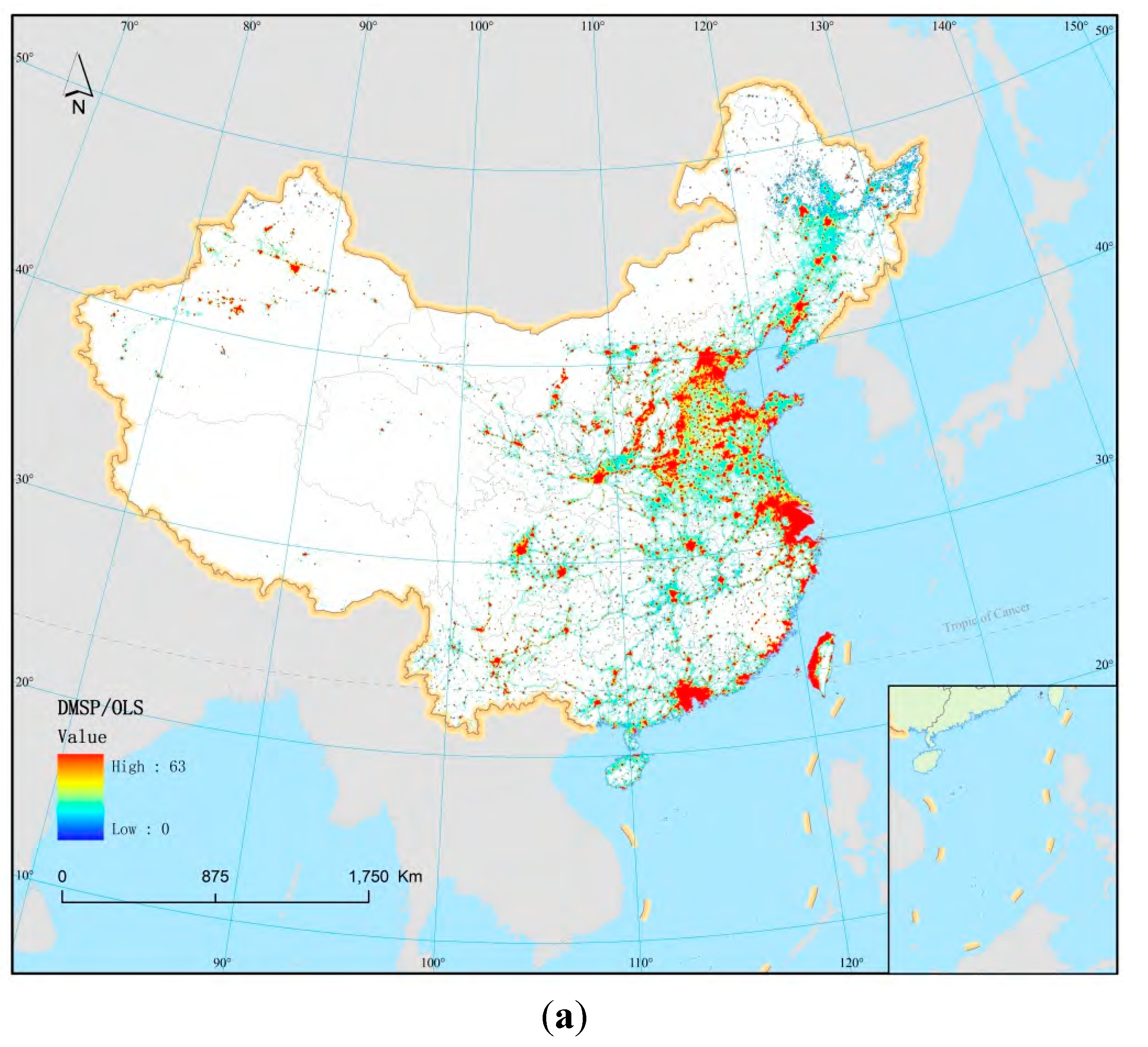
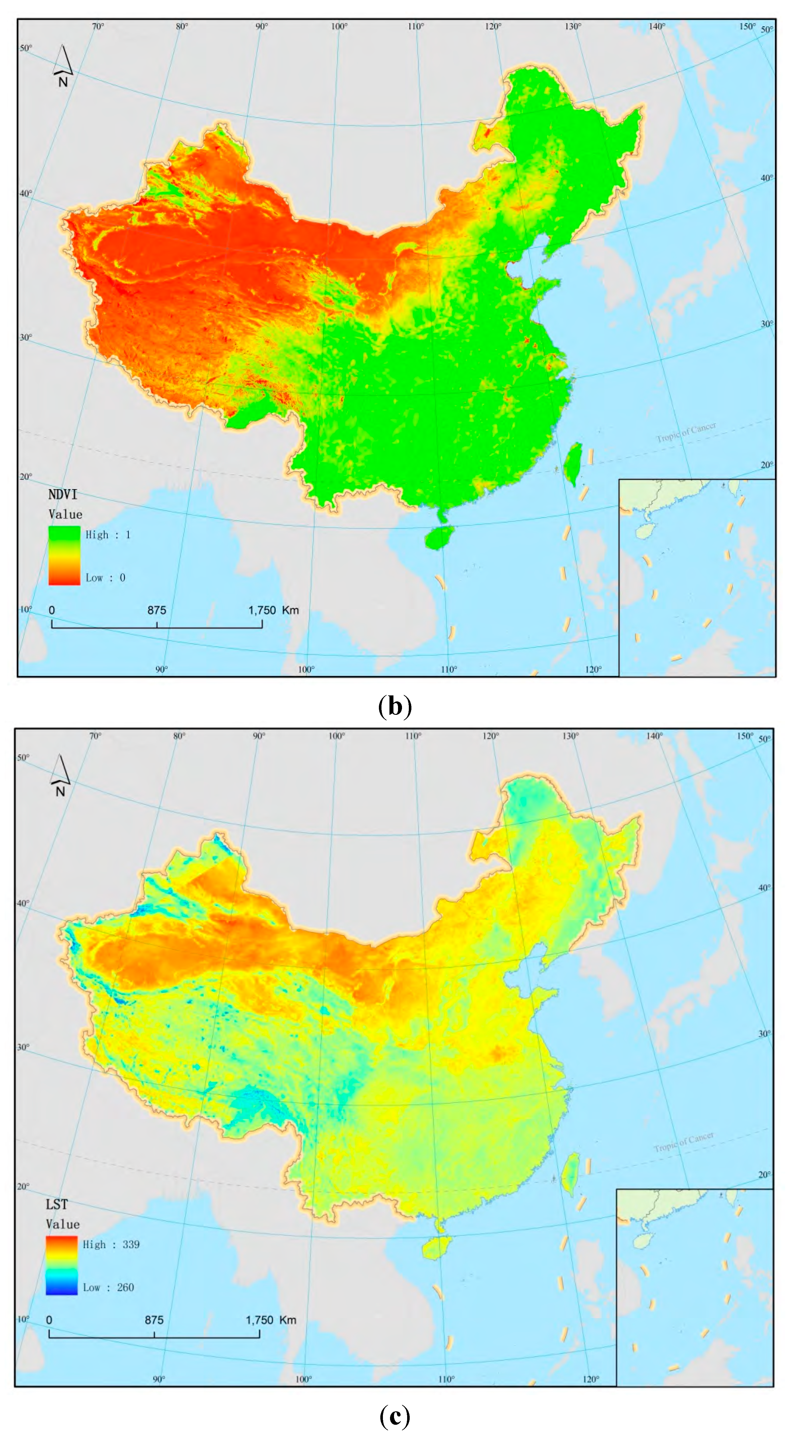
2. Study Area and Data


3. Methods
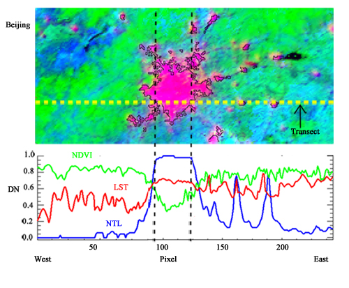
3.1. Data Analysis
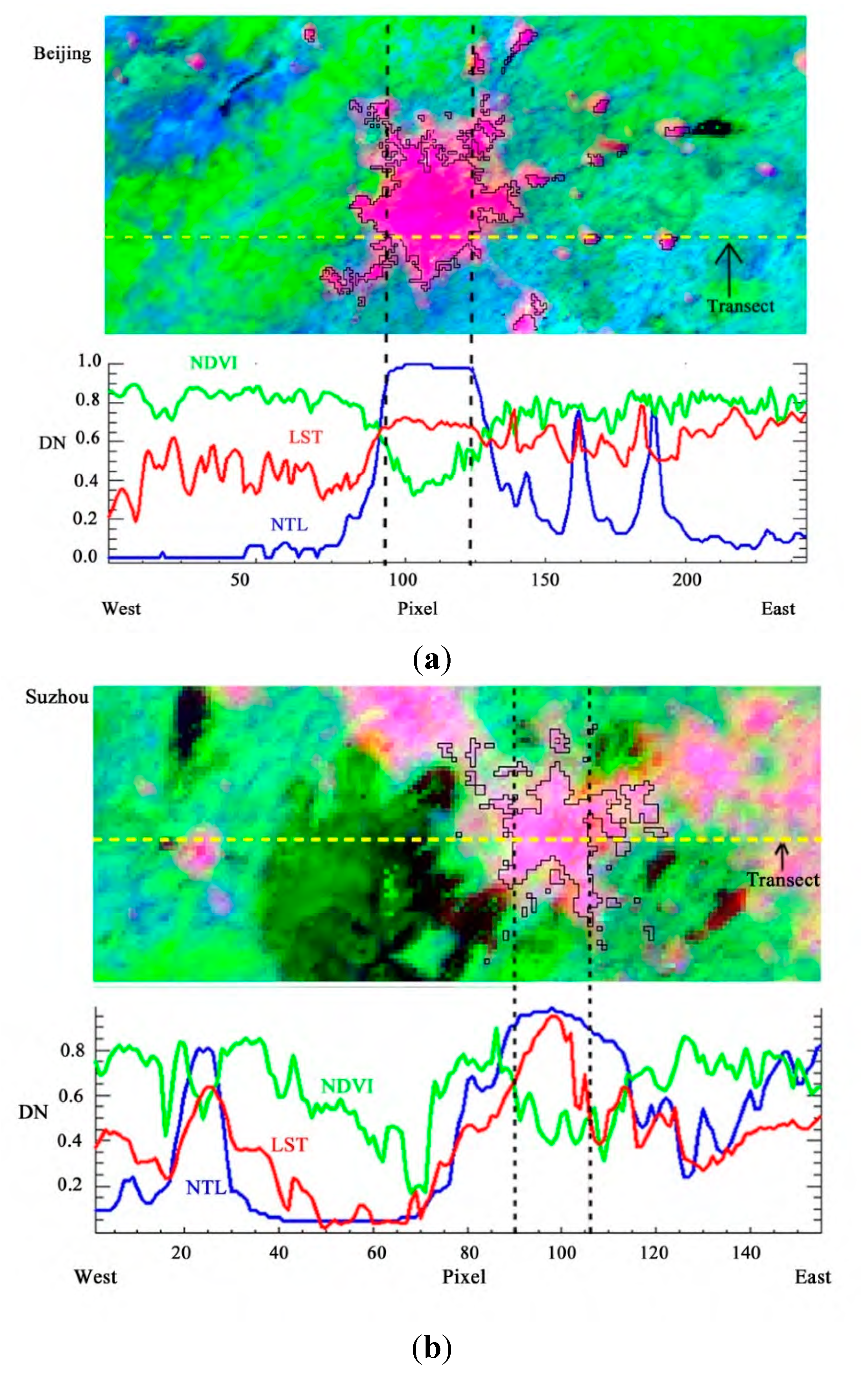
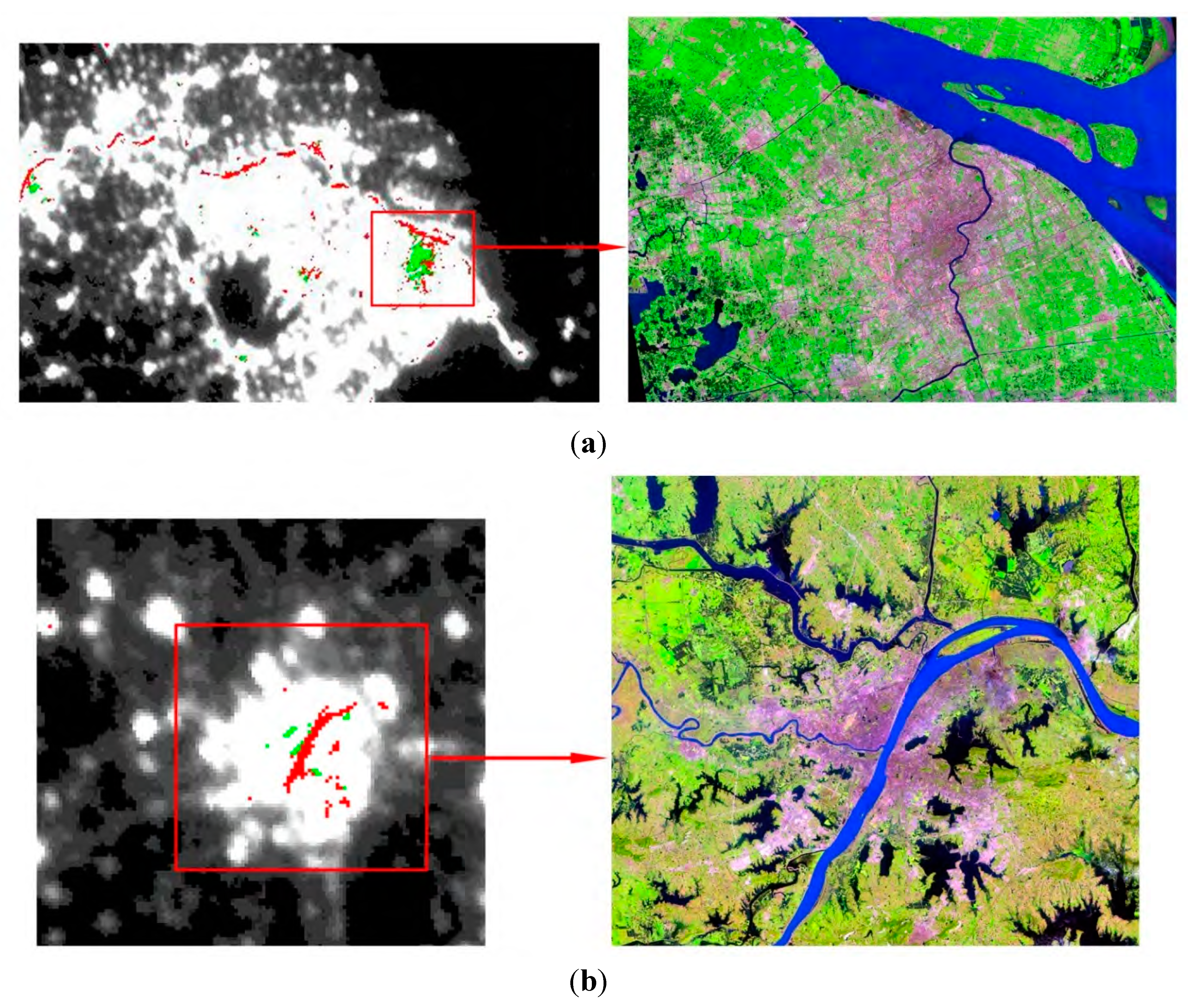
3.2. Extraction of Urban Areas Using Multiple Sensor Data
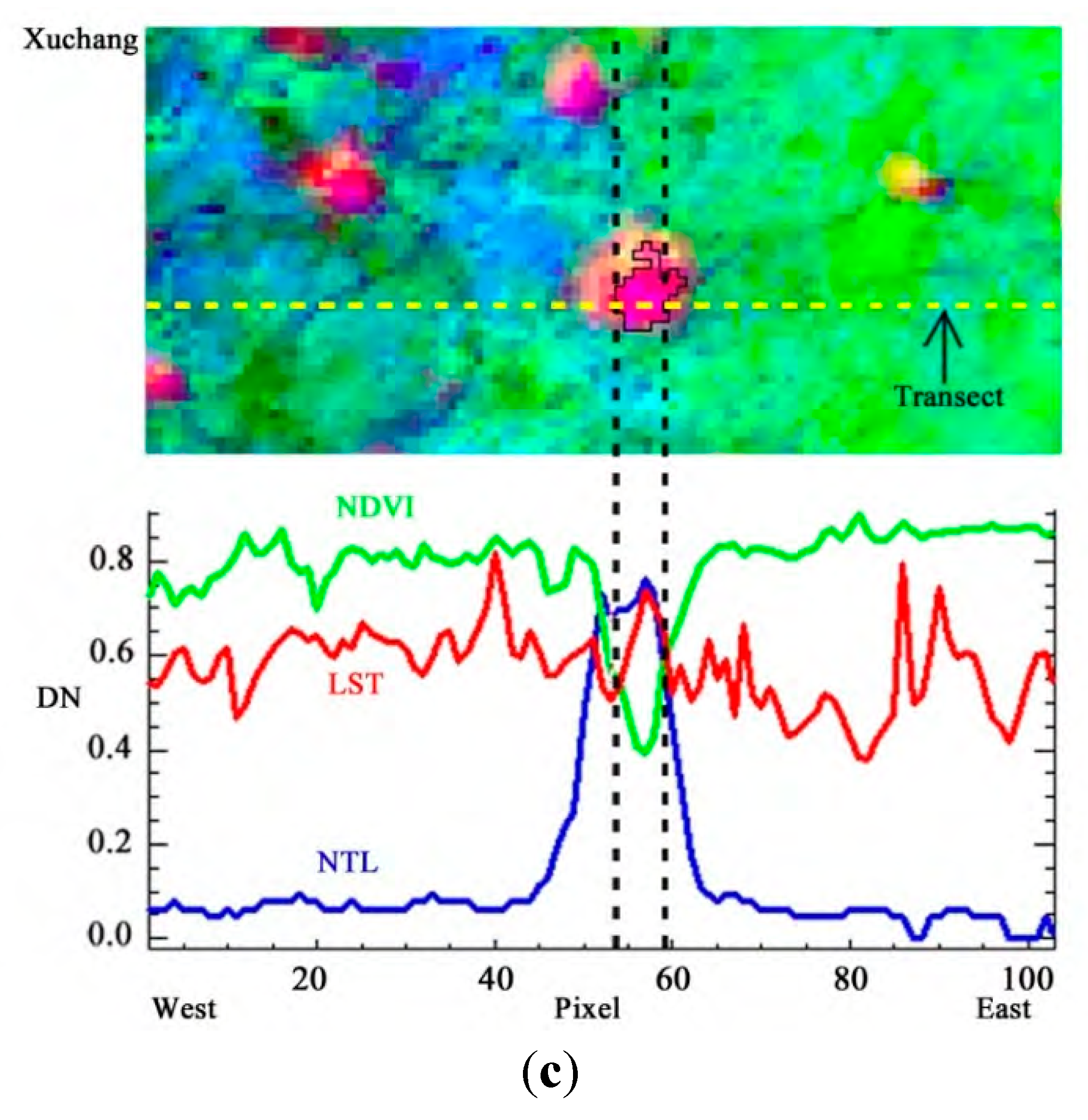
3.3. Validation
4. Results

| Local-Optimized Threshold Method | OCSVM Classification with NTL + NDVI | OCSVM Classification with NTL + LST | OCSVM Classification with NTL + NDVI + LST | |
|---|---|---|---|---|
| Beijing | 0.1642 | 0.1312 | 0.1460 | 0.1183 |
| Shenyang | 0.2458 | 0.2190 | 0.1734 | 0.1972 |
| Hefei | 0.1910 | 0.1169 | 0.0820 | 0.1712 |
| Changsha | 0.3620 | 0.2023 | 0.2611 | 0.2193 |
| Xuchang | 0.1846 | 0.0815 | 0.1963 | 0.0785 |
| Hengshui | 0.1725 | 0.2196 | 0.2087 | 0.1196 |
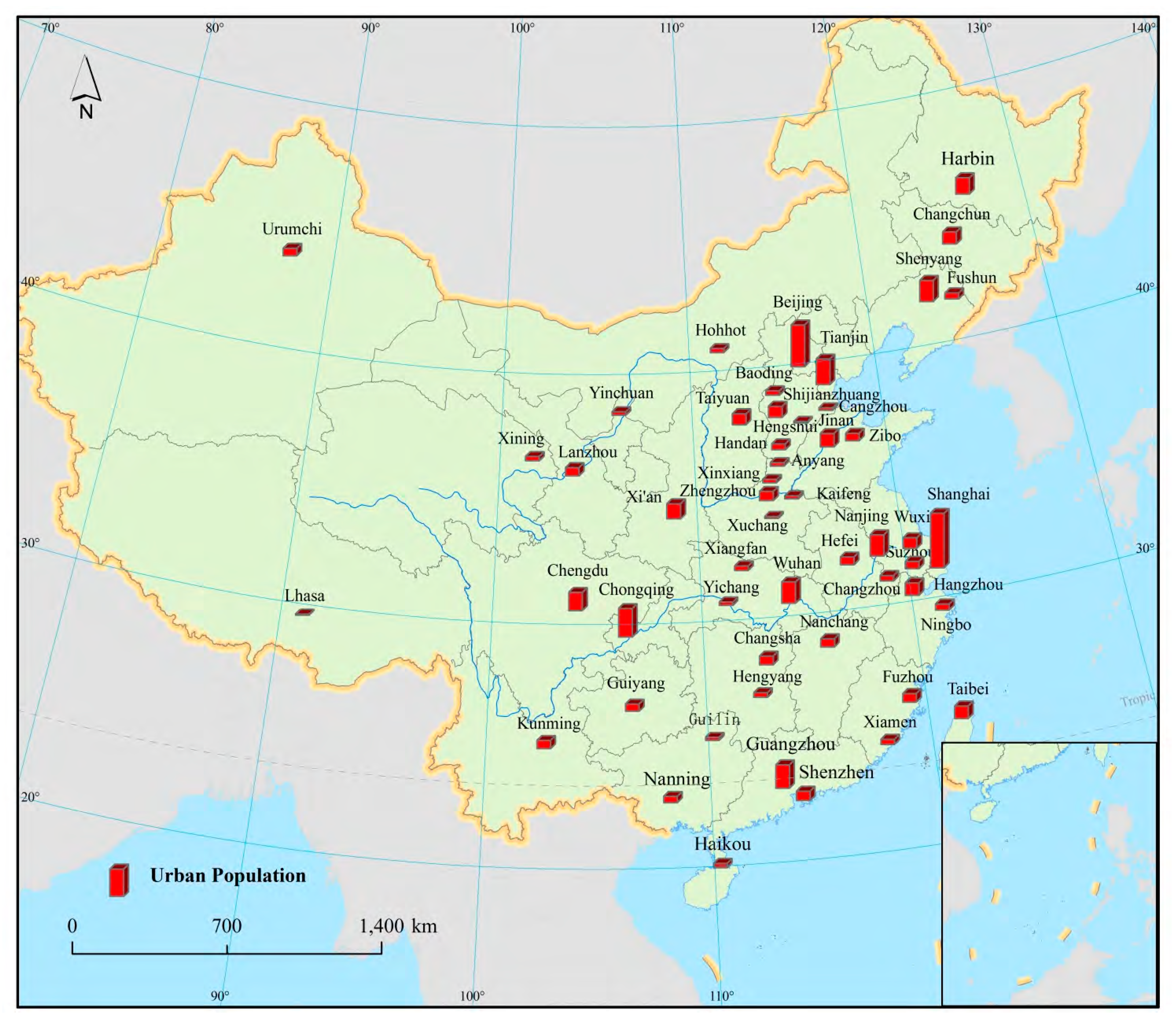
| City | Population (Thousand) | Local-Optimized Threshold | OCSVM NTL + NDVI | OCSVM NTL + LST | OCSVM NTL + NDVI + LST | |||||
|---|---|---|---|---|---|---|---|---|---|---|
| OA (%) | Kappa | OA (%) | Kappa | OA (%) | Kappa | OA (%) | Kappa | |||
| The first group: Big cities | Shanghai | 11,511.9 | 89.01 | 0.6222 | 88.16 | 0.6357 | 77.22 | 0.4623 | 87.31 | 0.6286 |
| Beijing | 8792.8 | 94.89 | 0.6521 | 94.48 | 0.6665 | 88.58 | 0.5062 | 93.94 | 0.6531 | |
| Hong Kong | 6857.1 | 79.95 | 0.5119 | 82.22 | 0.5842 | 71.31 | 0.4058 | 84.1 | 0.6106 | |
| Chongqing | 5966.9 | 87.08 | 0.6018 | 90.22 | 0.6529 | 80.59 | 0.5239 | 89.46 | 0.6469 | |
| Tianjin | 5400.2 | 90.68 | 0.5548 | 91.74 | 0.6002 | 86.69 | 0.5174 | 91.87 | 0.6176 | |
| Guangzhou | 4909.5 | 78.54 | 0.5155 | 68.94 | 0.4188 | 54.06 | 0.2345 | 65.95 | 0.3812 | |
| Nanjing | 4470.4 | 87.73 | 0.6466 | 89.17 | 0.7011 | 76.48 | 0.4891 | 88.56 | 0.6969 | |
| Wuhan | 4446.4 | 91.85 | 0.5495 | 92.15 | 0.5668 | 86.79 | 0.4642 | 91.55 | 0.5646 | |
| Shenyang | 4441.8 | 90.31 | 0.7006 | 90.56 | 0.6908 | 85.71 | 0.6314 | 90.96 | 0.7237 | |
| Chengdu | 3802.8 | 91.99 | 0.7787 | 90.63 | 0.6748 | 85.76 | 0.658 | 92.91 | 0.7682 | |
| Harbin | 3413 | 94.86 | 0.6095 | 92.52 | 0.5925 | 84.72 | 0.4095 | 91.82 | 0.5697 | |
| Xi’an | 3182 | 85.52 | 0.619 | 75.67 | 0.4947 | 55.05 | 0.2445 | 73.4 | 0.4615 | |
| Jinan | 2770.2 | 95.23 | 0.7222 | 90.74 | 0.599 | 78.92 | 0.3701 | 89.36 | 0.5619 | |
| Taipei | 2632.242 | 90.85 | 0.5528 | 90.51 | 0.6239 | 78.23 | 0.4038 | 89.16 | 0.5982 | |
| Hangzhou | 2564.2 | 86.61 | 0.5726 | 84.68 | 0.3835 | 84.32 | 0.5739 | 85.71 | 0.4558 | |
| Changchun | 2508.5 | 93.96 | 0.783 | 94.68 | 0.8154 | 90.69 | 0.7164 | 94.18 | 0.8048 | |
| Shijiazhuang | 2313.5 | 94.88 | 0.6859 | 95.12 | 0.713 | 86.87 | 0.5031 | 94.92 | 0.72 | |
| Taiyuan | 2276.9 | 89.04 | 0.564 | 89.44 | 0.5606 | 88.19 | 0.5883 | 89.44 | 0.5797 | |
| Wuxi | 2186.3 | 88.11 | 0.5963 | 86.21 | 0.5946 | 61.31 | 0.2774 | 83.4 | 0.5544 | |
| The second group:Medium cities | Shenzhen | 1968.3 | 79.04 | 0.4444 | 81.23 | 0.5768 | 69.73 | 0.3966 | 79.92 | 0.5523 |
| Zhengzhou | 1932.6 | 92.43 | 0.5903 | 92.78 | 0.6312 | 85.38 | 0.472 | 92.7 | 0.6426 | |
| Fuzhou | 1817.2 | 91.07 | 0.5376 | 90.57 | 0.457 | 91.45 | 0.584 | 91.23 | 0.5151 | |
| Changsha | 1798.9 | 92.72 | 0.7256 | 93.65 | 0.7475 | 88.68 | 0.6533 | 94.16 | 0.7758 | |
| Nanchang | 1737.5 | 87.59 | 0.6183 | 88.11 | 0.6532 | 80.73 | 0.5221 | 85.59 | 0.6035 | |
| Lanzhou | 1723.1 | 94.88 | 0.5889 | 85.93 | 0.4071 | 85.12 | 0.3912 | 85.32 | 0.3951 | |
| Kunming | 1720.7 | 93.7 | 0.6385 | 94.64 | 0.6804 | 91.25 | 0.572 | 94.35 | 0.673 | |
| Hefei | 1605.4 | 94.2 | 0.7135 | 94.97 | 0.7358 | 91.15 | 0.6403 | 94.9 | 0.7466 | |
| Urumchi | 1576.6 | 97.5 | 0.6572 | 94.65 | 0.5205 | 93.58 | 0.4735 | 94.36 | 0.5084 | |
| Zibo | 1557.4 | 91.19 | 0.3173 | 90.6 | 0.4199 | 79.94 | 0.28 | 89.48 | 0.4092 | |
| Guiyang | 1513 | 93.02 | 0.6505 | 93.75 | 0.535 | 92.69 | 0.6752 | 93.94 | 0.5994 | |
| Suzhou | 1501.4 | 88.02 | 0.5665 | 83.95 | 0.5585 | 64.15 | 0.3053 | 81.2 | 0.5207 | |
| Nanning | 1308.1 | 97.5 | 0.7443 | 98.37 | 0.8138 | 96.14 | 0.6618 | 98.18 | 0.8044 | |
| Fushun | 1260.2 | 89.15 | 0.4947 | 90.93 | 0.5456 | 84.42 | 0.4758 | 90.73 | 0.5856 | |
| Ningbo | 1257.6 | 89.76 | 0.5356 | 88.54 | 0.583 | 66.46 | 0.2804 | 85.67 | 0.5402 | |
| Handan | 1245.8 | 89.23 | 0.5867 | 90.46 | 0.6425 | 84.15 | 0.5556 | 91.69 | 0.6979 | |
| Changzhou | 1115.9 | 89.71 | 0.5398 | 88.24 | 0.5656 | 65.02 | 0.2553 | 85.35 | 0.5208 | |
| Xiamen | 1092.4 | 79.6 | 0.3562 | 81.44 | 0.4724 | 72.24 | 0.3222 | 81.17 | 0.4622 | |
| The third group: Small cities | Hengyang | 966 | 91.15 | 0.5698 | 92.8 | 0.573 | 90.74 | 0.5691 | 93.42 | 0.6331 |
| Xiangfan | 953.4 | 94.14 | 0.6961 | 94.14 | 0.6642 | 92.03 | 0.6474 | 94.41 | 0.7005 | |
| Baoding | 927.5 | 93.24 | 0.4964 | 93.38 | 0.5385 | 89.32 | 0.4671 | 93.48 | 0.5598 | |
| Xining | 909.8 | 98.99 | 0.2606 | 98.53 | 0.3442 | 98.14 | 0.3033 | 98.38 | 0.3338 | |
| Haikou | 897.7 | 84.88 | 0.4432 | 88.37 | 0.5052 | 86.21 | 0.5187 | 88.27 | 0.5168 | |
| Hohhot | 842.3 | 94.64 | 0.7457 | 77.74 | 0.4046 | 68.45 | 0.2963 | 74.64 | 0.3679 | |
| Yinchuan | 711.9 | 95.39 | 0.5424 | 94.99 | 0.5603 | 92.01 | 0.4401 | 94.3 | 0.5324 | |
| Xinxiang | 711.9 | 90.48 | 0.649 | 91.1 | 0.6999 | 69.77 | 0.3438 | 89.65 | 0.6675 | |
| Yichang | 702.2 | 96.8 | 0.5568 | 97.22 | 0.5484 | 95.75 | 0.5455 | 97.22 | 0.5813 | |
| Anyang | 688 | 87.93 | 0.6567 | 91.33 | 0.7547 | 80.5 | 0.5586 | 91.33 | 0.7594 | |
| Guilin | 629.1 | 98.47 | 0.5378 | 98.27 | 0.2551 | 98.49 | 0.5896 | 98.3 | 0.2897 | |
| Kaifeng | 592.4 | 87.2 | 0.3727 | 90.13 | 0.4768 | 85.6 | 0.4206 | 89.73 | 0.4896 | |
| Xianyang | 545.3 | 75 | 0.3226 | 78.1 | 0.4604 | 55.48 | 0.2367 | 79.52 | 0.5127 | |
| Macau | 513.4 | 59.62 | 0.1817 | 66.35 | 0.3142 | 75.96 | 0.5138 | 74.04 | 0.467 | |
| Cangzhou | 492.6 | 89.38 | 0.3986 | 91.72 | 0.5396 | 85.52 | 0.4302 | 91.59 | 0.5649 | |
| Xuchang | 401.5 | 89.18 | 0.4927 | 92.69 | 0.6573 | 81.58 | 0.4654 | 93.57 | 0.7239 | |
| Hengshui | 298.1 | 97.28 | 0.5485 | 97.5 | 0.5776 | 96.03 | 0.5578 | 97.61 | 0.6275 | |
| Lhasa | 211.4 | 96.74 | 0.6312 | 96.78 | 0.6617 | 96.34 | 0.6306 | 96.6 | 0.6489 | |
| Local-Optimized Threshold | OCSVM NTL + NDVI + LST | OCSVM NTL + NDVI | OCSVM NTL + LST | |
|---|---|---|---|---|
| Big cities | 0.7700 | 0.8190 | 0.8127 | 0.8128 |
| Medium cities | 0.9321 | 0.9175 | 0.9269 | 0.8763 |
| Small cities | 0.5439 | 0.7267 | 0.7139 | 0.6914 |
5. General Discussion
6. Conclusions
Acknowledgments
Author Contributions
Conflicts of Interest
References
- Alberti, M. The effects of urban patterns on ecosystem function. Int. Reg. Sci. Rev. 2005, 28, 168–192. [Google Scholar] [CrossRef]
- Grimmond, S.U.E. Urbanization and global environmental change: Local effects of urban warming. Geogr. J. 2007, 173, 83–88. [Google Scholar] [CrossRef]
- Johnson, M.P. Environmental impacts of urban sprawl: A survey of the literature and proposed research agenda. Environ. Plan. A 2001, 33, 717–735. [Google Scholar] [CrossRef]
- Shukla, V.; Parikh, K. The environmental consequences of urban growth: Cross national perspectives on economic development, air pollution, and city size. Urban Geogr. 1992, 13, 422–449. [Google Scholar] [CrossRef]
- Foley, J.A.; DeFries, R.; Asner, G.P.; Barford, C.; Bonan, G.; Carpenter, S.R.; Chapin, F.S.; Coe, M.T.; Daily, G.C.; Gibbs, H.K.; et al. Global consequences of land use. Science 2005, 309, 570–574. [Google Scholar]
- Kasimu, A.; Tateishi, R.; Hoan, N.T. Global urban characterization using population density, DMSP and MODIS data. In Proceedings of the Urban Remote Sensing Event, 2009 Joint, Shanghai, China, 20–22 May 2009; pp. 1–7.
- McKinney, M. Effects of urbanization on species richness: A review of plants and animals. Urban Ecosyst. 2008, 11, 161–176. [Google Scholar] [CrossRef]
- Small, C.; Pozzi, F.; Elvidge, C.D. Spatial analysis of global urban extent from DMSP-OLS night lights. Remote Sens. Environ. 2005, 96, 277–291. [Google Scholar] [CrossRef]
- Meyer, W.B.; Turner, B.L. Human population growth and global land-use/cover change. Annu. Rev. Ecol. Syst. 1992, 23, 39–61. [Google Scholar] [CrossRef]
- Ewing, R.; Rong, F. The impact of urban form on U.S. residential energy use. Hous. Policy Debate 2008, 19, 1–30. [Google Scholar] [CrossRef]
- Jensen, J.R.; Cowen, D.C. Remote sensing of urban/suburban infrastructure and socio-economic attributes. Photogram. Eng. Remote Sens. 1999, 65, 611–622. [Google Scholar]
- Tian, G.; Liu, J.; Xie, Y.; Yang, Z.; Zhuang, D.; Niu, Z. Analysis of spatio-temporal dynamic pattern and driving forces of urban land in China in 1990s using TM images and GIS. Cities 2005, 22, 400–410. [Google Scholar] [CrossRef]
- Liu, J.; Liu, M.; Zhuang, D.; Zhang, Z.; Deng, X. Study on spatial pattern of land-use change in China during 1995–2000. Sci. China Ser. D Earth Sci. 2003, 46, 373–384. [Google Scholar]
- Liu, J.; Liu, M.; Tian, H.; Zhuang, D.; Zhang, Z.; Zhang, W.; Tang, X.; Deng, X. Spatial and temporal patterns of China’s cropland during 1990–2000: An analysis based on landsat TM data. Remote Sens. Environ. 2005, 98, 442–456. [Google Scholar] [CrossRef]
- Liu, J.; Zhang, Z.; Xu, X.; Kuang, W.; Zhou, W.; Zhang, S.; Li, R.; Yan, C.; Yu, D.; Wu, S. Spatial patterns and driving forces of land use change in China during the early 21st century. J. Geogr. Sci. 2010, 20, 483–494. [Google Scholar] [CrossRef]
- Lu, D.; Tian, H.; Zhou, G.; Ge, H. Regional mapping of human settlements in southeastern China with multisensor remotely sensed data. Remote Sens. Environ. 2008, 112, 3668–3679. [Google Scholar] [CrossRef]
- Elvidge, C.; Baugh, K.; Hobson, V.; Kihn, E.; Kroehl, H.; Davis, E.; Cocero, D. Satellite inventory of human settlements using nocturnal radiation emissions: A contribution for the global toolchest. Glob. Chang. Biol. 1997, 3, 387–395. [Google Scholar] [CrossRef]
- Sudhira, H.S.; Ramachandra, T.V.; Jagadish, K.S. Urban sprawl: Metrics, dynamics and modelling using GIS. Int. J. Appl. Earth Obs. Geoinf. 2004, 5, 29–39. [Google Scholar] [CrossRef]
- Bartholomé, E.; Belward, A.S. GLC2000: A new approach to global land cover mapping from earth observation data. Int. J. Remote Sens. 2005, 26, 1959–1977. [Google Scholar] [CrossRef]
- Gamba, P.; Herold, M. Global Mapping of Human Settlement: Experiences, Datasets, and Prospects; CRC Press: Boca Raton, FL, USA, 2010. [Google Scholar]
- Schneider, A.; Friedl, M.A.; Potere, D. Mapping global urban areas using MODIS 500 m data: New methods and datasets based on “urban ecoregions”. Remote Sens. Environ. 2010, 114, 1733–1746. [Google Scholar] [CrossRef]
- Zhang, Q.; Seto, K.C. Mapping urbanization dynamics at regional and global scales using multi-temporal DMSP/OLS nighttime light data. Remote Sens. Environ. 2011, 115, 2320–2329. [Google Scholar] [CrossRef]
- Arino, O.; Gross, D.; Ranera, F.; Bourg, L.; Bicheron, P.; Latham, J.; di Gregorio, A.; Brockman, C.; Leroy, M.; Witt, R.; et al. Globcover: ESA Service for global land cover from MERIS. In Proceedings of the IEEE International Geoscience and Remote Sensing Symposium, Barcelona, Spain, 23–28 July 2007; pp. 2412–2415.
- Imhoff, M.L.; Lawrence, W.T.; Stutzer, D.C.; Elvidge, C.D. A technique for using composite DMSP/OLS “city lights” satellite data to map urban area. Remote Sens. Environ. 1997, 61, 361–370. [Google Scholar] [CrossRef]
- Elvidge, C.D.; Sutton, P.C.; Tuttle, B.T.; Ghosh, T.; Baugh, K.E. Global urban mapping based on nighttime lights. In Global Mapping of Human Settlement; CRC Press: Boca Raton, FL, USA, 2009. [Google Scholar]
- Milesi, C.; Elvidge, C.D.; Nemani, R.R.; Running, S.W. Assessing the environmental impacts of human settlements using satellite data. Manag. Environ. Qual. 2003, 14, 99–107. [Google Scholar] [CrossRef]
- Elvidge, C.D.; Baugh, K.E.; Dietz, J.B.; Bland, T.; Sutton, P.C.; Kroehl, H.W. Radiance calibration of DMSP-OLS low-light imaging data of human settlements. Remote Sens. Environ. 1999, 68, 77–88. [Google Scholar] [CrossRef]
- Elvidge, C.D.; Imhoff, M.L.; Baugh, K.E.; Hobson, V.R.; Nelson, I.; Safran, J.; Dietz, J.B.; Tuttle, B.T. Night-time lights of the world: 1994–1995. ISPRS J. Photogramm. Remote Sens. 2001, 56, 81–99. [Google Scholar] [CrossRef]
- Henderson, M.; Yeh, E.T.; Gong, P.; Elvidge, C.; Baugh, K. Validation of urban boundaries derived from global night-time satellite imagery. Int. J. Remote Sens. 2003, 24, 595–609. [Google Scholar] [CrossRef]
- Sutton, P.C. A scale-adjusted measure of “urban sprawl” using nighttime satellite imagery. Remote Sens. Environ. 2003, 86, 353–369. [Google Scholar] [CrossRef]
- Amaral, S.; Câmara, G.; Monteiro, A.M.V.; Quintanilha, J.A.; Elvidge, C.D. Estimating population and energy consumption in Brazilian Amazonia using DMSP night-time satellite data. Comput. Environ. Urban Syst. 2005, 29, 179–195. [Google Scholar] [CrossRef]
- Elvidge, C.D.; Cinzano, P.; Pettit, D.R.; Arvesen, J.; Sutton, P.; Small, C.; Nemani, R.; Longcore, T.; Rich, C.; Safran, J.; et al. The nightsat mission concept. Int. J. Remote Sens. 2007, 28, 2645–2670. [Google Scholar] [CrossRef]
- Owen, T.W. Using DMSP-OLS light frequency data to categorize urban environments associated with US climate observing stations. Int. J. Remote Sens. 1998, 19, 3451–3456. [Google Scholar] [CrossRef]
- Sutton, P.; Roberts, D.; Elvidge, C.; Baugh, K. Census from heaven: An estimate of the global human population using night-time satellite imagery. Int. J. Remote Sens. 2001, 22, 3061–3076. [Google Scholar] [CrossRef]
- Cao, X.; Chen, J.; Imura, H.; Higashi, O. A SVM-based method to extract urban areas from DMSP-OLS and SPOT VGT data. Remote Sens. Environ. 2009, 113, 2205–2209. [Google Scholar] [CrossRef]
- Pandey, B.; Joshi, P.K.; Seto, K.C. Monitoring urbanization dynamics in India using DMSP/OLS night time lights and SPOT-VGT data. Int. J. Appl. Earth Obs. Geoinf. 2013, 23, 49–61. [Google Scholar] [CrossRef]
- Yang, Y.; He, C.; Zhang, Q.; Han, L.; Du, S. Timely and accurate national-scale mapping of urban land in China using defense meteorological satellite program’s operational linescan system nighttime stable light data. J. Appl. Remote Sens. 2013, 7, 073535. [Google Scholar] [CrossRef]
- Zhou, Y.; Smith, S.J.; Elvidge, C.D.; Zhao, K.; Thomson, A.; Imhoff, M. A cluster-based method to map urban area from DMSP/OLS nightlights. Remote Sens. Environ. 2014, 147, 173–185. [Google Scholar] [CrossRef]
- Gallo, K.P.; Tarpley, J.D.; McNab, A.L.; Karl, T.R. Assessment of urban heat islands: A satellite perspective. Atmos. Res. 1995, 37, 37–43. [Google Scholar] [CrossRef]
- Rotem-Mindali, O.; Michael, Y.; Helman, D.; Lensky, I.M. The role of local land-use on the urban heat island effect of Tel AVIV as assessed from satellite remote sensing. Appl. Geogr. 2015, 56, 145–153. [Google Scholar] [CrossRef]
- Dewan, A.M.; Corner, R.J. Impact of land use and land cover changes on urban land surface temperature. In Dhaka Megacity; Springer: Berlin, Germany, 2014; pp. 219–238. [Google Scholar]
- Gallo, K.P.; McNab, A.L.; Karl, T.R.; Brown, J.F.; Hood, J.J.; Tarpley, J.D. The use of NOAA AVHRR data for assessment of the urban heat island effect. J. Appl. Meteorol. 1993, 32, 899–908. [Google Scholar] [CrossRef]
- Lu, D.; Weng, Q. Use of impervious surface in urban land-use classification. Remote Sens. Environ. 2006, 102, 146–160. [Google Scholar] [CrossRef]
- Yang, F.; Matsushita, B.; Yang, W.; Fukushima, T. Mapping the human footprint from satellite measurements in Japan. ISPRS J. Photogramm. Remote Sens. 2014, 88, 80–90. [Google Scholar] [CrossRef] [Green Version]
- Melesse, A.M.; Graham, W.D.; Jordan, J.D. Spatially distributed watershed mapping and modeling: Thermal maps and vegetation indices to enhance land cover and surface microclimate mapping (part 1). J. Spat. Hydrol. 2003, 3, 1–29. [Google Scholar]
- Julien, Y.; Sobrino, J.A.; Jiménez-Muñoz, J.C. Land use classification from multitemporal landsat imagery using the yearly land cover dynamics (YLCD) method. Int. J. Appl. Earth Obs. Geoinf. 2011, 13, 711–720. [Google Scholar] [CrossRef]
- Sobrino, J.; Raissouni, N.; Lobo, A. Monitoring the Iberian peninsula land cover using NOAA-AVHRR data. Phys. Meas. Signat. Remote Sens. 1997, 787–794. [Google Scholar]
- Lambin, E.; Ehrlich, D. Combining vegetation indices and surface temperature for land-cover mapping at broad spatial scales. Remote Sens. 1995, 16, 573–579. [Google Scholar] [CrossRef]
- Lambin, E.; Ehrlich, D. The surface temperature-vegetation index space for land cover and land-cover change analysis. Int. J. Remote Sens. 1996, 17, 463–487. [Google Scholar] [CrossRef]
- Hao, R.; Yu, D.; Sun, Y.; Cao, Q.; Liu, Y.; Liu, Y. Integrating multiple source data to enhance variation and weaken the blooming effect of DMSP-OLS light. Remote Sens. 2015, 7, 1422–1440. [Google Scholar] [CrossRef]
- Schölkopf, B.; Platt, J.C.; Shawe-Taylor, J.; Smola, A.J.; Williamson, R.C. Estimating the support of a high-dimensional distribution. Neural Comput. 2001, 13, 1443–1471. [Google Scholar] [CrossRef] [PubMed]
- Tax, D.M.J. One-Class Classification; Delft University of Technology: Delft, The Netherlands, 2001. [Google Scholar]
- Sanchez-Hernandez, C.; Boyd, D.S.; Foody, G.M. One-class classification for mapping a specific land-cover class: SVDD classification of fenland. IEEE Trans. Geosci. Remote Sens. 2007, 45, 1061–1073. [Google Scholar] [CrossRef]
- Munoz-Mari, J.; Bruzzone, L.; Camps-Valls, G. A support vector domain description approach to supervised classification of remote sensing images. IEEE Trans. Geosci. Remote Sens. 2007, 45, 2683–2692. [Google Scholar] [CrossRef]
- Li, P.; Xu, H. Land-cover change detection using one-class support vector machine. Photogramm. Eng. Remote Sens. 2010, 76, 255–263. [Google Scholar] [CrossRef]
- Guo, Q.; Kelly, M.; Graham, C.H. Support vector machines for predicting distribution of sudden Oak death in California. Ecol. Model. 2005, 182, 75–90. [Google Scholar] [CrossRef]
- Liu, Z.; He, C.; Zhang, Q.; Huang, Q.; Yang, Y. Extracting the dynamics of urban expansion in China using DMSP-OLS nighttime light data from 1992 to 2008. Lands. Urban Plan. 2012, 106, 62–72. [Google Scholar] [CrossRef]
- Deng, X.; Huang, J.; Rozelle, S.; Uchida, E. Growth, population and industrialization, and urban land expansion of China. J. Urban Econ. 2008, 63, 96–115. [Google Scholar] [CrossRef]
- National Bureau of Statistics of China. China Statistical Yearbook 1991; China Statistics Press: Beijing, China, 1991.
- National Bureau of Statistics of China. China Statistical Yearbook 2013; China Statistics Press: Beijing, China, 2013.
- Song, Y.; Ding, C. Urbanization in China: Critical Issues in An Era of Rapid Growth; Lincoln Institute of Land Policy: Cambridge, MA, USA, 2007. [Google Scholar]
- Maimaitiming, A.; Xiaolei, Z.; Huhua, C. Urbanization in western China. Chin. J. Popul. Res. Environ. 2013, 11, 79–86. [Google Scholar] [CrossRef]
- Gu, J.; Li, X.; Huang, C.; Okin, G.S. A simplified data assimilation method for reconstructing time-series MODIS NDVI data. Adv. Space Res. 2009, 44, 501–509. [Google Scholar] [CrossRef]
- Huete, A.; Didan, K.; Miura, T.; Rodriguez, E.P.; Gao, X.; Ferreira, L.G. Overview of the radiometric and biophysical performance of the MODIS vegetation indices. Remote Sens. Environ. 2002, 83, 195–213. [Google Scholar] [CrossRef]
- Hulley, G.C.; Hook, S.J. Intercomparison of versions 4, 4.1 and 5 of the MODIS land surface temperature and emissivity products and validation with laboratory measurements of sand samples from the Namib desert, Namibia. Remote Sens. Environ. 2009, 113, 1313–1318. [Google Scholar]
- Holben, B.N. Characteristics of maximum-value composite images from temporal AVHRR data. Int. J. Remote Sens. 1986, 7, 1417–1434. [Google Scholar] [CrossRef]
- Peng, S.; Piao, S.; Ciais, P.; Friedlingstein, P.; Ottle, C.; Breon, F.M.; Nan, H.; Zhou, L.; Myneni, R.B. Surface urban heat island across 419 global big cities. Environ. Sci. Technol. 2012, 46, 696–703. [Google Scholar] [CrossRef] [PubMed]
- Zhao, L.; Lee, X.; Smith, R.B.; Oleson, K. Strong contributions of local background climate to urban heat islands. Nature 2014, 511, 216–219. [Google Scholar] [CrossRef] [PubMed]
- National Bureau of Statistics of China. China Statistical Yearbook 2007; China Statistics Press: Beijing, China, 2007.
- Zhang, Q.; Schaaf, C.; Seto, K.C. The vegetation adjusted ntl urban index: A new approach to reduce saturation and increase variation in nighttime luminosity. Remote Sens. Environ. 2013, 129, 32–41. [Google Scholar] [CrossRef]
- Weng, Q. Thermal infrared remote sensing for urban climate and environmental studies: Methods, applications, and trends. ISPRS J. Photogramm. Remote Sens. 2009, 64, 335–344. [Google Scholar] [CrossRef]
- Gallo, K.P.; McNab, A.L.; Karl, T.R.; Brown, J.F.; Hood, J.J.; Tarpley, J.D. The use of a vegetation index for assessment of the urban heat island effect. Int. J. Remote Sens. 1993, 14, 2223–2230. [Google Scholar] [CrossRef]
- Landsberg, H.E. The Urban Climate; Academic Press: New York, NY, USA, 1981; Volume 28. [Google Scholar]
- He, C.; Shi, P.; Li, J.; Chen, J.; Pan, Y.; Li, J.; Zhuo, L.; Ichinose, T. Restoring urbanization process in China in the 1990s by using non-radiance-calibrated DMSP/OLS nighttime light imagery and statistical data. Chin. Sci. Bull. 2006, 51, 1614–1620. [Google Scholar] [CrossRef]
- Huang, C.; Davis, L.; Townshend, J. An assessment of support vector machines for land cover classification. Int. J. Remote Sens. 2002, 23, 725–749. [Google Scholar] [CrossRef]
- Congalton, R.G.; Green, K. Assessing the accuracy of remotely sensed data: Principles and practices, second edition. CRC Press: Boca Raton, FL, USA, 2008. [Google Scholar]
- Pontius, R.G., Jr.; Millones, M. Death to kappa: Birth of quantity disagreement and allocation disagreement for accuracy assessment. Int. J. Remote Sens. 2011, 32, 4407–4429. [Google Scholar] [CrossRef]
- Foody, G.M. Status of land cover classification accuracy assessment. Remote Sens. Environ. 2002, 80, 185–201. [Google Scholar] [CrossRef]
- Neubert, M.; Meinel, G. Evaluation of segmentation programs for high resolution remote sensing applications. In Proceedings of the International ISPRS Workshop “High Resolution Mapping from Space”, Hannover, Germany, 6–8 October 2003.
© 2015 by the authors; licensee MDPI, Basel, Switzerland. This article is an open access article distributed under the terms and conditions of the Creative Commons Attribution license (http://creativecommons.org/licenses/by/4.0/).
Share and Cite
Zhang, X.; Li, P.; Cai, C. Regional Urban Extent Extraction Using Multi-Sensor Data and One-Class Classification. Remote Sens. 2015, 7, 7671-7694. https://doi.org/10.3390/rs70607671
Zhang X, Li P, Cai C. Regional Urban Extent Extraction Using Multi-Sensor Data and One-Class Classification. Remote Sensing. 2015; 7(6):7671-7694. https://doi.org/10.3390/rs70607671
Chicago/Turabian StyleZhang, Xiya, Peijun Li, and Cai Cai. 2015. "Regional Urban Extent Extraction Using Multi-Sensor Data and One-Class Classification" Remote Sensing 7, no. 6: 7671-7694. https://doi.org/10.3390/rs70607671