Empirical Results of a Surface-Level GNSS-R Experiment in a Wave Channel

Abstract

The scattering of GNSS signals over a water surface is studied when the receiver is at a low height, as in GNSS-R coastal altimetry. The precise determination of the local sea level and wave state from the coast will provide useful altimetry and wave information as “dry” tide and wave gauges. An experiment has been conducted at the Canal d'Investigació i Experimentació Marítima (CIEM) wave channel for two simulated “sea” states. The GNSS-reflectometer used is the P(Y) and C/A ReflectOmeter (PYCARO) instrument, a closed-loop receiver with delay and Doppler tracking loops that uses the conventional GNSS-R technique for the GPS C/A code. After retracking of the scattered GPS signals, the coherent and incoherent components have been studied. To reproduce the transmitted GPS signals indoors, a Rohde and Schwarz signal generator is used. It is found that, despite the ratio of the coherent and incoherent components being ~1, the coherent component is strong enough that it can be tracked. The coherent component comes from clusters of points on the surface that approximately satisfy the specular reflection conditions (“roughed facet”). The Pearson’s linear correlation coefficients of the derived “sea” surface height with the wave gauge data are: 0.78, 0.85 and 0.81 for a SWH = 36 cm and 0.34, 0.74, and 0.72 for a SWH = 64 cm, respectively, for transmitter elevation angles of ${\text{θ}}_{\text{e}}$ = 60°, 75° and 86°, respectively. Finally, the rms phase of the received signal before the retracking processing is used to estimate the effective rms surface height of the ‘facets’, where the waves get scattered. It is found to be between 2.5- and 4.1-times smaller than the theoretical values corresponding to the half of the coherent reflectivity decaying factor.

1. Introduction

GNSS (Global Navigation Satellite System) Earth-reflected signals can be used as sources of opportunity for mesoscale ocean altimetry with improved temporal resolution as compared to traditional monostatic radar altimetry [1]. This relatively novel technology is known as GNSS reflectometry (GNSS-R). The first experimental evidence of GPS reflected signals dates back to 1994 [2], and it was stated that, since the Rayleigh criterion was not satisfied, the scattering was diffuse. In 1996, Garrison et al. [3] performed three different aircraft experiments over the ocean using a GPS receiver. Results showed that a specialized receiver must be developed to collect the Earth-reflected signals over a rough surface, because the scattering process distorts the signal, and the receiver lost tracking. In 2000, Zavorotny and Voronovich [4] developed a bistatic model of the ocean scattered GPS signals providing an analytical expression of the “waveforms” under the Kirchhoff approximation. Assuming that coherent scattering is negligible, the bistatic scattering coefficient was derived under the geometric optics limit, for a sea surface model with Gaussian distribution of the slopes, and a final expression of the “waveform” was derived. During the last decade, additional experimental [5,6,7,8] and theoretical [9,10,11,12] works have been performed to investigate the feasibility of this bistatic radar system to perform accurate ocean altimetry, usually with open-loop receivers, and using a model of the scattering geometry to center the delay and Doppler tracking windows.

In this experiment, the P(Y) and C/A ReflectOmeter (PYCARO) (due to the limitations of the instrumentation, only synthetic GPS L1 C/A signals could be generated for this indoor experiment; note that the GPS P(Y) code is encrypted and is not publicly available) is used. PYCARO is a closed-loop GNSS-R receiver with delay and Doppler tracking loops [13,14] that uses conventional GNSS-R (cGNSS-R) for the open GPS codes (C/A) and reconstructed GNSS-R (rGNSS-R) for the encrypted ones. The coherent component of the scattered signals is studied experimentally in the Canal d'Investigació i Experimentació Marítima (CIEM)/UPC-BarcelonaTech wave channel [15]. The results of this experiment can be of interest in GNSS-R waves and coastal altimetry studies, because of the low-altitude of the receiver over the surface and its static position. The monitoring of the local sea level has an increasing interest for society, because it is an indicator of global climate change [16]. In order to use space-borne altimeter data to compute the mean sea level variations over time, there is a need to account for biases and drifts in the instruments [17].

Section 2 describes the experimental setup and the ground truth data generated during the experimental campaign. Section 3.1 studies the number of specular points inside the scattering area. Section 3.2 evaluates the performance for coastal applications. Section 3.3 analyzes the ratio of the coherent-to-incoherent components as observed by the PYCARO instrument. In Section 3.4, the GPS signals before retracking are used to infer the rms surface height of the small-scale waves as observed by PYCARO. This is used to properly account for the coherent scattering over the small-scale 1D mechanically-driven waves. Finally, Section 4 summarizes the main results of this study.

2. Experiment Description

2.1. Experimental Setup

Coherent GNSS reflected signals have been tracked and reported in the past [18,19,20,21]. In 2012, the PYCARO GNSS-R instrument flying along the Catalan coast tracked the coherent reflected GPS signals under moderate-to-high wind conditions (>11 m/s), and high elevation angles (${\text{θ}}_{\text{e}}$ > 30°) [13]. That evidence triggered the need to better understand the scattering mechanisms, and to that end, an experiment was performed during April 2013 in the CIEM (Figure 1), at the premises of the Civil Engineering School of the Universitat Politècnica de Catalunya-BarcelonaTech.

Figure 1. View of the Canal d'Investigació i Experimentació Marítima (CIEM) wave channel at the Laboratori d’Enginyeria Marítima (Universitat Politècnica de Catalunya). Wave channel dimensions are: width = 3 m, length = 100 m and depth = 5 m.

Figure 1. View of the Canal d'Investigació i Experimentació Marítima (CIEM) wave channel at the Laboratori d’Enginyeria Marítima (Universitat Politècnica de Catalunya). Wave channel dimensions are: width = 3 m, length = 100 m and depth = 5 m.

Since this is an indoor facility, a Rohde and Schwarz SMU 200 A vector signal generator (Figure 2 on the left) was used to synthesize controlled GPS L1 C/A signals [22]. One single PRN code was emitted at a time. Synthetic GPS signals were emitted using a 15-dB gain GPS right-hand circular polarized antenna (RHCP) array. The reflected signals were collected by a twin GPS antenna array with left-hand circular polarization (LHCP). The PYCARO GNSS-R instrument processed the data, and it was connected to a laptop for monitoring the instrument’s parameters and to log the data. Both antennas were placed over the channel at static locations over two movable bridges (the antenna far field is at 1.6 m of the antenna, and the distance of the antenna over the water surface is larger than 3 m) (Figure 2) at a height of ~3 m above the water (Table 1). The height of the antennas varied a few centimeters because the inclination of their ground plane over the surface was adjusted as a function of the selected elevation angle. The separation of the bridges was adjustable, so that the antenna footprints over the water surface overlapped for all elevation angles (GNSS satellites can be observed for much lower elevation angles. During this experiment, only a limited number of days was available in the CIEM wave channel to perform the experiment. The authors decided to select elevation angles larger than 45°, because this is the operational range of future missions.) (${\text{θ}}_{\text{e}}$= 45°, 60°, 75°, 86°) (The antennas could not be closer than the size of the ground planes, so that the maximum elevation angle was actually 86°, and not 90°). The emitted GPS L1 C/A signal was calibrated to receive the same power level (direct signal) as in a real scenario ${\text{P}}_{\text{R}}$ ~ −130 dBm [23] (p. 75). Two datasets of 30 min each were collected in the CIEM wave channel in which 1D mechanically-driven waves were created with a significant wave height of 36 cm and 64 cm (Figure 3).

Figure 2. View of the experiment set-up: SMU 200 A vector signal generator, P(Y) and C/A ReflectOmeter (PYCARO) instrument and the two 15-dB gain antenna arrays.

Figure 2. View of the experiment set-up: SMU 200 A vector signal generator, P(Y) and C/A ReflectOmeter (PYCARO) instrument and the two 15-dB gain antenna arrays.

Table 1. Height of the antenna over the surface, sizes of the footprint, the first Fresnel zone and the scattering cells and cutoff wavenumbers as a function of the elevation angle. The antenna footprint is obtained as the intersection at different angles (elevation angles) of a plane (water surface mean) with the antenna radiation pattern. The scattering cell is obtained as the area on the water surface that allows scattering forward the GPS signals through the receiver antenna, taking into account the slopes of the waves and the surface roughness.

${\text{θ}}_e$ (Degrees)	45°	60°	75°	86°
Height (m), $\text{H}$	3.44	3.37	3.28	3.20
Main axis antenna footprint (m)	4.92	4	3.46	2.32
Major axis first Fresnel zone (m) ${\text{r}}_{\text{b}}=\sqrt{\raisebox{1ex}{$\text{λH}$}\!\left/ \!\raisebox{-1ex}{${\text{sinθ}}_{\text{e}}$}\right.+{\left(\raisebox{1ex}{$\text{λ}$}\!\left/ \!\raisebox{-1ex}{$2{\text{sinθ}}_{\text{e}}$}\right.\right)}^2}$	1.94	1.73	1.62	1.57
Minor axis first Fresnel zone (m) ${\text{r}}_{\text{a}}={\text{r}}_{\text{b}}{\text{sinθ}}_{\text{e}}$	1.37	1.49	1.56	1.56
Main axis scattering cell (m) SWH = 36 cm, ${\text{L}}_{\text{scatt}}$	0.34	0.26	0.22	0.22
Main axis scattering cell (m) SWH = 64 cm, ${\text{L}}_{\text{scatt}}$	1.36	1.08	0.94	0.90
Cutoff wavenumber (rad/m) SWH = 36 cm, ${\text{N}}_{\text{cutoff}}=\raisebox{1ex}{$2\text{π}$}\!\left/ \!\raisebox{-1ex}{${\text{L}}_{\text{scatt}}$}\right.$	18.48	24.16	28.56	28.56
Cutoff wavenumber (rad/m) SWH = 64 cm, ${\text{N}}_{\text{cutoff}}=\raisebox{1ex}{$2\text{π}$}\!\left/ \!\raisebox{-1ex}{${\text{L}}_{\text{scatt}}$}\right.$	4.62	5.81	6.68	6.98

Table 1. Height of the antenna over the surface, sizes of the footprint, the first Fresnel zone and the scattering cells and cutoff wavenumbers as a function of the elevation angle. The antenna footprint is obtained as the intersection at different angles (elevation angles) of a plane (water surface mean) with the antenna radiation pattern. The scattering cell is obtained as the area on the water surface that allows scattering forward the GPS signals through the receiver antenna, taking into account the slopes of the waves and the surface roughness.

${\text{θ}}_e$ (Degrees)	45°	60°	75°	86°
Height (m), $\text{H}$	3.44	3.37	3.28	3.20
Main axis antenna footprint (m)	4.92	4	3.46	2.32
Major axis first Fresnel zone (m) ${\text{r}}_{\text{b}}=\sqrt{\raisebox{1ex}{$\text{λH}$}\!\left/ \!\raisebox{-1ex}{${\text{sinθ}}_{\text{e}}$}\right.+{\left(\raisebox{1ex}{$\text{λ}$}\!\left/ \!\raisebox{-1ex}{$2{\text{sinθ}}_{\text{e}}$}\right.\right)}^2}$	1.94	1.73	1.62	1.57
Minor axis first Fresnel zone (m) ${\text{r}}_{\text{a}}={\text{r}}_{\text{b}}{\text{sinθ}}_{\text{e}}$	1.37	1.49	1.56	1.56
Main axis scattering cell (m) SWH = 36 cm, ${\text{L}}_{\text{scatt}}$	0.34	0.26	0.22	0.22
Main axis scattering cell (m) SWH = 64 cm, ${\text{L}}_{\text{scatt}}$	1.36	1.08	0.94	0.90
Cutoff wavenumber (rad/m) SWH = 36 cm, ${\text{N}}_{\text{cutoff}}=\raisebox{1ex}{$2\text{π}$}\!\left/ \!\raisebox{-1ex}{${\text{L}}_{\text{scatt}}$}\right.$	18.48	24.16	28.56	28.56
Cutoff wavenumber (rad/m) SWH = 64 cm, ${\text{N}}_{\text{cutoff}}=\raisebox{1ex}{$2\text{π}$}\!\left/ \!\raisebox{-1ex}{${\text{L}}_{\text{scatt}}$}\right.$	4.62	5.81	6.68	6.98

Figure 3. View of the HR Wallingford Wave Probe Monitor used as a reference system during the experiment (encircled on the left-hand side).

Figure 3. View of the HR Wallingford Wave Probe Monitor used as a reference system during the experiment (encircled on the left-hand side).

2.2. Scenario and Ground Truth Data

Ground truth data were recorded during the experiment. An HR Wallingford wave probe monitor [24] located exactly in the center of the transmitter and receiver was used as a reference system to measure the time-evolution of the water level. The Pearson’s linear correlation factors of the waves heights vs. the celerities and the periods are respectively 0.61 (Figure 4a) and 0.53 (Figure 4c) for a SWH = 36 cm and 0.52 (Figure 4b) and 0.42 (Figure 4d) for a SWH = 64 cm. The wave’s slope distributions are well fitted by Rayleigh pdfs (Figure 4e,f). The slopes were computed as the ratio of the height over the wavelength of individual waves from the wave probe data. At a speed of the waves of 1.6 m/s (Figure 4a,b) and with a period of the waves of 2.5 s (Figure 4c,d), the wavelength is around 4 m. This means that during the coherent integration time ${\text{T}}_{\text{c}}$ = 20 ms, the wave height difference inside the antenna footprint (Table 1) was as high as ~30 cm for a SWH = 64 cm (Figure 4b). During the coherent integration time, the roughness inside the first Fresnel zone (Table 1) included wave heights as high as ~10 cm for celerities and wave periods lower than ~1.3 m/s and ~1.3 s, respectively (Figure 4b,d). During this time period, the surface was practically frozen (the wave with a phase velocity of 1.6 m/s will move horizontally by 3 cm), so that the signal was coherent temporally. As will be shown later (Section 3), scattered waves collected by the receiver antenna get “reflected” in clustered regions, almost “facets” where a quasi-specular reflection takes place (Figure 5). It could be stated that a “relaxed” specular reflection is taking place, with the scattering process taking place in many points around the nominal specular reflection point. A “relaxed” Rayleigh criterion is introduced to account for the small-scale roughness of the surface with respect to the facet where the specular reflection is taking place. This is not satisfied during these periods, which account for wavenumbers higher than the cutoff wavenumber (Table 1). During the experiment, PYCARO tracked the coherent component of the scattered field during large portions of the dataset. In Section 3.3, the total scattered field is re-constructed to generate the scattered field by the complete footprint.

Figure 4. (a) Correlation celerity vs. wave height for a SWH = 36 cm; (b) correlation celerity vs. wave height for a SWH = 64 cm; (c) correlation period vs. wave height for a SWH = 36 cm; (d) correlation period vs. wave height for a SWH = 64 cm; (e) slope distribution for a SWH = 36 cm; (f) slope distribution for a SWH = 64 cm.

Figure 4. (a) Correlation celerity vs. wave height for a SWH = 36 cm; (b) correlation celerity vs. wave height for a SWH = 64 cm; (c) correlation period vs. wave height for a SWH = 36 cm; (d) correlation period vs. wave height for a SWH = 64 cm; (e) slope distribution for a SWH = 36 cm; (f) slope distribution for a SWH = 64 cm.

3. Experimental Results: Methodology and Discussion

3.1. Number of Specular Points inside the Scattering Area

The forward-scattering mechanisms of the GPS signals over the sea surface are still a matter of investigation. Despite many models having been studied, including the small slope approximation (SSA) model [25] and the two-scale composite model (TSM) [26], in the case of the GNSS-R, the geometrics optics limit of the Kirchhoff model (KGO) is the one most widely used [4,8,27,28] because of its simplicity and its capability to reproduce the cross-polar experimental data in the forward direction. The scattering of electromagnetic waves from the sea is strongly affected by its roughness, being the total scattered field the combination of many electromagnetic waves coming from multiple individual scatterers on the surface. In this situation, quasi-specular reflections dominate, since, according to the TSM, this type of scattering is produced mostly by the large-scale components of the surface.

This experiment focus on the evaluation of the scattering due to the small scale (roughness scales with associated wavenumbers higher than the cutoff wavenumber (Table 1)) of the water surface. To analyze the results obtained in this experiment, the shape of the water height is studied to assess the occurrence of specular points. The water surface is partitioned into 90,000 smaller surface patches equal to the number of coherent integration times (${\text{T}}_{\text{c}}$ = 20 ms) during each dataset (the length of each dataset is 30 min). The scattering field during each shot is given by [29]:

$${\text{E}}_{\text{n}}\left(\text{t}\right)=\text{W}\left({\text{ρ}}_{\text{n}},\text{t}\right){\displaystyle \sum }_{\text{i}=1}^{{\text{N}}_{\text{n}}\left(\text{t}\right)}{\text{A}}_{{\text{n}}_{\text{i}}}\left(\text{t}\right){\text{e}}^{\text{j}{\text{ϕ}}_{{\text{n}}_{\text{i}}}\left(\text{t}\right)}$$

(1)

where $\text{t}$ is the time, ${\text{N}}_{\text{n}}$ is the number of specular points around the nominal one, ${\text{ A}}_{{\text{n}}_{\text{i}}}$ is the amplitude (ruled by the local curvature of the water surface in the specular point [29]), $\text{j =}\sqrt{\text{-1}}$is the imaginary unit and ${\text{ϕ}}_{{\text{n}}_{\text{i}}}$ is the phase defined as [29]:

$${\text{ϕ}}_{{\text{n}}_{\text{i}}}=\text{j}\left({\text{θ}}_{\text{i}}-2{\text{πF}}_{\text{i}}\text{t}+{\text{kX}}_{\text{i}}\right)$$

(2)

where ${\text{θ}}_{\text{i}}$ is the angular speed of the carrier, ${\text{F}}_{\text{i}}$ is the Doppler shift of the i-th specular point, $\text{k}$ is the carrier wavenumber and ${\text{X}}_{\text{i}}$ is the range between the i-th specular point and the scattering cell center. ${\text{ϕ}}_{{\text{n}}_{\text{i}}}$ is related to the ranges from the transmitter to the i-th specular point and from it to the receiver through the variable ${\text{X}}_{\text{i}}$. Finally, $\text{W}\left({\text{ρ}}_{\text{n}},\text{t}\right)$ is a deterministic, range-dependent term defined in [29] with ${\text{ρ}}_{\text{n}}$ being the projection in the horizontal plane of the positioning vector of the scattering cell center.

For specular points inside a scattering cell, $\text{W}$ can be assumed to be constant and equal to the corresponding value at the center of the scattering cell. The variations in the signals phase due to the variations in Doppler and position of the specular points around the nominal one can be modelled as a stochastic process [29].

The scattered field in the specular direction is composed of a coherent component and a random Hoyt-distributed incoherent component [30] (p. 126). The first one comes from the coherent combination of the scattering on the individual facets within the first Fresnel zone. The incoherent component is the result of the random combination of electromagnetic waves coming from other scatterers within the glistening zone that add together at the receiving antenna. It is also shown [30] (p. 150) that in directions different from the specular one, the scattering is always incoherent.

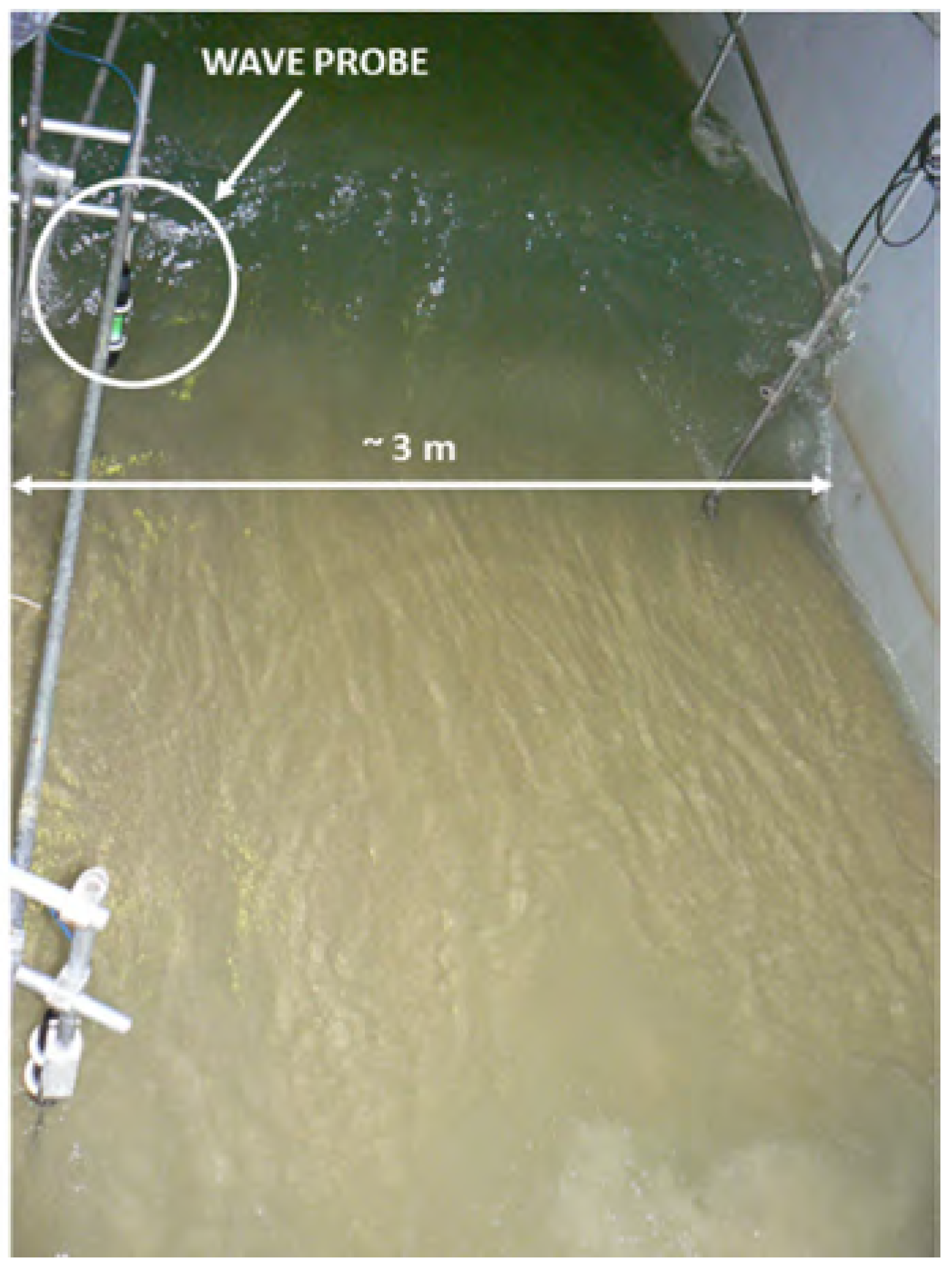
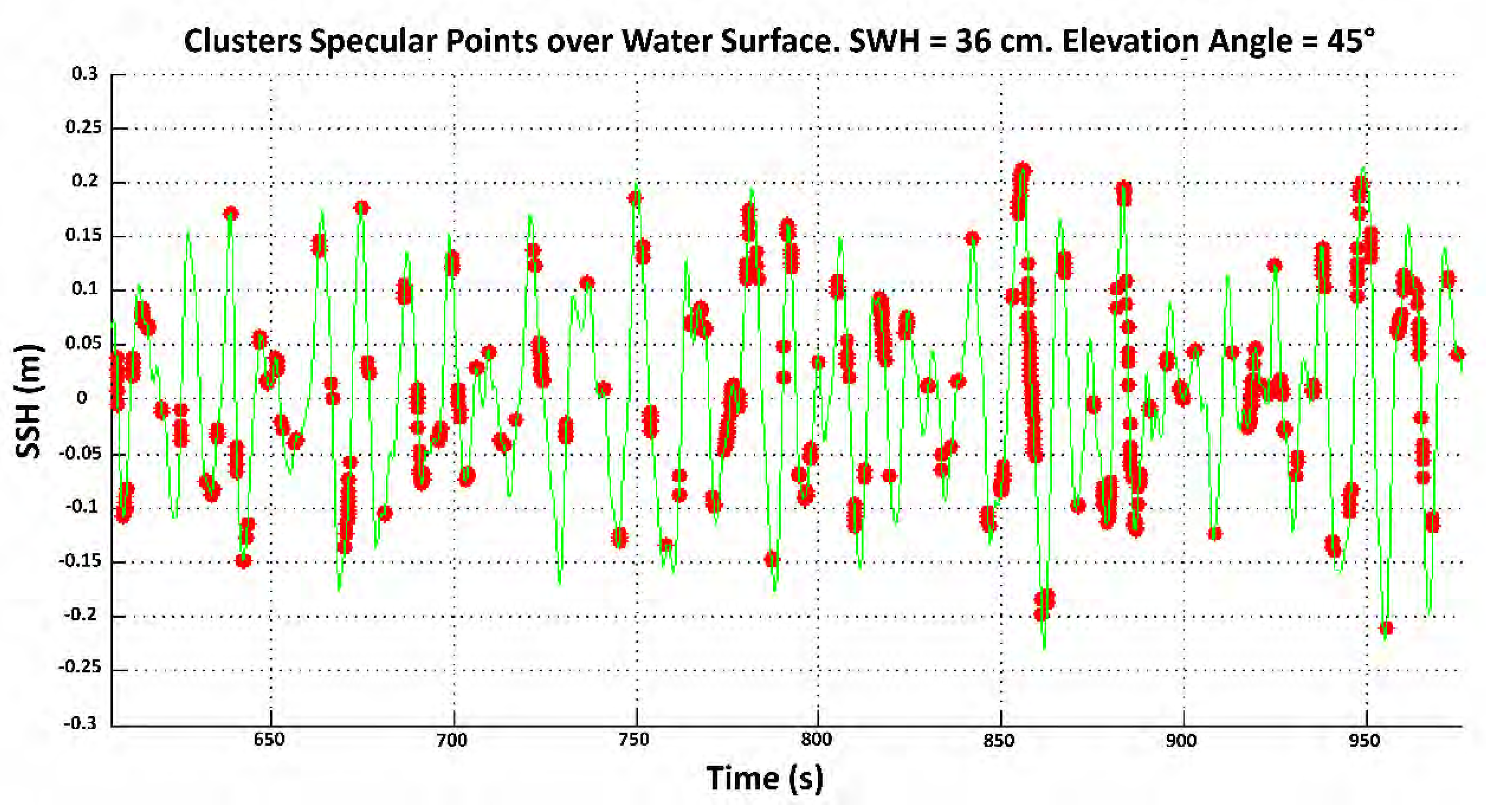
The specular points are identified continuously every 20 ms over the spatial (to transform the temporal domain into spatial surface profile, a celerity value of 1.6 m/s was used, since this was the only data available from the wave probe) surface profile when the local incident (${\text{θ}}_{\text{i}}$) and the scattered (${\text{θ}}_{\text{s}}$) angles are the same. The distribution of the specular points is not uniform, being characterized by different clusters (Figure 5). 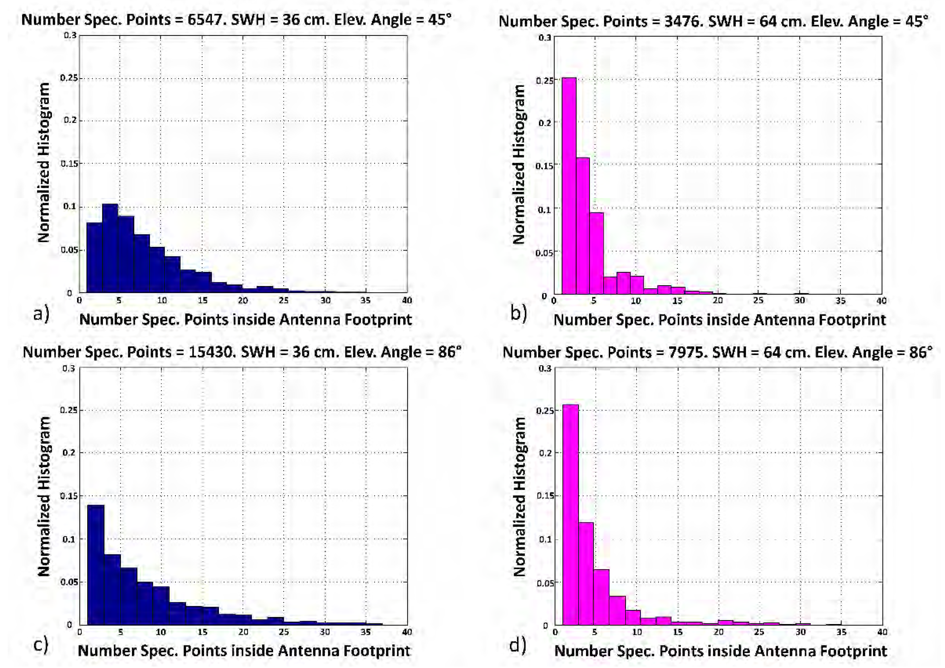This experimental result shows the micro-Doppler phenomenon [31] due to the small oscillations of the surface roughness. The normalized histograms of the number of specular points inside the antenna footprint every 20 ms are shown in Figure 6a–d for SWH = 36 cm and ${\text{θ}}_{\text{e}}$ = 45°, SWH = 64 cm and ${\text{θ}}_{\text{e}}$ = 45°, SWH = 36 cm and ${\text{θ}}_{\text{e}}$ = 86°, SWH = 64 cm and ${\text{θ}}_{\text{e}}$ = 86°, respectively. The number of clusters with a high number of specular points is larger for lower SWH. Additionally, it is derived that the total number of specular points is larger for lower SWH and for larger elevation angles. Local diffraction effects [26] contribute to the time-continuous uninterrupted ‘sea’ surface height (SSH) measurements provided by the PYCARO reflectometer (Figure 7).

Figure 5. Clusters of specular points distributed over the water surface profile as computed using the temporal series of data provided from the HR Wallingford wave probe monitor for a SWH = 36 cm and ${\text{θ}}_{\text{e}}$= 45°. SSH, sea surface height.

Figure 5. Clusters of specular points distributed over the water surface profile as computed using the temporal series of data provided from the HR Wallingford wave probe monitor for a SWH = 36 cm and ${\text{θ}}_{\text{e}}$= 45°. SSH, sea surface height.

Figure 6. Specular points distribution computed using the temporal series of data provided from the HR Wallingford wave probe monitor for a: (a) SWH = 36 cm and ${\text{θ}}_{\text{e}}$ = 45°; (b) SWH = 64 cm ${\text{θ}}_{\text{e}}$ = 45°; (c) SWH = 36 cm and ${\text{θ}}_{\text{e}}$ = 86°; and (d) SWH = 64 cm and ${\text{θ}}_{\text{e}}$= 86°.

Figure 6. Specular points distribution computed using the temporal series of data provided from the HR Wallingford wave probe monitor for a: (a) SWH = 36 cm and ${\text{θ}}_{\text{e}}$ = 45°; (b) SWH = 64 cm ${\text{θ}}_{\text{e}}$ = 45°; (c) SWH = 36 cm and ${\text{θ}}_{\text{e}}$ = 86°; and (d) SWH = 64 cm and ${\text{θ}}_{\text{e}}$= 86°.

Figure 7. Analysis of the electromagnetic interaction of the GPS signals and the scattering surface in a bistatic scenario. The phase (after retracking) distribution of the scattered field is time- and space-located over the temporal evolution of the SSH as measured by the PYCARO reflectometer. This analysis has been performed with a SWH = 36 cm and an elevation angle of ${\text{θ}}_{\text{e}}$ = 86°.

Figure 7. Analysis of the electromagnetic interaction of the GPS signals and the scattering surface in a bistatic scenario. The phase (after retracking) distribution of the scattered field is time- and space-located over the temporal evolution of the SSH as measured by the PYCARO reflectometer. This analysis has been performed with a SWH = 36 cm and an elevation angle of ${\text{θ}}_{\text{e}}$ = 86°.

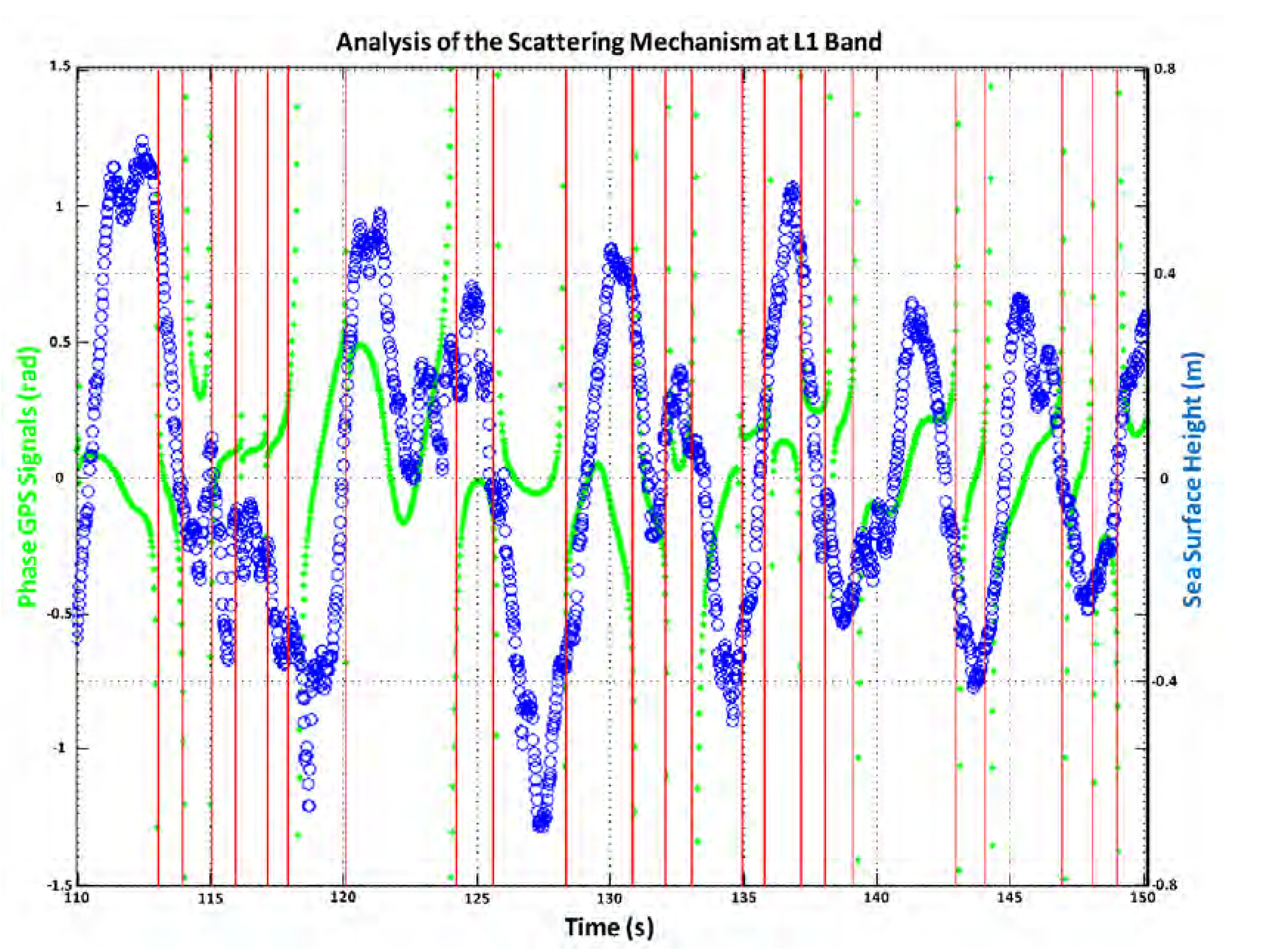
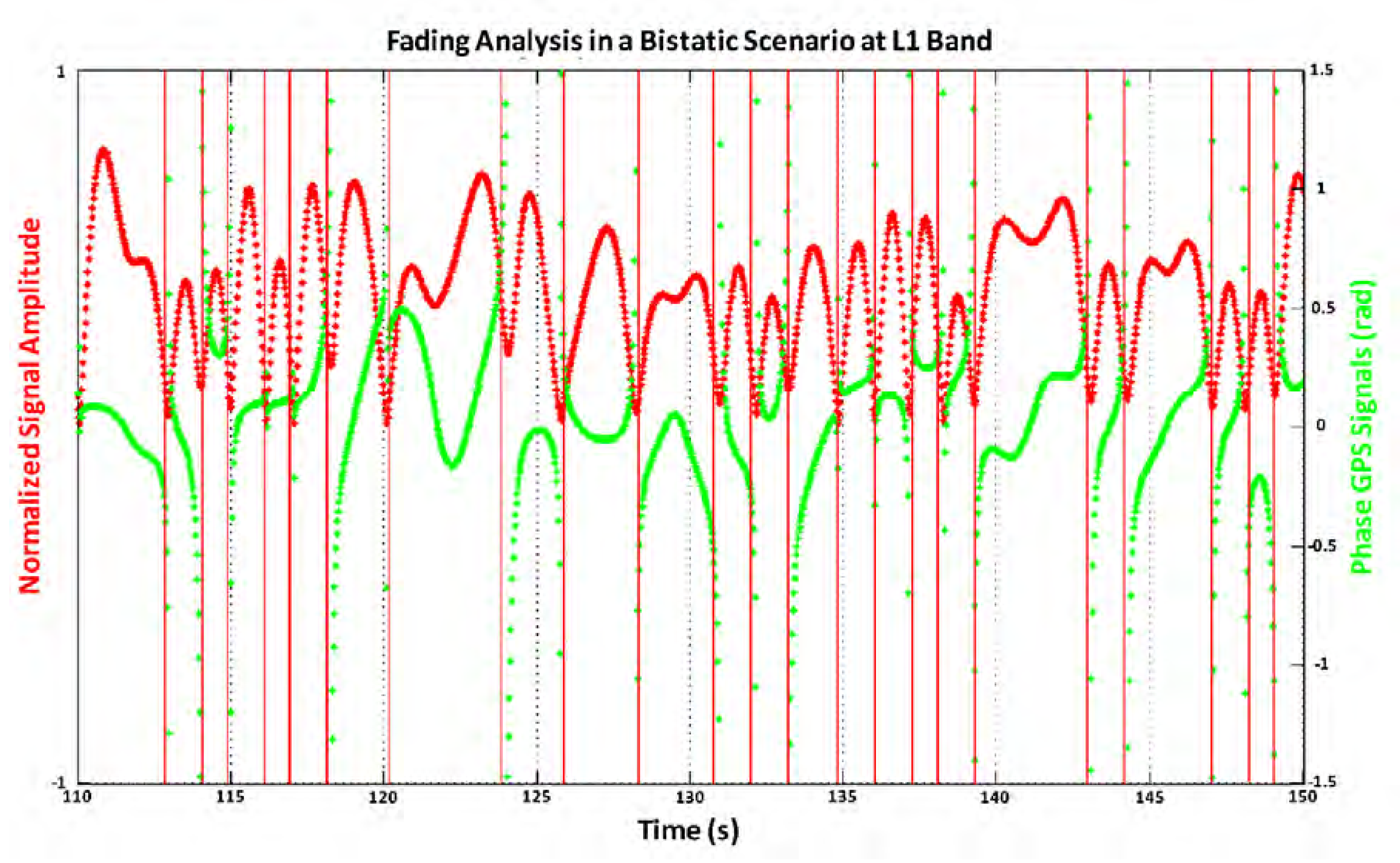
Figure 7 shows the SSH as measured by PYCARO for a SWH = 36 cm and ${\text{θ}}_{\text{e}}$= 86°. The total phase is important, but here, we are inferring surface deviations from phase changes only of the waveform peak. Any contribution (secondary specular points) away from the nominal one adds power at the trailing edge of the waveform, although very close to the main peak due to the short differential delay. This process distorts the waveform, and the peak becomes rounder. The one-sigma rms of the altimetric information is ~1 cm. Note that the sign of the phase of the received GPS signals (after retracking) changes at the wave valleys and crests, that is when the surface starts “approaching” the receiver or it starts “moving away” from it. These changes in the phase of the signals after being retracked are related to the relative velocity of the target with respect to the receiver (induced Doppler frequency shift). Some of these changes are associated with the larger waves, but others with smaller waves that also produce changes in the relative velocity of the specular points with respect to PYCARO. Each specular point has a different relative phase, which contributes to the speckle noise, responsible for the power fluctuations in the reflected signals (see the vertical red lines in Figure 8).

Figure 8. Normalized reflected signal power amplitude fluctuations due to the phase (after retracking) changes induced by the scattering surface. This analysis has been performed with a SWH = 36 cm and an elevation angle of ${\text{θ}}_{\text{e}}$ = 86°.

Figure 8. Normalized reflected signal power amplitude fluctuations due to the phase (after retracking) changes induced by the scattering surface. This analysis has been performed with a SWH = 36 cm and an elevation angle of ${\text{θ}}_{\text{e}}$ = 86°.

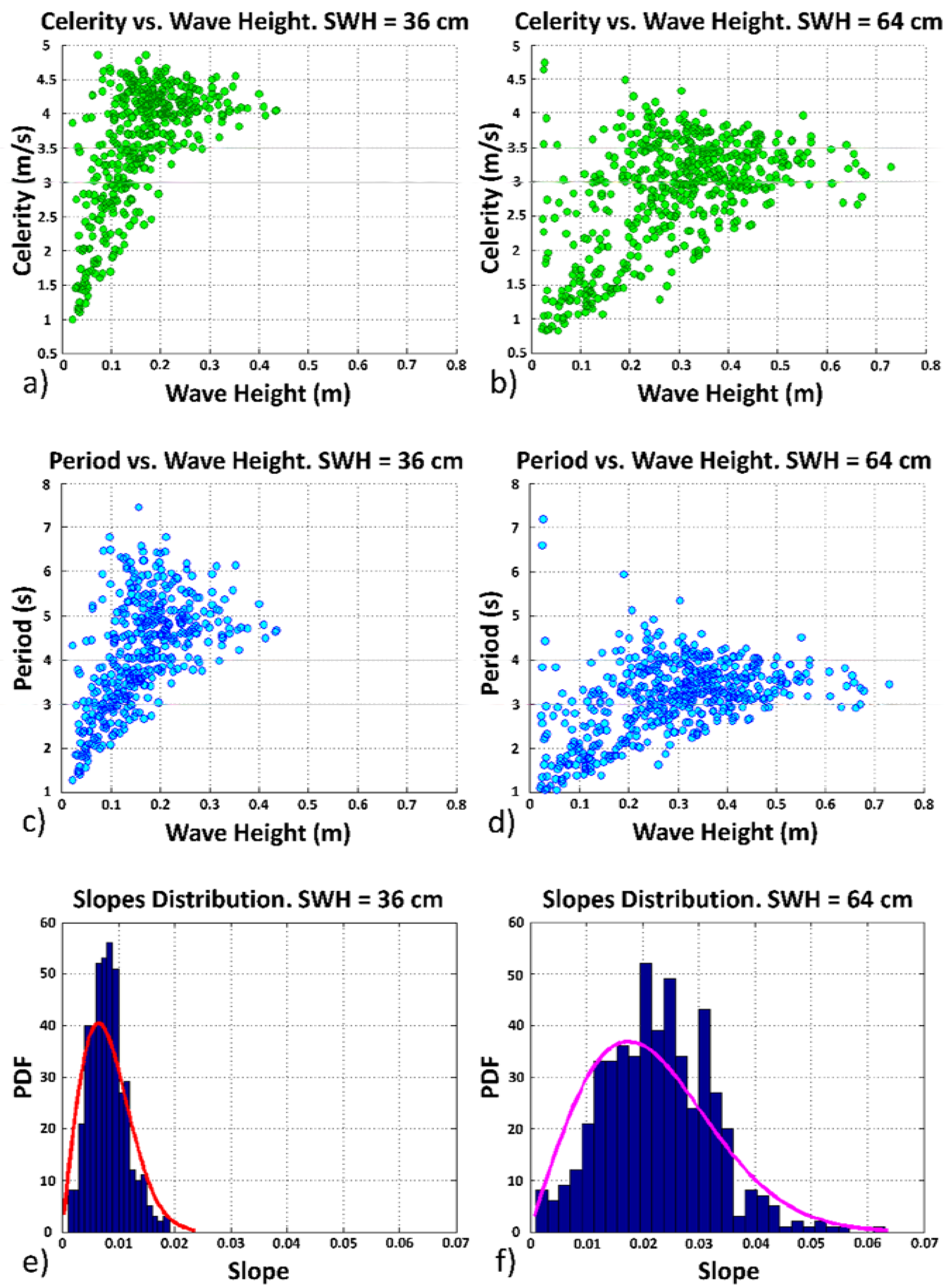
The number of scatterers ${\text{N}}_{\text{n}}$ is related to the sea surface motion through the appearance and disappearance of specular points [32]. In the CIEM experiment, this process was mostly due to the travel of the water waves. During a wave period, some specular points moved outside the antenna footprint, and others moved inside from a neighboring footprint. The maximum measured value of the slopes was 0.02 and 0.06, for a SWH = 36 cm and for a SWH = 64 cm, respectively (Figure 4e,f). The waves were identified using the so-called zero-down-crossing method [33], which includes the celerities in the computation of the slopes (the horizontal scale threshold of the slopes’ pdf was ~1.7 m). The region on the surface that contributed in-phase to the reflected signal was actually a smaller region (scattering cell) than the first Fresnel zone, larger for higher values of SWH (Table 1). Larger SWH values led to larger scattering cell over the water surface.

3.2. Water Surface Height Measurements

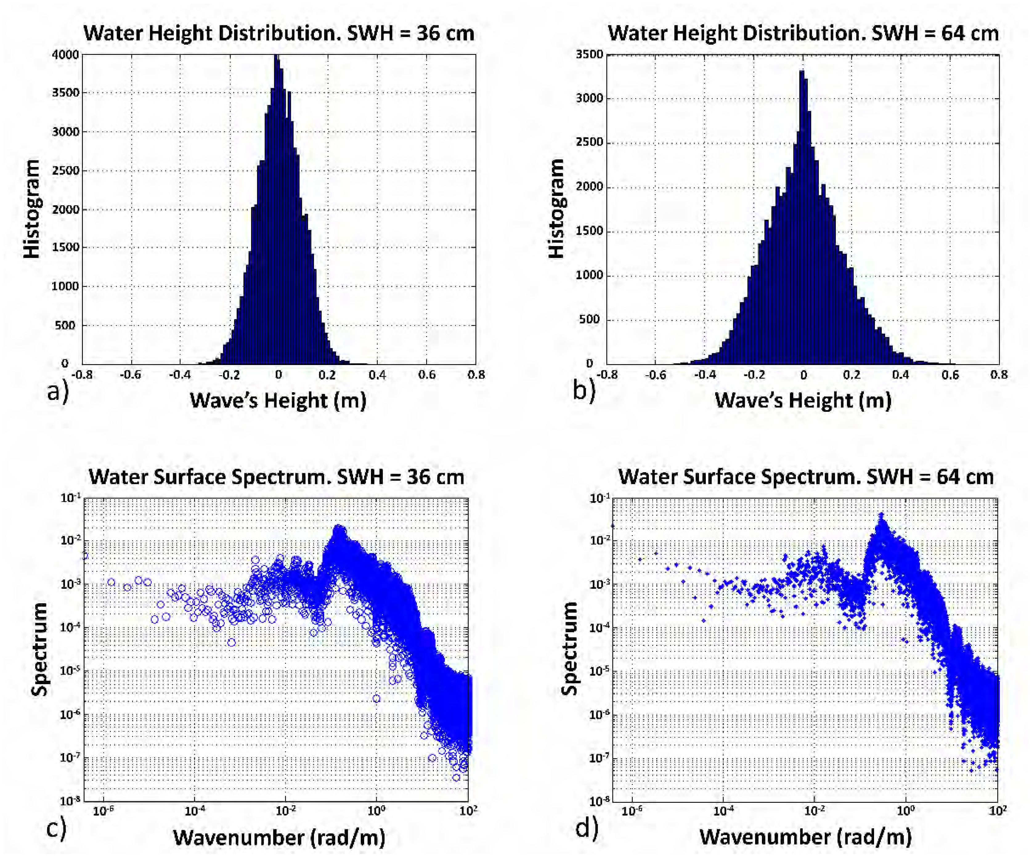
The performance of the PYCARO instrument has been evaluated for low-altitude applications (e.g., coastal applications). The experiment and the dataset generation were performed in a controlled manner. The height distributions of the two surface states obtained using the HR Wallingford wave probe are represented in Figure 9a,b. Their corresponding water surface spectra were derived from the time series provided by this sensor (Figure 9c,d).

Figure 9. Surface height distributions obtained using the HR Wallingford wave probe monitor for a: (a) SWH = 36 cm and (b) SWH = 64 cm. Corresponding wave surface spectra for a: (c) SWH = 36 cm and (d) SWH = 64 cm at the CIEM.

Figure 9. Surface height distributions obtained using the HR Wallingford wave probe monitor for a: (a) SWH = 36 cm and (b) SWH = 64 cm. Corresponding wave surface spectra for a: (c) SWH = 36 cm and (d) SWH = 64 cm at the CIEM.

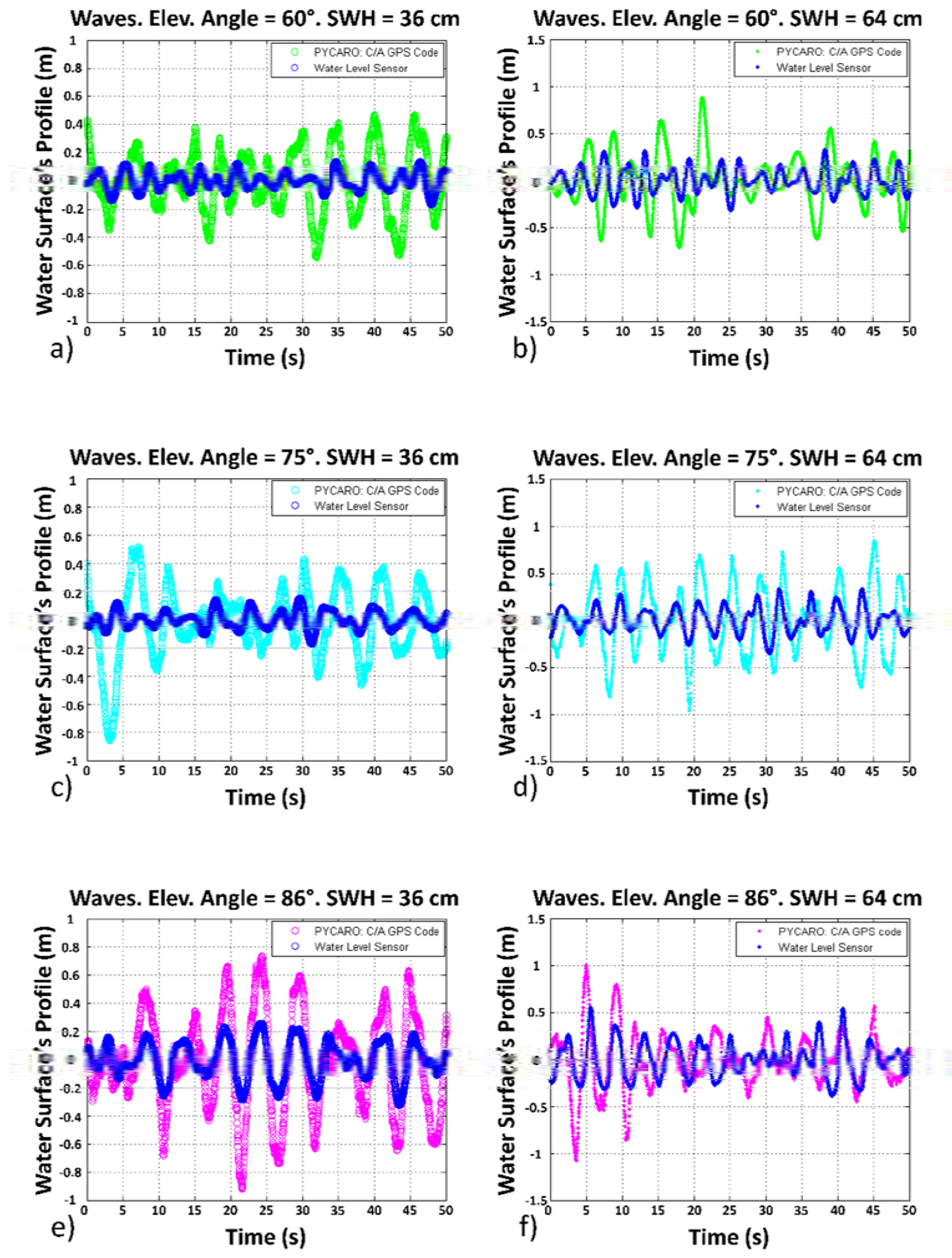
As a first step, the scattering in the time domain for different water surface states and transmitter elevation angles is analyzed. The instantaneous SSH relative to the mean water level in the channel as measured by the water level sensor and that derived using PYCARO (from the C/A code) are presented in Figure 10a,c,e for a SWH = 36 cm, and in Figure 10b,d,f for a SWH = 64 cm, respectively, for different elevation angles: ${\text{θ}}_{\text{e}}$= 60°, 75° and 86°.

The curve defined by the evolution in time of the geometric ranges (after scattering over the water surface) between the “GPS satellite” (transmitter) and the PYCARO instrument (receiver) was detrended to obtain the SSH. As can be seen, the wave profile as measured by the level sensor (Figure 10) is correlated with the one derived from PYCARO’s observables obtained from the C/A code. (However, the amplitude estimated from PYCARO [14] is larger than that from the gauges. A similar behavior was observed in a field experiment over the Mediterranean Sea using the GPS C/A code, but not with the GPS P(Y) code [14].)

Figure 10. For an elevation angle of (a,b) ${\text{θ}}_{\text{e}}$= 60°, (c,d) ${\text{θ}}_{\text{e}}$= 75° and (e,f) ${\text{θ}}_{\text{e}}$= 86°, (a,c,e) sample wave profile as measured by PYCARO using the GPS C/A code and by the water level sensor for a SWH = 36 cm and (b,d,f) for SWH = 64 cm.

Figure 10. For an elevation angle of (a,b) ${\text{θ}}_{\text{e}}$= 60°, (c,d) ${\text{θ}}_{\text{e}}$= 75° and (e,f) ${\text{θ}}_{\text{e}}$= 86°, (a,c,e) sample wave profile as measured by PYCARO using the GPS C/A code and by the water level sensor for a SWH = 36 cm and (b,d,f) for SWH = 64 cm.

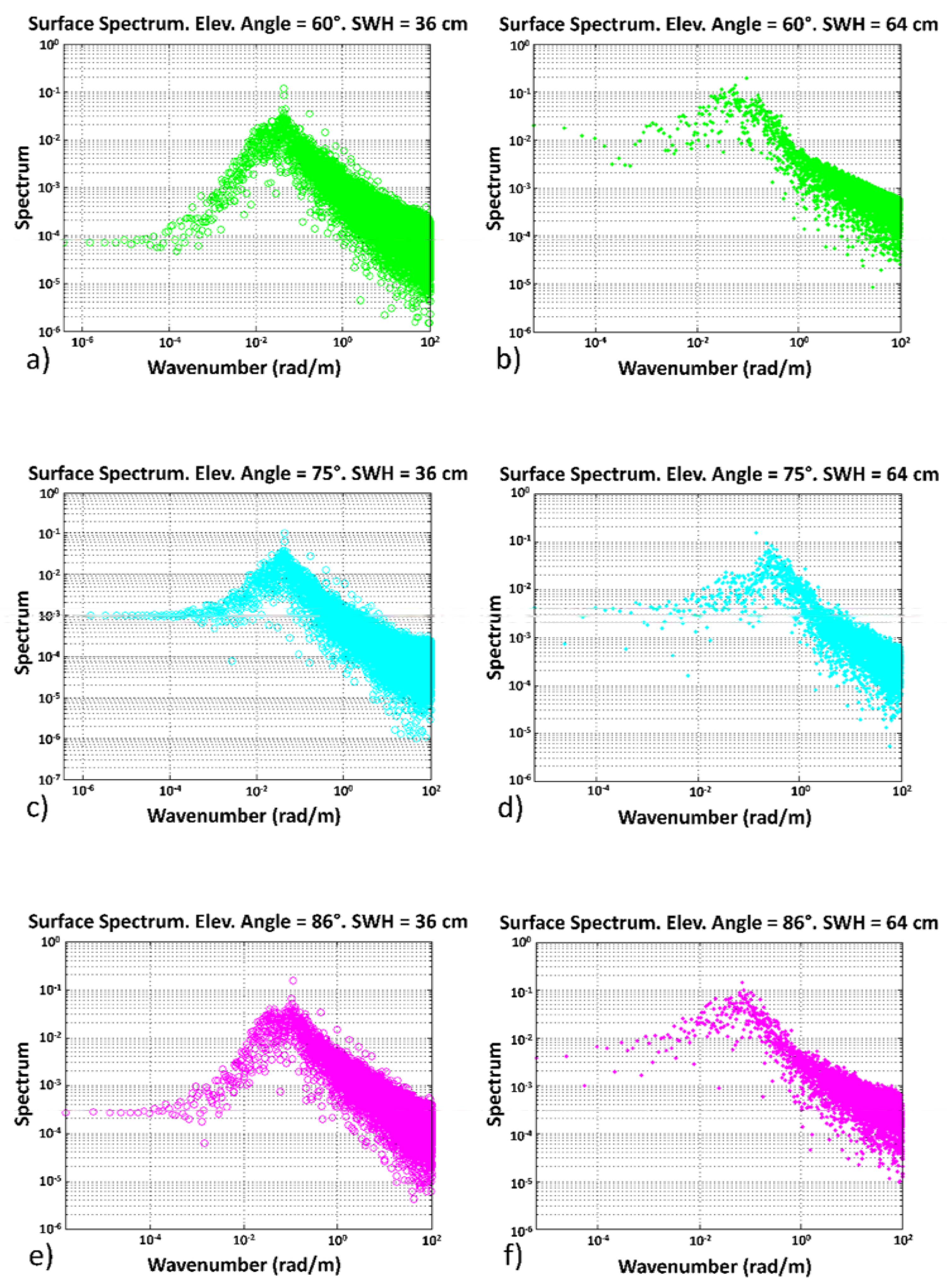
Additionally, the water surface’s spectra computed for the different surface states as measured by PYCARO for the different elevation angles (${\text{θ}}_{\text{e}}$= 60°, 75° and 86°) are represented in Figure 11a,c,e and Figure 11b,d,f respectively, for a SWH = 36 cm and 64 cm. The Pearson’s linear correlation coefficients of the level gauge sensor and the bistatically-derived results are 0.78, 0.85 and 0.81 for a SWH = 36 cm and 0.34, 0.74 and 0.72 for a SWH = 64 cm, ${\text{θ}}_{\text{e}}$= 60°, 75° and 86°.

Figure 11. For an elevation angle of (a,b) ${\text{θ}}_{\text{e}}$= 60°, (c,d) ${\text{θ}}_{\text{e}}$= 75° and (e,f) ${\text{θ}}_{\text{e}}$= 86°, (a,c,e) water surface spectra as measured by PYCARO using the GPS C/A code for SWH = 36 cm and (b,d,f) for SWH = 64 cm.

Figure 11. For an elevation angle of (a,b) ${\text{θ}}_{\text{e}}$= 60°, (c,d) ${\text{θ}}_{\text{e}}$= 75° and (e,f) ${\text{θ}}_{\text{e}}$= 86°, (a,c,e) water surface spectra as measured by PYCARO using the GPS C/A code for SWH = 36 cm and (b,d,f) for SWH = 64 cm.

3.3. Analysis of the Coherent and Incoherent Components after Retracking

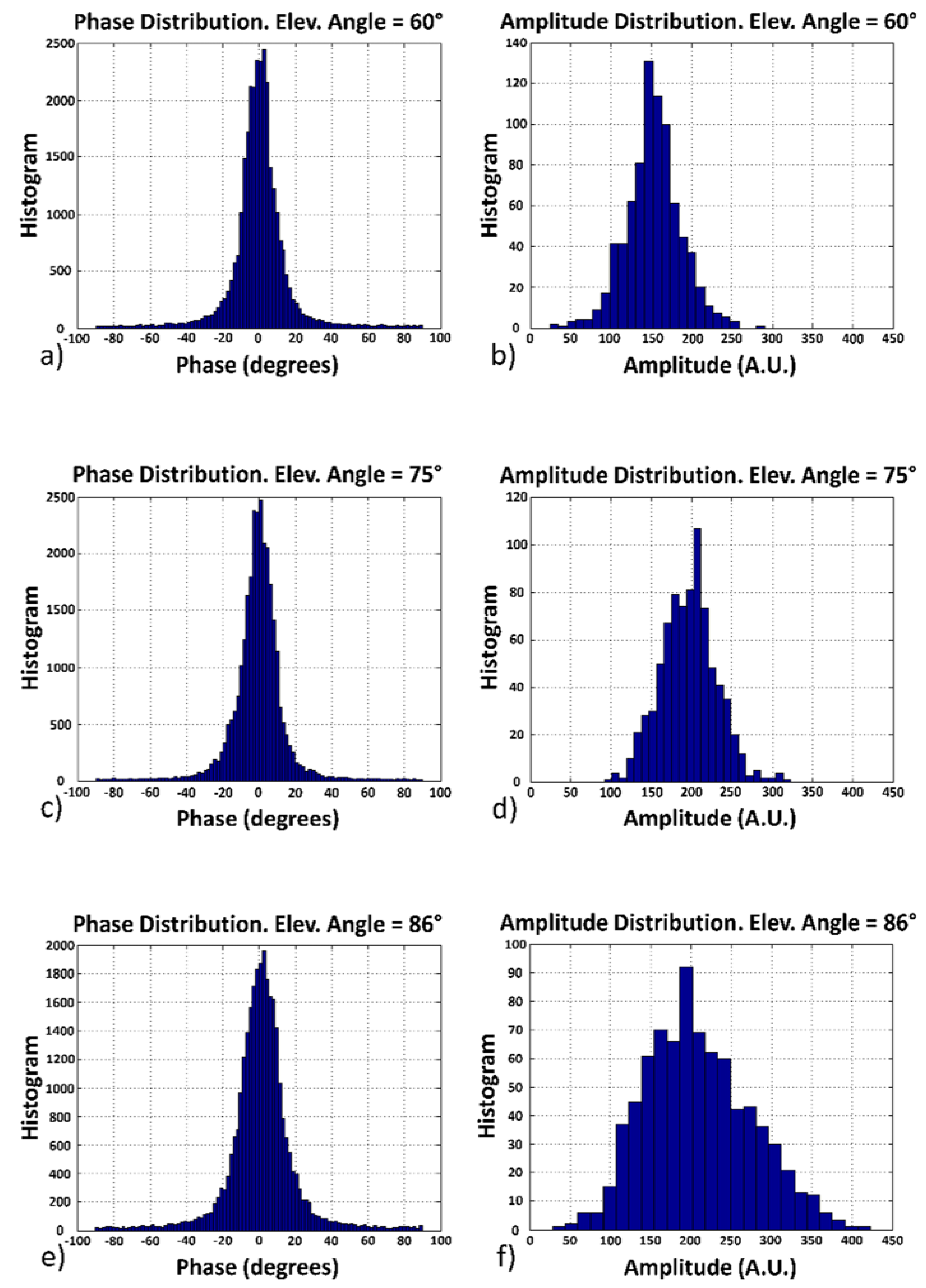
The phase of the signals after complex cross-correlation with the locally-generated C/A code and after retracking (Figure 12a,c,e) for different elevation angles (${\text{θ}}_{\text{e}}$= 60°, 75° and 86°) and for a SWH = 36 cm is studied in this section. The retracking algorithm implemented in the PYCARO reflectometer tends to align the sum of the I and Q components of the scattered field with the I axis and switches 180° during each data bit reversal. The GPS satellites’ motion (and eventually, the receiver’s motion, as well) induces a change in the delay and the phase difference of the waveforms that needs to be compensated for the coherent and incoherent averaging.

Figure 12. At an elevation angle of (a,b) ${\text{θ}}_{\text{e}}$= 60°, (c,d) ${\text{θ}}_{\text{e}}$= 75° and (e,f) ${\text{θ}}_{\text{e}}$= 86°, (a,c,e) histogram of the phase and (b,d,f) amplitude of the signals after retracking for a SWH = 36 cm.

Figure 12. At an elevation angle of (a,b) ${\text{θ}}_{\text{e}}$= 60°, (c,d) ${\text{θ}}_{\text{e}}$= 75° and (e,f) ${\text{θ}}_{\text{e}}$= 86°, (a,c,e) histogram of the phase and (b,d,f) amplitude of the signals after retracking for a SWH = 36 cm.

The length of the dataset is 30 min, sampled at 10 Hz, showing that the random complex vectors add up together, privileging a certain direction in the complex plane (Figure 12a,c,e). As can be appreciated, the phase’s standard deviation of the retracked signals is actually quite small, which shows a strong coherent component being tracked. As the elevation angle increases from ${\text{θ}}_{\text{e}}$ = 60° − 86°, the phase standard deviation increases also from 13.4° to 19.1° (Figure 12a,c,e and Table 2), and the kurtosis decreases from 17.5 to 8.5 (Table 2). This is a clear indication that the amount of incoherent scattering increases (the pdf becomes more like a Gaussian one), due to the larger contribution of the wave crests and valleys at larger elevation angles. This is also in agreement with the evolution of the amplitude distribution, which tends to a Rayleigh distribution, as the elevation angle increases (Figure 12b,d,f and Table 3).

Table 2. Statistical analysis of the phase (after retracking) distribution of the scattered GPS signals over the CIEM wave channel at different elevation angles: ${\text{θ}}_{\text{e}}$= 60°, 75° and 86°.

${\text{θ}}_e$ (Degrees)	60°	75°	86°
Phase SD (Degrees)	13.4°	17.4°	19.1°
Phase Mean (Degrees)	0.9°	−0.5°	1.2°
Phase Kurtosis	17.5	10.4	8.5
Phase Skewness	0.9	−0.06	−0.05

Table 2. Statistical analysis of the phase (after retracking) distribution of the scattered GPS signals over the CIEM wave channel at different elevation angles: ${\text{θ}}_{\text{e}}$= 60°, 75° and 86°.

${\text{θ}}_e$ (Degrees)	60°	75°	86°
Phase SD (Degrees)	13.4°	17.4°	19.1°
Phase Mean (Degrees)	0.9°	−0.5°	1.2°
Phase Kurtosis	17.5	10.4	8.5
Phase Skewness	0.9	−0.06	−0.05

Table 3. Statistical analysis of the amplitude (after retracking) distribution of the scattered GPS signals over the CIEM wave channel at different elevation angles: ${\text{θ}}_{\text{e}}$= 60°, 75° and 86°.

${\text{θ}}_e$ (Degrees)	60°	75°	86°
Amplitude SD (A.U.)	34	37	65
Amplitude Mean (A.U.)	152	195	209
Amplitude Kurtosis	3.91	3.44	2.74
Amplitude Skewness	−0.013	0.05	0.324

Table 3. Statistical analysis of the amplitude (after retracking) distribution of the scattered GPS signals over the CIEM wave channel at different elevation angles: ${\text{θ}}_{\text{e}}$= 60°, 75° and 86°.

${\text{θ}}_e$ (Degrees)	60°	75°	86°
Amplitude SD (A.U.)	34	37	65
Amplitude Mean (A.U.)	152	195	209
Amplitude Kurtosis	3.91	3.44	2.74
Amplitude Skewness	−0.013	0.05	0.324

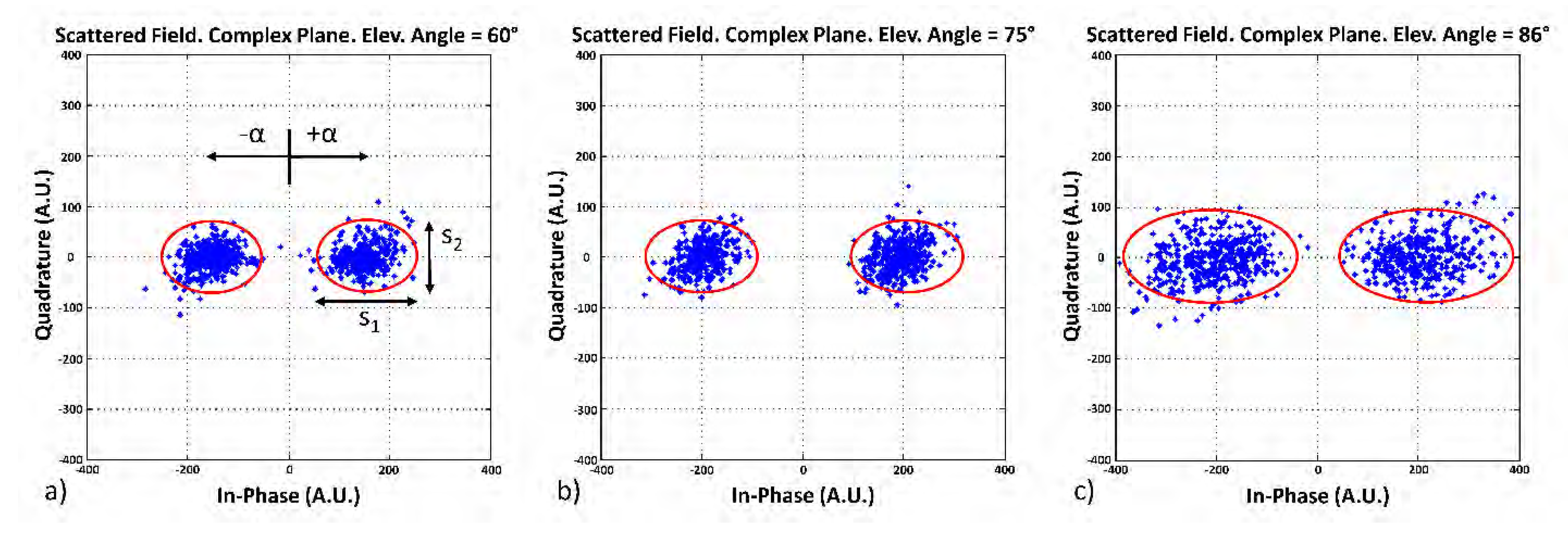
The ratio of the coherent-to-incoherent components as seen by the PYCARO instrument is derived using the total scattered field complex plane representation (Figure 13). Each single measurement of the scattered complex field during the 30 min is represented. For a completely incoherent scattering, the distribution in the complex plane of the scattered field should theoretically follow a zero-mean two-dimensional Gaussian distribution with variances ${\text{s}}_1$ and ${\text{s}}_2$ [30] (p. 125). However, experimental results (Figure 13a–c) show that after retracking, the total scattered field is displaced from the center by a certain value ±$\text{α}$ in the real axis (equal to the mean of the amplitude distribution) into two regions with an ellipsoidal shape, which proves the presence of a strong coherent component in the specular direction. As explained before, the phase changes (Figure 13a–c) are due to changes of the navigation bit sign and the effect of the speckle noise. Thus, there are two regions displaced ±$\text{α}$ from the center. The relative weight of the coherent-to-incoherent components is quantified by the $\text{B}$ parameter [30] (p. 126):

$${\text{B}}^2=\frac{{\text{α}}^2}{{\text{s}}_1+{\text{s}}_2}$$

(3)

Note that $\text{B}$ tends to ∞ for a totally coherent field (${\text{s}}_1={\text{s}}_2=$ 0) and it is equal to zero for a totally incoherent field ($\text{α}$ = 0). The results from this experiment show that the weight of the coherent component ($\text{B}$) reduces by ~6% (from 0.97 to 0.95) when the elevation angle increases from ${\text{θ}}_{\text{e}}$= 60° − 86° (Table 4), while the incoherent scattering increases as the surface roughness increases, in agreement with the reduction of the asymmetry factor $\text{K}\cong \raisebox{1ex}{${\text{s}}_1$}\!\left/ \!\raisebox{-1ex}{${\text{s}}_2$}\right.$ (Table 4). At the same time, the larger the elevation angle, the larger the phase noise because of a larger ‘apparent’ water surface roughness, but still much lower than the amplitude standard deviation.

Figure 13. Scattered field complex plane representation for a SWH = 36 cm at an elevation angle of ${\text{θ}}_{\text{e}}$= 60° (a), 75° (b) and 86° (c).

Figure 13. Scattered field complex plane representation for a SWH = 36 cm at an elevation angle of ${\text{θ}}_{\text{e}}$= 60° (a), 75° (b) and 86° (c).

Table 4. Statistical analysis of the complex field distribution of the scattered GPS signals after retracking, over the CIEM wave channel at different elevation angles: ${\text{θ}}_{\text{e}}$= 60°, 75° and 86°.

${\text{θ}}_e$ (Degrees)	60°	75°	86°
Coherent Scattering: ${\text{α}}^2$ (A.U.)	22,939	37,725	43,992
Incoherent Scattering: ${\text{ s}}_1+{\text{s}}_2$ (A.U.)	23,648	38,392	46,307
Ratio Coherent to Incoherent Scattering: ${\text{B}}^2={\text{α}}^2/{\text{s}}_1+{\text{s}}_2$ (A.U.)	0.97	0.97	0.95
Asymmetry Factor: $\text{K}\cong {\text{s}}_1/{\text{s}}_2$	39	39	30

Table 4. Statistical analysis of the complex field distribution of the scattered GPS signals after retracking, over the CIEM wave channel at different elevation angles: ${\text{θ}}_{\text{e}}$= 60°, 75° and 86°.

${\text{θ}}_e$ (Degrees)	60°	75°	86°
Coherent Scattering: ${\text{α}}^2$ (A.U.)	22,939	37,725	43,992
Incoherent Scattering: ${\text{ s}}_1+{\text{s}}_2$ (A.U.)	23,648	38,392	46,307
Ratio Coherent to Incoherent Scattering: ${\text{B}}^2={\text{α}}^2/{\text{s}}_1+{\text{s}}_2$ (A.U.)	0.97	0.97	0.95
Asymmetry Factor: $\text{K}\cong {\text{s}}_1/{\text{s}}_2$	39	39	30

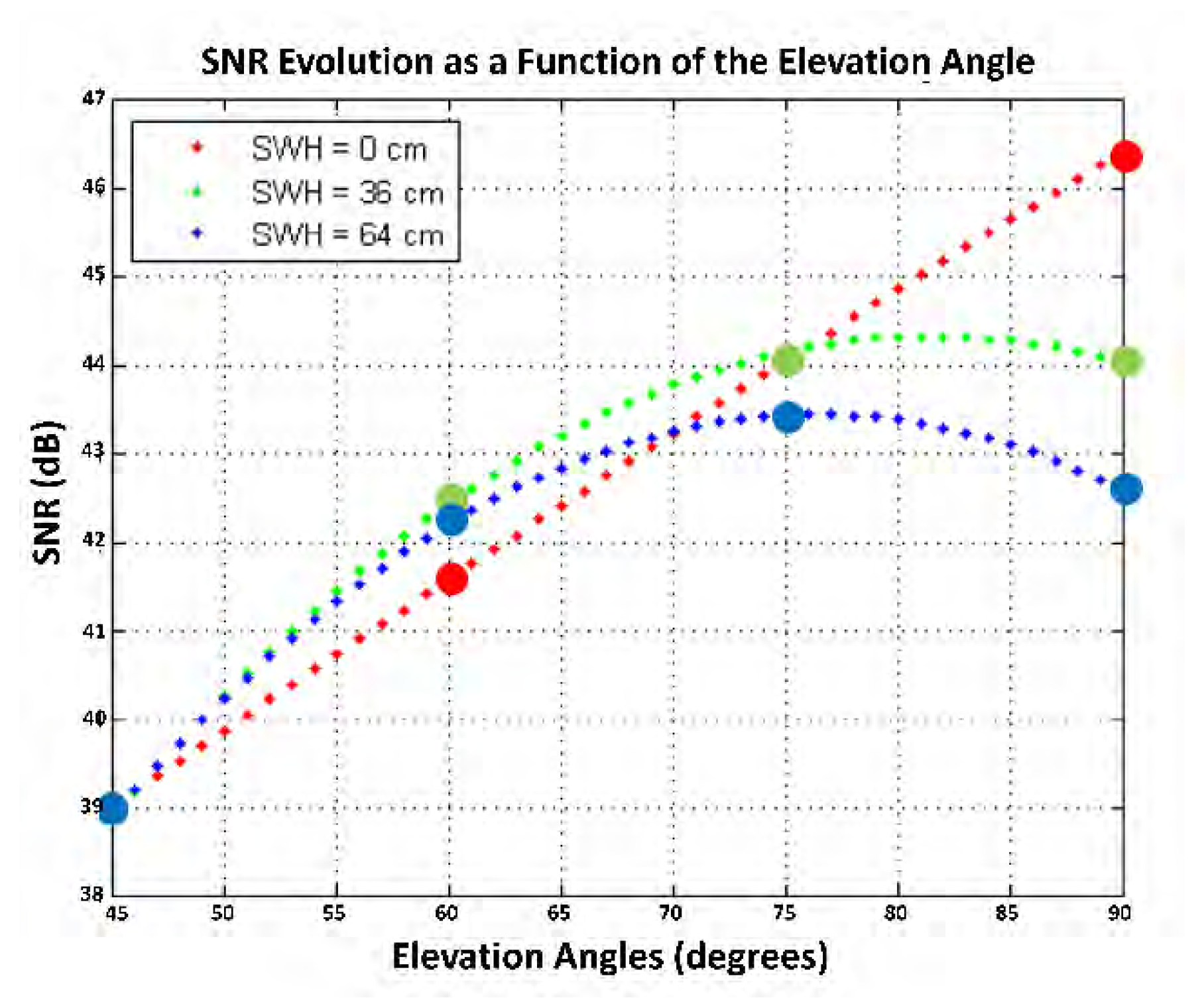
Figure 14. SNR of the reflected signal for three different surface states and for an elevation angle in the range from ${\text{θ}}_{\text{e}}$= 45° to ${\text{θ}}_{\text{e}}$ = 86°. The figure was obtained using a best-fit approximation of the experimental data over elevation angles at ${\text{θ}}_{\text{e}}$= 45°, ${\text{θ}}_{\text{e}}$= 60°, ${\text{θ}}_{\text{e}}$= 75° and ${\text{θ}}_{\text{e}}$= 86°.

Figure 14. SNR of the reflected signal for three different surface states and for an elevation angle in the range from ${\text{θ}}_{\text{e}}$= 45° to ${\text{θ}}_{\text{e}}$ = 86°. The figure was obtained using a best-fit approximation of the experimental data over elevation angles at ${\text{θ}}_{\text{e}}$= 45°, ${\text{θ}}_{\text{e}}$= 60°, ${\text{θ}}_{\text{e}}$= 75° and ${\text{θ}}_{\text{e}}$= 86°.

The signal-to-noise ratio (SNR) of the scattered field increases with increasing elevation angles (Figure 14). The SNR evolution as a function of the elevation angle is derived using a best-fit approximation of the experimental data at ${\text{θ}}_{\text{e}}$ = 45°, 60°, 75° and 86°. For elevation angles ${\text{θ}}_{\text{e}}$larger than 60° the value of the SNR decreases with increasing values of the SWH (Figure 14), because of the larger phase standard deviation (Figure 13a–c). However, for lower elevation angles, the SNR tends to the same value in both cases: rough and flat surfaces.

3.4. Evaluation of the Effective Small-Scale Surface Roughness

In order to compare GPS scattering data with a simple theoretical model, effective sea surface parameters are introduced [34]. However, these parameters cannot be applied away from the specular direction, because they depend on the geometry [35]. The reflectivity of the coherent scattering component can be derived as [36] (p. 1008):

$${\text{Γ}}_{\text{rl}}^{\text{coh}}={\left|{\mathfrak{N}}_{\text{rl}}\left({\text{θ}}_{\text{e}}\right)\right|}^2{\text{e}}^{-{\left(2{\text{σksinθ}}_{\text{e}}\right)}^2}$$

(4)

where subscripts $\text{r}$ and $\text{l}$ denote the incident polarization (right-hand circular polarization) and the scattered polarization (left-hand circular polarization), respectively, ${\mathfrak{N}}_{\text{rl}}$ is the Fresnel reflection coefficient, $\text{σ}$ is the surface height standard deviation and $\text{k}$ is the wavenumber. Note that for a flat surface, the surface height standard deviation (surface roughness) $\text{σ}$ is zero, and the reflectivity reduces to the square of the amplitude of the Fresnel reflection coefficient. The phase standard deviation of the peak of the complex cross-correlation with the locally-generated C/A code before it is aligned (obviously with some residual noise) to the I axis was computed during the experiment (Figure 4.14 in Enric Valencia’s PhD Thesis [37] or Figure 3a in [38] illustrates this point; there, due to the movement of the transmitter, the phase also varied with time), in addition to the measurements of the phase after retracking. The experimental distributions of the before-retracking phase standard deviation ${\text{σ}}_{\text{ϕ}}$ are linked to the rms surface height (The low elevation of the antenna acts as a high-pass filter. SWH is mainly determined by the large-scale waves; waves with larger periods, larger heights and also with higher celerities (Figure 4). The small-scale rms surface heights values corresponding to the peak of the distributions (~3.1 cm, ~3.1 cm, ~4.4 cm and ~7.2 cm) are the same for both SWH = 36 cm and SWH = 64 cm) (dispersion of the height’s distribution of the small-scale waves) as [30] (p. 246):

$$\text{σ}=\frac{{\text{σ}}_{\text{ϕ}}}{2{\text{ksinθ}}_{\text{e}}}$$

(5)

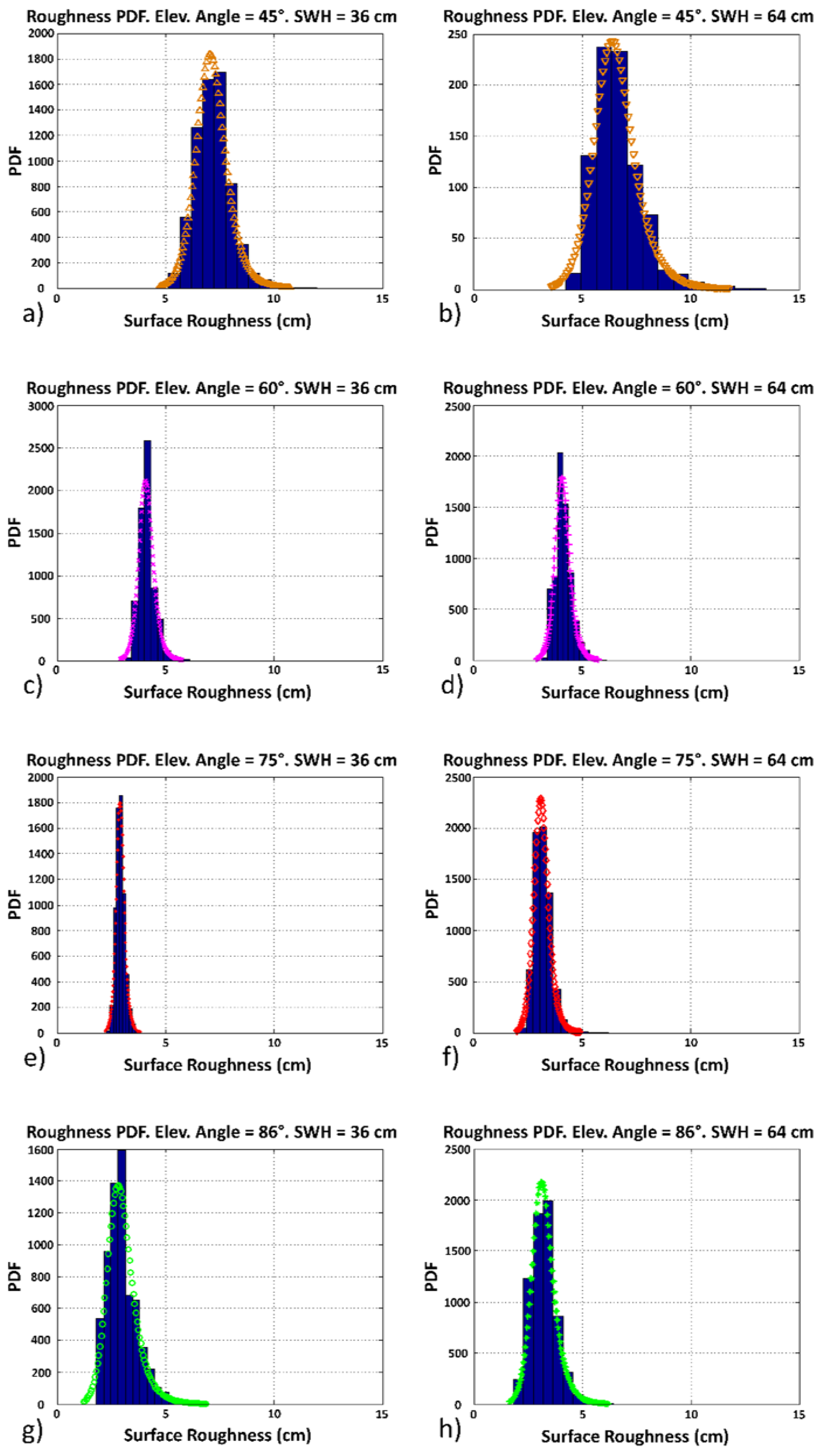
The small-scale surface roughness distributions (Equation (5)) are represented in Figure 15 for different elevation angles of ${\text{θ}}_{\text{e}}$ = 45°, 60°, 75° and 86°, for a SWH = 36 cm and 64 cm. These distributions are theoretically fitted by log-logistic pdfs (Figure 15) [39]. The small-scale surface roughness (rms surface height) values corresponding to the peak of the distributions are ~7.2 cm, ~4.4 cm, ~3.1 cm and ~3.1 cm for a SWH = 36 cm (Figure 15a,c,e,g respectively) and also for a SWH = 64 cm (Figure 15b,d,f,h respectively), for elevation angles of ${\text{θ}}_{\text{e}}$ = 45°, 60°, 75° and 86°, respectively. On the other hand, the theoretical roughness values corresponding to half of the coherent reflectivity decaying factor (Equation (4)) are ~1.75 cm, ~1.5 cm, ~1.25 cm and ~1.25 for elevation angles of ${\text{θ}}_{\text{e}}$ = 45°, 60°, 75° and 86°, respectively. Therefore, an experimental correction term $\text{P}$ could be derived from the ratio of the empirically-derived (Figure 15) to the theoretical small-scale surface roughness values (Table 5). This term is introduced to estimate the effective small scale roughness ${\text{σ}}_{\text{eff}}=\raisebox{1ex}{$\text{σ}$}\!\left/ \!\raisebox{-1ex}{$\text{P}$}\right.$. The difference between the effective small-scale roughness and the theoretical values is higher for lower elevation angles, as a factor of ~4.1 and ~2.5 for elevation angles of ${\text{θ}}_{\text{e}}$ = 45° and ${\text{θ}}_{\text{e}}$ = 86°, respectively.

Figure 15. Theoretical log-logistic pdf approximation to the small-scale surface roughness distributionsfor an elevation angle of (a,b) ${\text{θ}}_{\text{e}}$= 45° (c,d) ${\text{θ}}_{\text{e}}$= 60°, (e,f) ${\text{θ}}_{\text{e}}$= 75° and (g,h) ${\text{θ}}_{\text{e}}$= 86°; for (a,c,e,g) SWH = 36 cm and (b,d,f,h) for SWH = 64 cm. Note: the distributions of the small-scale surface roughness have been derived using the standard deviation of the signal before retracking.

Figure 15. Theoretical log-logistic pdf approximation to the small-scale surface roughness distributionsfor an elevation angle of (a,b) ${\text{θ}}_{\text{e}}$= 45° (c,d) ${\text{θ}}_{\text{e}}$= 60°, (e,f) ${\text{θ}}_{\text{e}}$= 75° and (g,h) ${\text{θ}}_{\text{e}}$= 86°; for (a,c,e,g) SWH = 36 cm and (b,d,f,h) for SWH = 64 cm. Note: the distributions of the small-scale surface roughness have been derived using the standard deviation of the signal before retracking.

Table 5. Theoretical and experimental small-scale roughness values and correction term for SWH = 36 cm and 64 cm for ${\text{θ}}_{\text{e}}$= 45°, 60°, 75° and 86°.

${\text{θ}}_e$ (Degrees)	45°	60°	75°	86°
Theoretical Small-Scale Roughness	1.75	1.5	1.25	1.25
Experimental Small-Scale Roughness (SWH = 36 cm)	7.2	4.4	3.1	3.1
Experimental Small Scale Roughness (SWH = 64 cm)	7.2	4.4	3.1	3.1
Correction Term $\text{P}$ (SWH = 36 cm)	4.1	2.9	2.5	2.5
Correction Term $\text{P}$ (SWH = 64 cm)	4.1	2.9	2.5	2.5

Table 5. Theoretical and experimental small-scale roughness values and correction term for SWH = 36 cm and 64 cm for ${\text{θ}}_{\text{e}}$= 45°, 60°, 75° and 86°.

${\text{θ}}_e$ (Degrees)	45°	60°	75°	86°
Theoretical Small-Scale Roughness	1.75	1.5	1.25	1.25
Experimental Small-Scale Roughness (SWH = 36 cm)	7.2	4.4	3.1	3.1
Experimental Small Scale Roughness (SWH = 64 cm)	7.2	4.4	3.1	3.1
Correction Term $\text{P}$ (SWH = 36 cm)	4.1	2.9	2.5	2.5
Correction Term $\text{P}$ (SWH = 64 cm)	4.1	2.9	2.5	2.5

3.5. Final Discussions

The first results show the feasibility of the PYCARO instrument operated in closed-loop mode for “sea” wave monitoring for long-term local sea level and wave monitoring. The correlation of the GNSS-R derived “sea” waves and the ground truth data show a dependence on the elevation angle and the SWH. The experiment in the CIEM wave channel provided a unique opportunity to demonstrate wave monitoring using closed-loop GNSS-R techniques as opposed to open-loop ones, which require an a priori approximate knowledge of the reflecting surface to perform the waveform tracking. In this work, the coherent scattering over the small-scale 1D mechanically-driven waves has been evaluated. A lower value of the effective small-scale roughness has been found as compared to the real water surface. The feasibility of local sea level monitoring using coherently reflected GPS C/A signals under large roughness conditions will also require a dedicated field experiment and further theoretical studies, but the application of GNSS-R to perform local sea level determination with the required precision for altimetric calibrations [17] is already promising.

4. Summary and Conclusions

A low-altitude GNSS-R like experiment has been performed in a controlled scenario in the CIEM wave channel at the premises of the Civil Engineering School of the UPC-BarcelonaTech using synthetic GPS data to mimic a realistic scenario. Two different water surface states with a SWH = 36 cm and 64 cm have been simulated for GPS “satellites” at elevation angles of ${\text{θ}}_{\text{e}}$ = 45°, 60°, 75° and 86°. The size of the scattering cells during the coherent integration time (${\text{T}}_{\text{c}}$= 20 ms) increases for larger scale surface roughness (SWH) and for decreasing elevation angles. The cell main axis is 0.22 m for a SWH = 36 cm and ${\text{θ}}_{\text{e}}$ = 86° and 1.36 m for a SWH = 64 cm and ${\text{θ}}_{\text{e}}$ = 45°. The Pearson’s linear correlation coefficients of the bistatically-derived SSH with the wave gauge data are 0.78, 0.85 and 0.81 for a SWH = 36 cm and 0.34, 0.74 and 0.72 for a SWH = 64 cm, respectively, for transmitter elevation angles of ${\text{θ}}_{\text{e}}$ = 60°, 75° and 86°, respectively. The ratio of the coherent-to-incoherent components of the scattered field after retracking was evaluated using a re-constructed field approach. In order to improve the statistical significance of the results, a 30 min long observation was acquired for each configuration. The ratio of the coherent-to-incoherent components as seen by the PYCARO reflectometer for a SWH = 36 cm is approximately ~ 1 in the range from ${\text{θ}}_{\text{e}}$ = 60° to ${\text{θ}}_{\text{e}}$ = 86°. As an independent scientific observable, the phase standard deviation of the GPS signals before retracking was computed during the experiment. Using these measurements, an estimation of the “facets” roughness (small-scale waves) was derived. Then, an empirical correction term to estimate the effective small-scale roughness was inferred comparing the experimental small-scale surface roughness data with those provided by the coherent reflectivity model derived under the KM scalar approximation. It depends on the satellite elevation angle and is as large as $\text{P}$ ~ 4.1 for ${\text{θ}}_{\text{e}}$= 45°. The lower value of the effective small-scale roughness at L1 as compared to the real water surface means that the scattering surface as seen by the GNSS-R instrument is smoother. This work has shown the feasibility of low-cost GNSS-R techniques to perform local tides and “sea” wave determination using the coherently reflected GPS reflected signals in off-shore applications. Future work should include the evaluation of this technique over the sea during a long-term dedicated field experiment, including different platform heights, to analyze the effect of the size of the scattering area.