
Estimating Forest fAPAR from Multispectral Landsat-8 Data Using the Invertible Forest Reflectance Model INFORM


 , and
, and
Abstract
:
1. Introduction
- (a)
- to calibrate the INFORM parameters for adapting the CRM to local conditions,
- (b)
- to evaluate its performance in modeling the forest canopy reflectance by sensitivity analysis and comparison with observed spectral signatures, and
- (c)
- to estimate and evaluate forest fAPAR by inverting INFORM based on ANN.
2. Study Site and Data
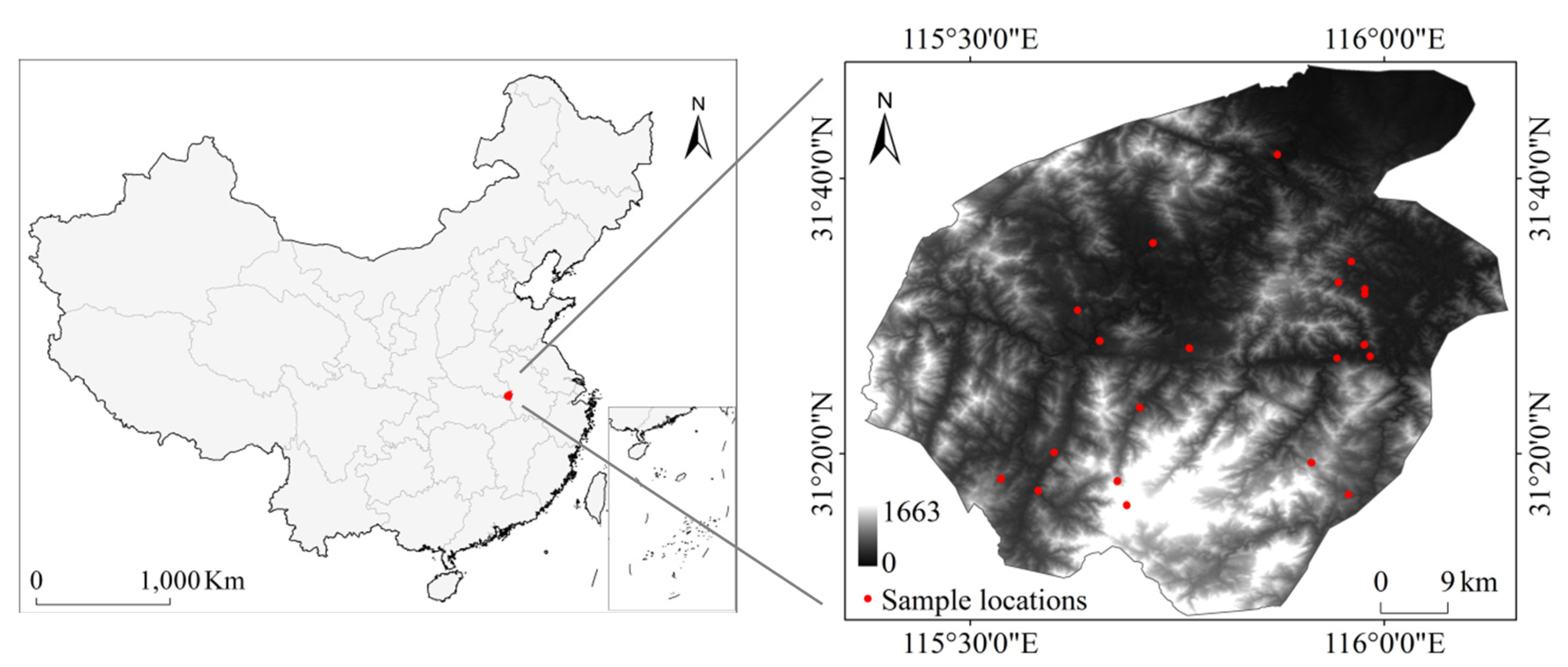
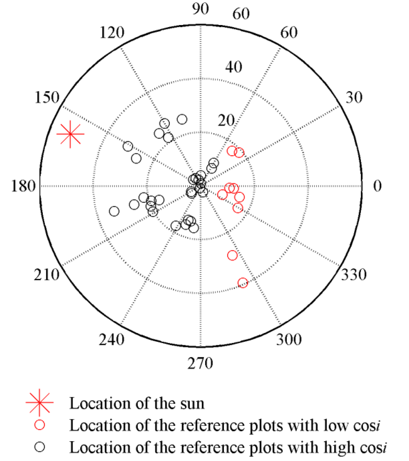
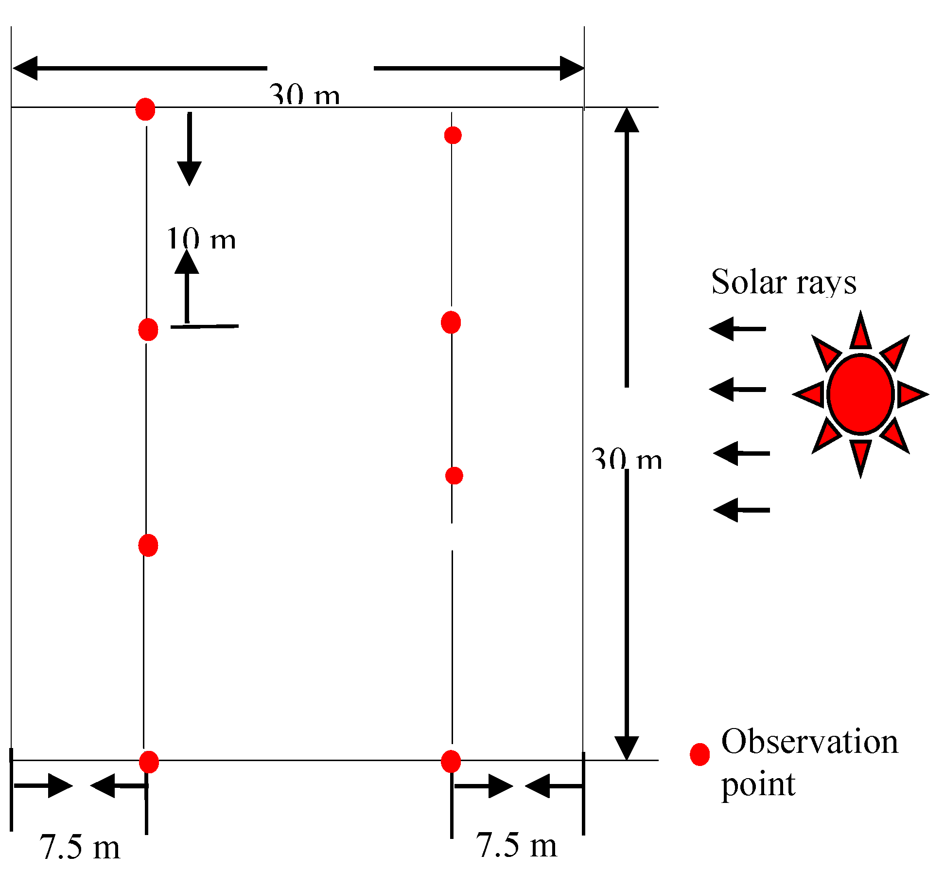
2.1. Study Area and Field Measurements

| Reference Plots | Reference Plots | ||||||||
|---|---|---|---|---|---|---|---|---|---|
| ID | Elevation | Slope | Aspect | Cosi | ID | Elevation | Slope | Aspect | Cosi |
| 1 | 149 | 39.26 | 293.43 | 0.1237 | 22 | 149 | 17.46 | 238 | 0.6295 |
| 2 | 124 | 28.4 | 294.59 | 0.2707 | 23 | 117 | 3.81 | 90 | 0.6331 |
| 3 | 25 | 15.95 | 329.32 | 0.3776 | 24 | 117 | 3.81 | 90 | 0.6331 |
| 4 | 38 | 15.05 | 343.81 | 0.3902 | 25 | 162 | 2.26 | 108.44 | 0.6347 |
| 5 | 195 | 12.26 | 355.6 | 0.4412 | 26 | 136 | 4.39 | 220.6 | 0.6414 |
| 6 | 68 | 18.91 | 41.05 | 0.4650 | 27 | 136 | 4.17 | 210.96 | 0.6483 |
| 7 | 22 | 10.64 | 356.18 | 0.4659 | 28 | 165 | 3.44 | 123.69 | 0.6529 |
| 8 | 27 | 8.71 | 337.62 | 0.4887 | 29 | 27 | 3.72 | 140.19 | 0.6624 |
| 9 | 59 | 17.37 | 48.24 | 0.5064 | 30 | 57 | 20.26 | 208.3 | 0.7528 |
| 10 | 158 | 15.8 | 260.68 | 0.5463 | 31 | 131 | 16.44 | 198.95 | 0.7594 |
| 11 | 151 | 13.64 | 254.06 | 0.5795 | 32 | 168 | 25.65 | 105.6 | 0.7611 |
| 12 | 66 | 9.78 | 60.89 | 0.5889 | 33 | 40 | 20.02 | 202.17 | 0.7727 |
| 13 | 51 | 15.48 | 248.84 | 0.5912 | 34 | 53 | 19.19 | 196.7 | 0.7842 |
| 14 | 56 | 7.58 | 58.09 | 0.5913 | 35 | 106 | 21.62 | 123.86 | 0.8112 |
| 15 | 137 | 13.59 | 250 | 0.5927 | 36 | 115 | 21.58 | 191.55 | 0.8146 |
| 16 | 163 | 2.49 | 287.18 | 0.5931 | 37 | 62 | 25.65 | 195.6 | 0.8262 |
| 17 | 146 | 0.75 | 251.57 | 0.6145 | 38 | 34 | 26.84 | 120.16 | 0.8286 |
| 18 | 146 | 0.75 | 251.57 | 0.6145 | 39 | 69 | 24.83 | 128.42 | 0.8451 |
| 19 | 146 | 0.75 | 251.57 | 0.6145 | 40 | 98 | 33.6 | 196.39 | 0.8560 |
| 20 | 146 | 0.75 | 251.57 | 0.6145 | 41 | 121 | 26.06 | 156.93 | 0.8988 |
| 21 | 7 | 0.95 | 90 | 0.6198 | 42 | 145 | 30.82 | 151.65 | 0.9293 |
| Variables | Mean | Std. dev. | Min. | Max. |
|---|---|---|---|---|
| fAPAR | 0.7944 | 0.1035 | 0.5754 | 0.9370 |
| LAI | 3.54 | 1.59 | 1.09 | 6.37 |
| SD [ha−1] | 1695 | 1767 | 244 | 5155 |
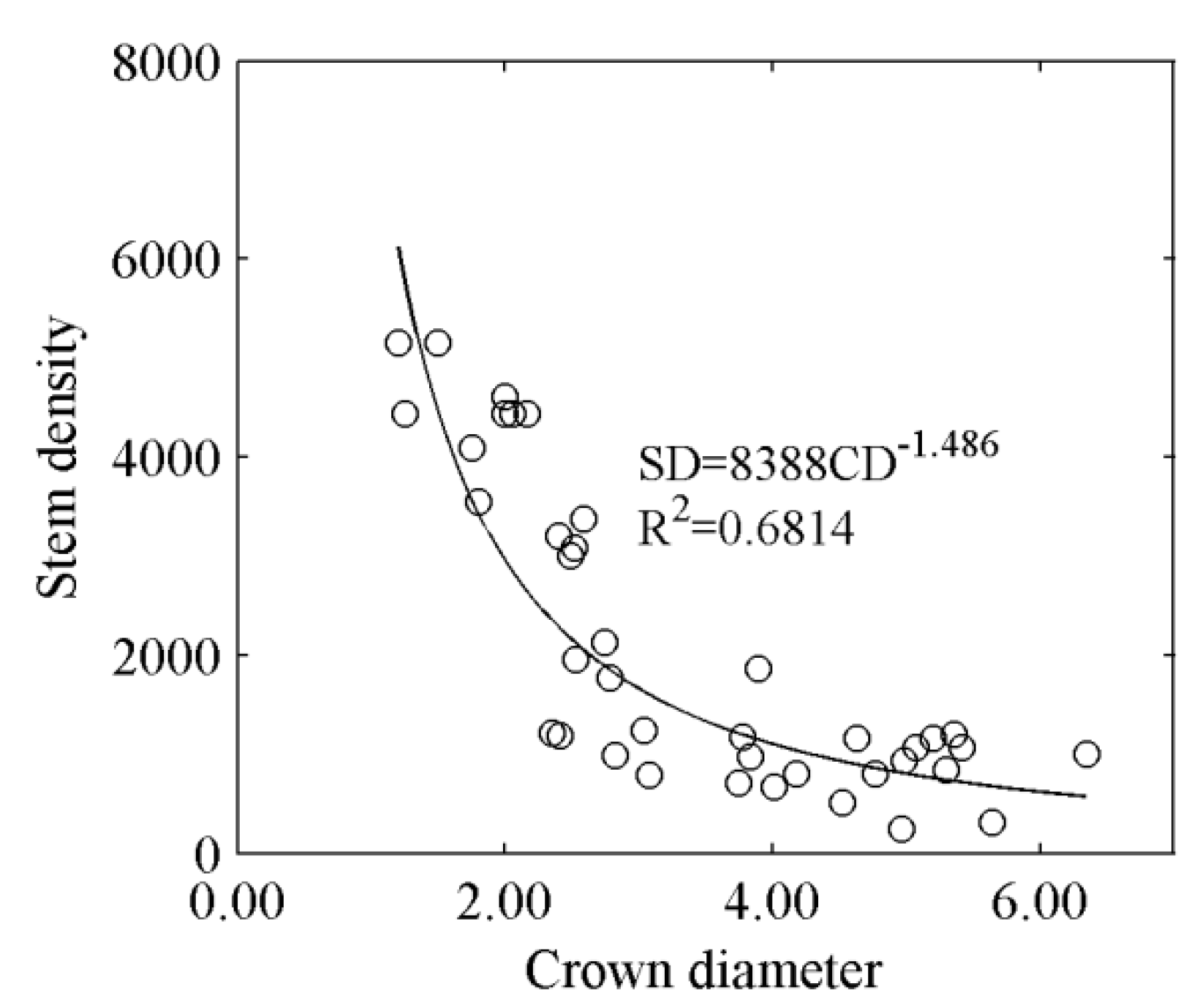
| CD[m] | 5.16 | 1.46 | 1.20 | 5.64 |
| H [m] | 10.19 | 3.05 | 5.50 | 13.31 |
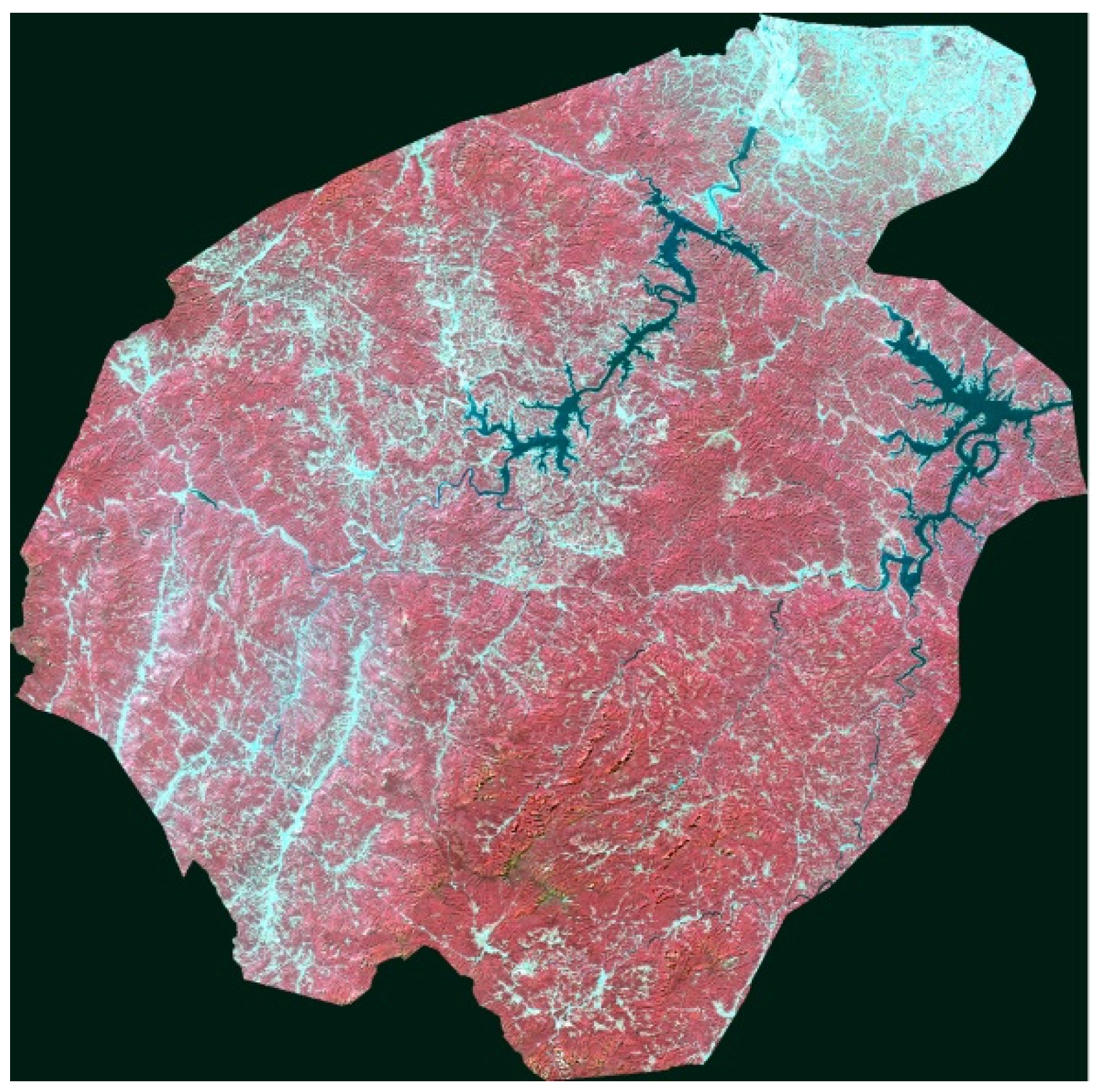
2.2. Image Data and Image Pre-Processing

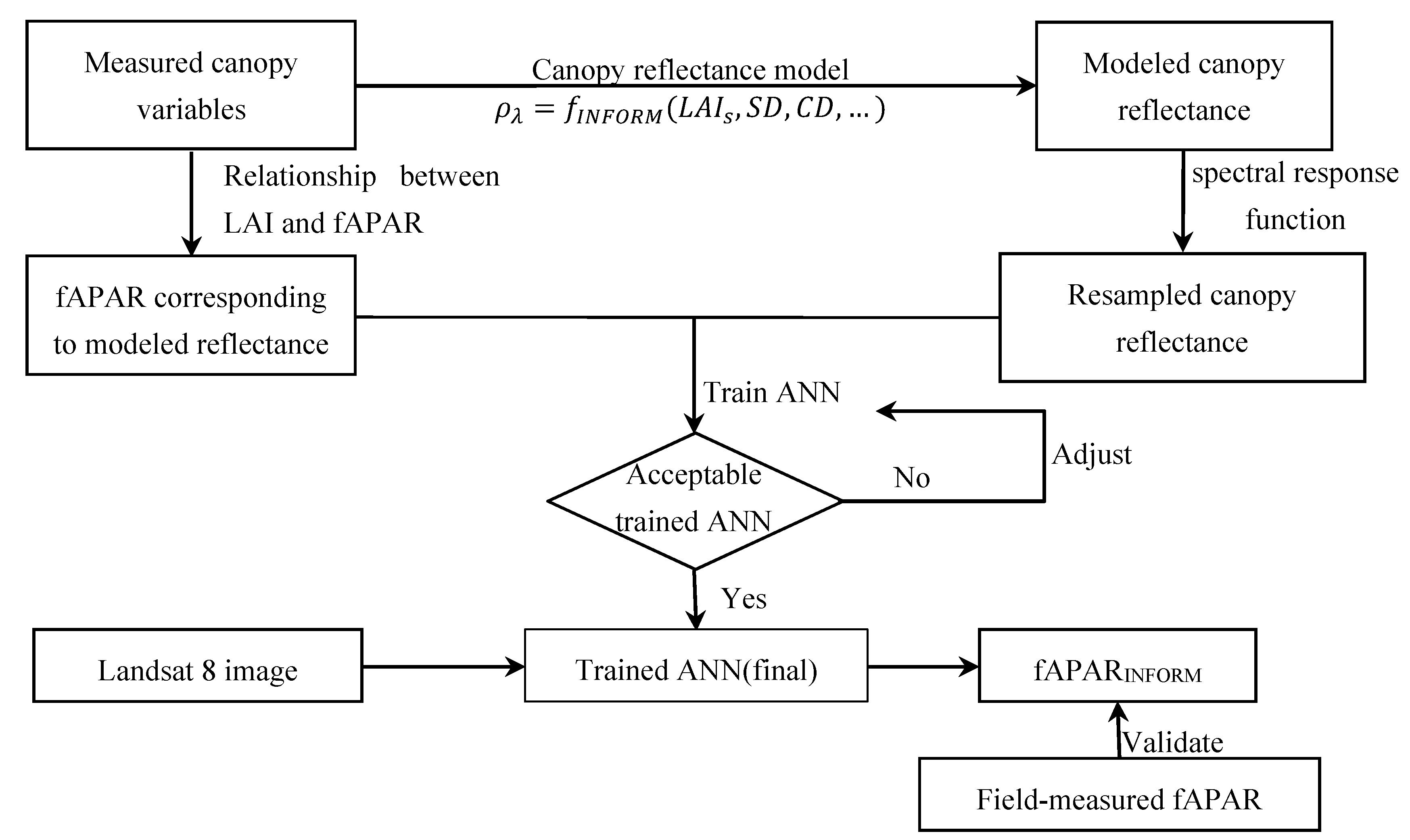
3. Method
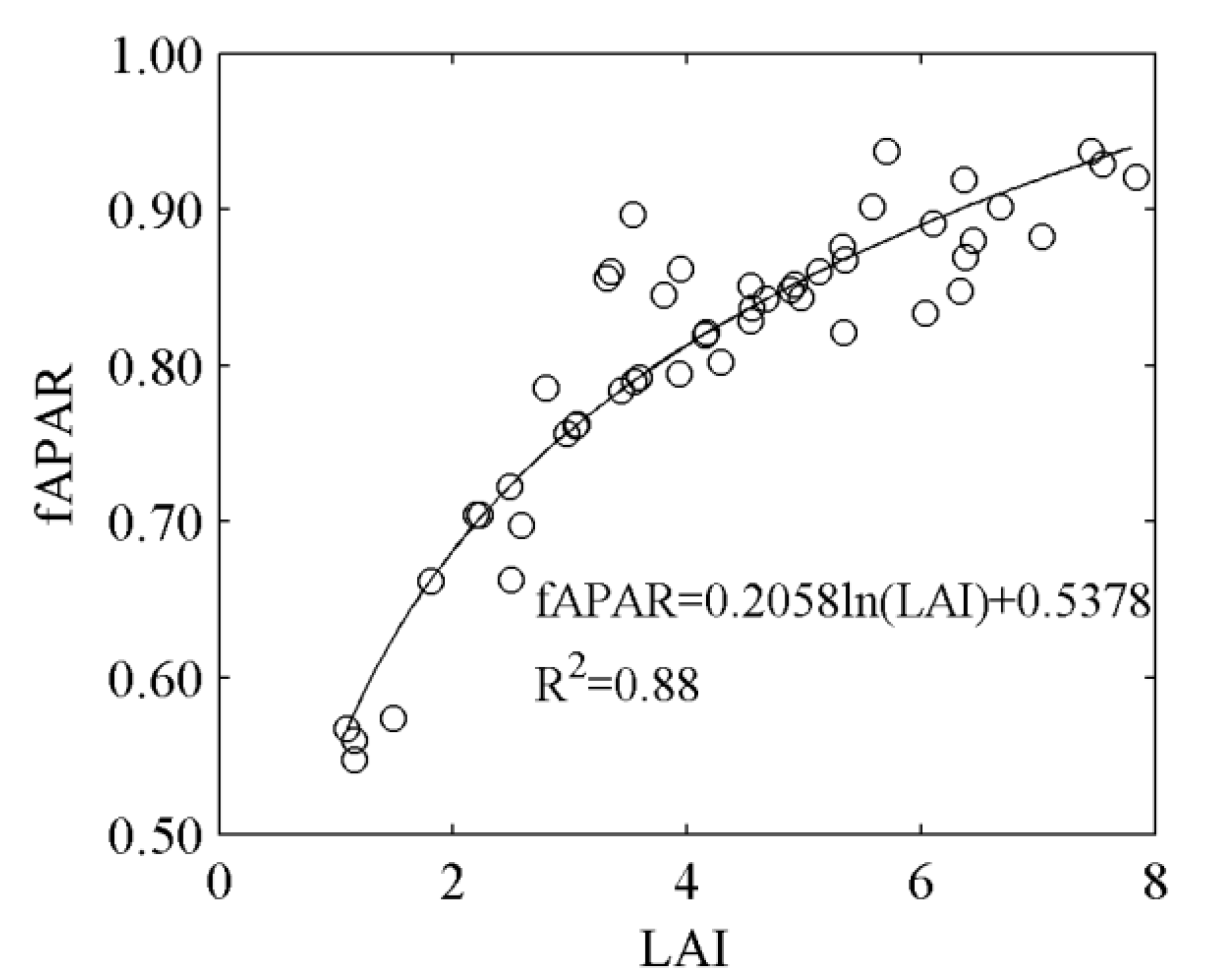
- (a)
- establishing an empirical relationships between field measured LAI and in situ fAPAR,
- (b)
- modeling visible and near-infrared bi-directional spectral reflectance of forest canopies with variable structure, leaf bio-chemistry and canopy background reflectance using INFORM,
- (c)
- using INFORM to generate a synthetic fAPAR dataset through application of the empirical relationship between LAI and fAPAR to the LAI values used as input to the synthetic reflectance data base,
- (d)
- determining the predictive relationship between spectral reflectance and fAPAR of the synthetic data base based on back-propagation (BP) neural networks, and
- (e)
- applying the trained ANN to remote sensing data and analyzing the simulated results.
3.1. INFORM
| Synthetic Variables | Designation | Corresponding Real Variables |
|---|---|---|
| Reflectance at infinite crown depth | RC | LAIinf, ALA, τleaf, ρleaf, ρsoil, θo, θs, ψ, skyl, hot |
| Background reflectance | RG | LAIU, ALAU, τleaf, ρleaf, ρsoil, θo, θs, ψ, skyl, hot |
| Leaf transmittance | τleaf | N, Cab, Cm, Cw |
| Leaf reflectance | ρleaf | N, Cab, Cm, Cw |
| Crown factor | C | To, Ts, co, cs |
| Ground factor | G | co, cs, ρ |
| Average crown transmittance in observation direction | To | LAI, ALA, τleaf, ρleaf, θo, ψ, skyl, hot |
| Average crown transmittance in the sun direction | Ts | LAI, ALA, τleaf, ρleaf, θs, ψ, skyl, hot |
| Ground coverage by crowns in observation direction | co | SD, CD, θo |
| Ground coverage by shadow in sun direction | cs | SD, CD, θS |
| Correlation between co and cs | ρ | CD, H, g |
| Geometrical factor | g | θo, θs, ψ |
| Variable | Designation | Unit | Value |
|---|---|---|---|
| Sun zenith angle | θs | deg | 42.6133 |
| Observation zenith angle | θo | deg | 0 |
| Azimuth angle | Ψ | deg | 180 |
| Fraction of diffuse radiation | skyl | fraction | 0.1 |
| Hot spot parameter | hot | ratio | 1.4 |
| Average leaf angle of tree canopy | ALA | deg | 55 |
| Leaf area index at infinite crown depth | LAIinf | m2·m−2 | 15 |
| Leaf area index of understory | LAIU | m2·m−2 | 0.5 |
| Average leaf angle of understory | ALAU | deg | 45 |
| Chlorophyll content(a+b) | Cab | µg·cm−2 | 44 |
| Cellulose and lignin content | Cm | g·cm−2 | 0.003493 |
| Equivalent water thickness | Cw | g·cm−2 | 0.009 |
| Mesophyll structure parameter | N | / | 1.7 |
3.2. Training the Artificial Neural Network
3.2.1. Generating the Training Database

3.2.2. Establishing the Network Architecture and Training
4. Results and Discussion
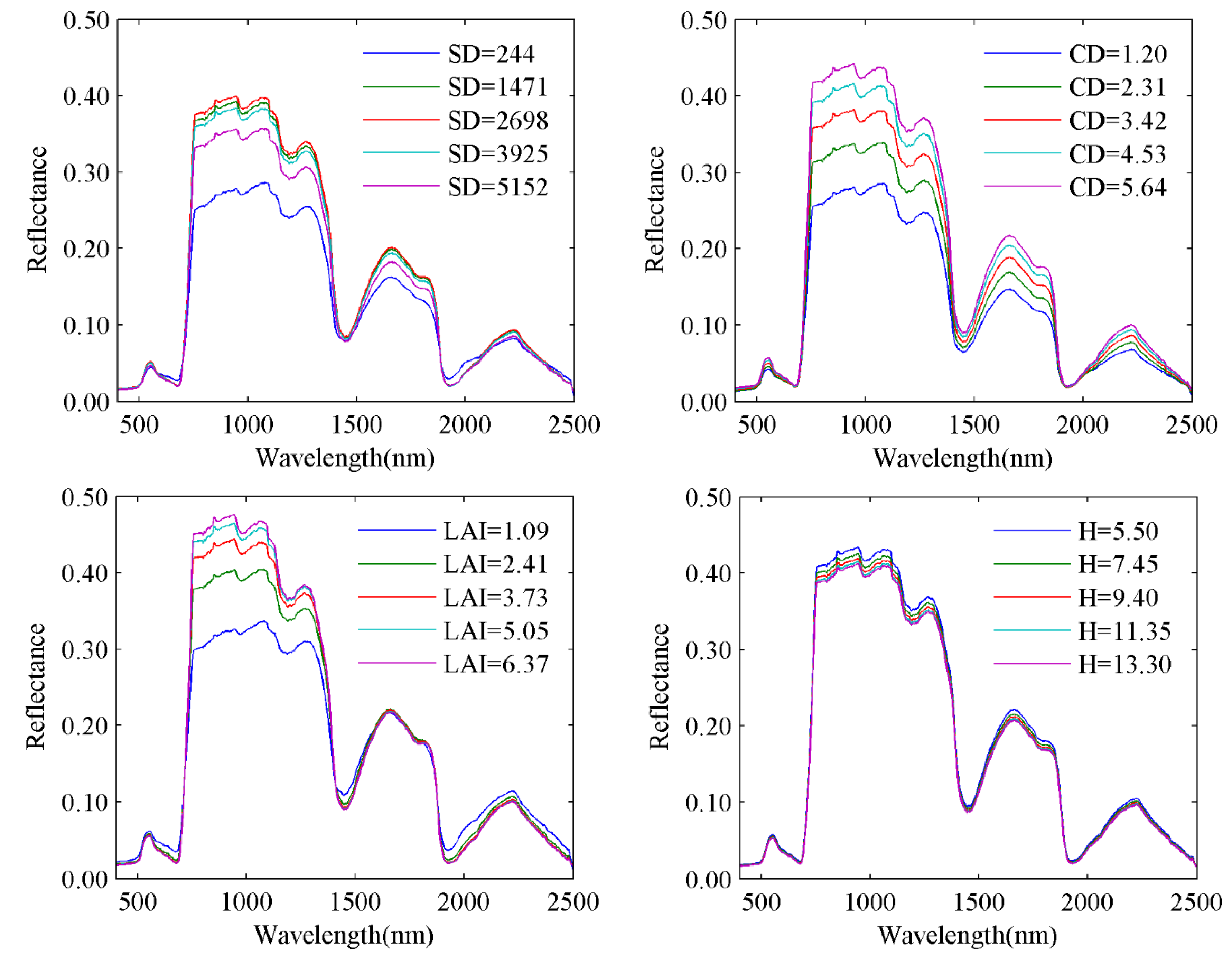
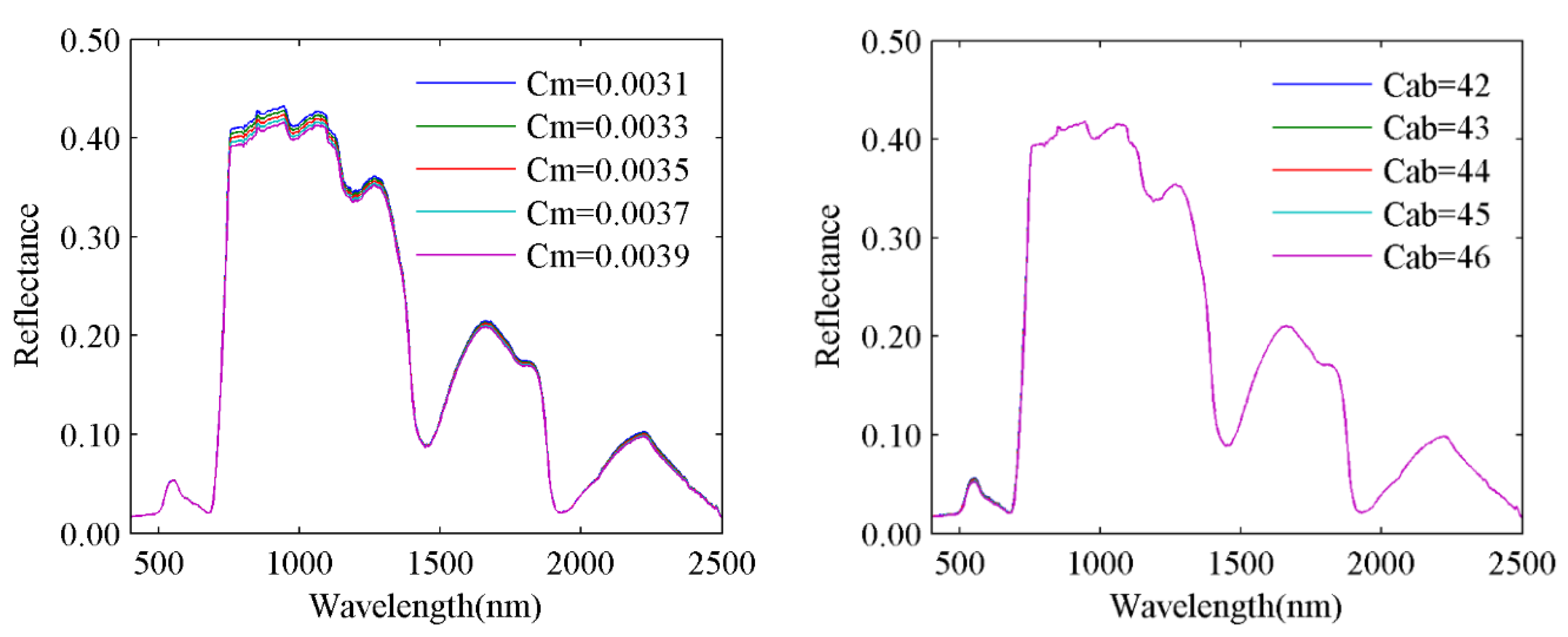
4.1. Sensitivity Analysis of INFORM Parameters
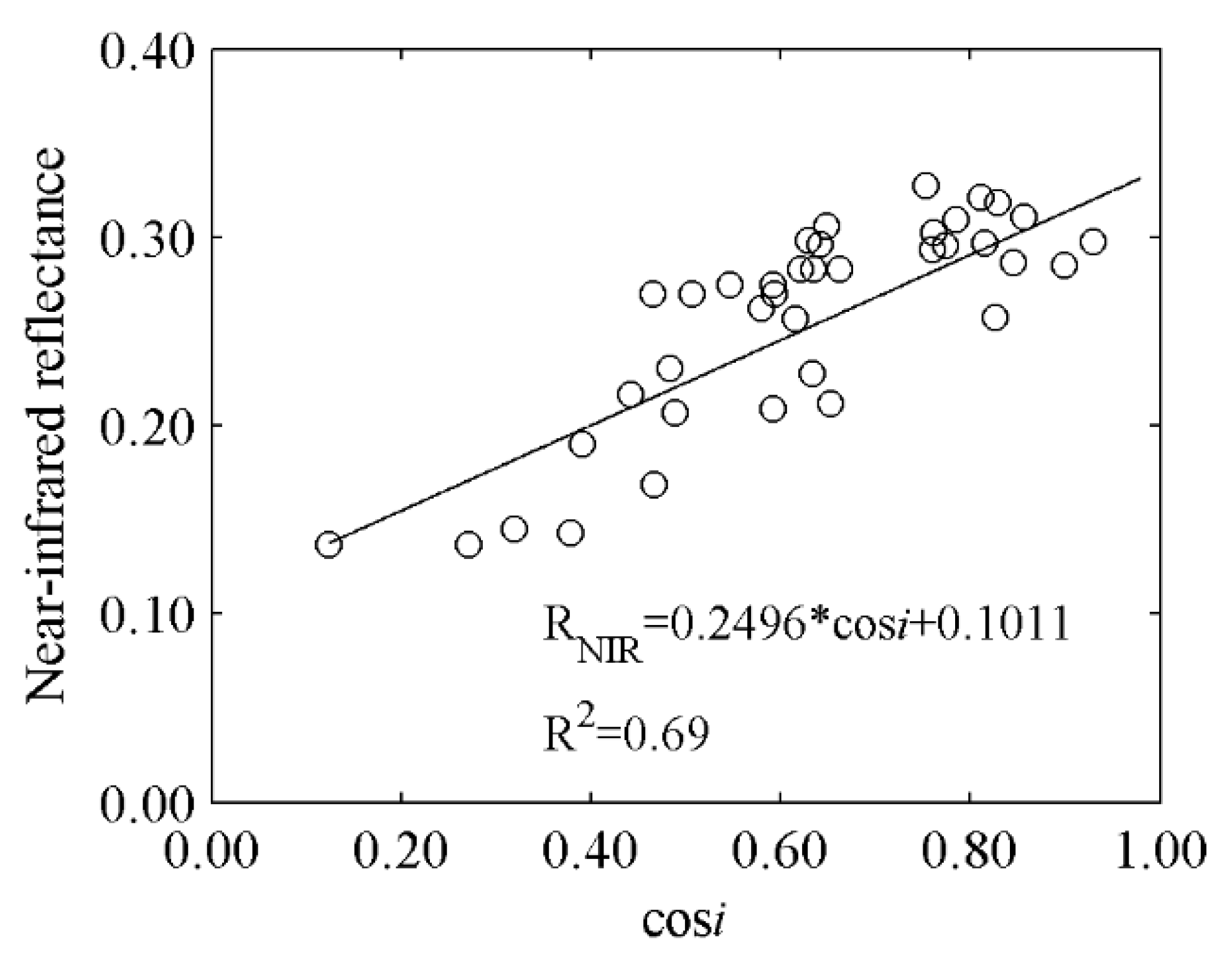
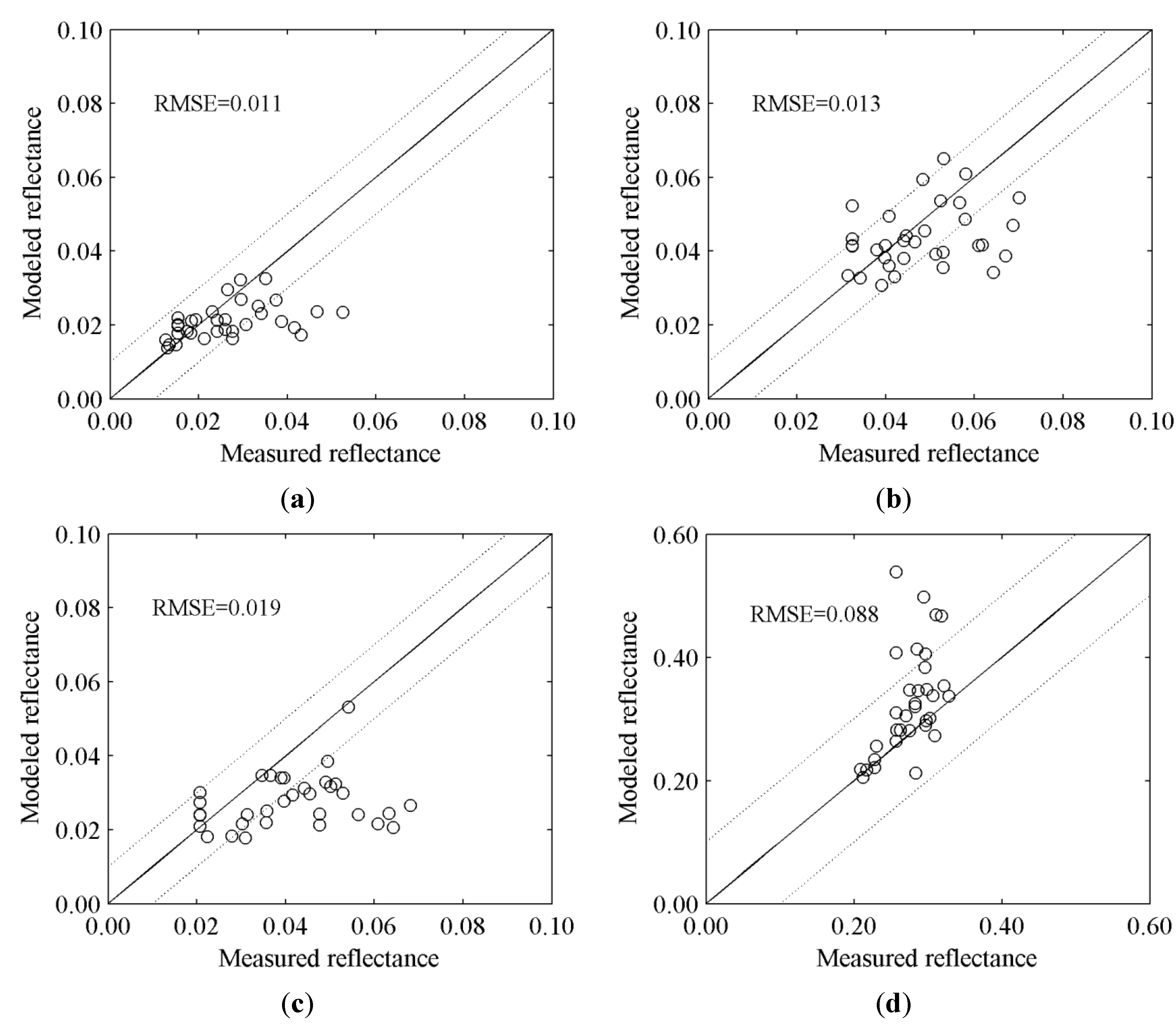
4.2. Validation of the Modelled Canopy Reflectance
| “Steep” Terrain (LOw cosi) | “Normal” Terrain (High cosi) | |||
|---|---|---|---|---|
| n | RMSE | n | RMSE | |
| Blue | 9 | 0.013 | 33 | 0.011 |
| Green | 9 | 0.019 | 33 | 0.013 |
| Red | 9 | 0.021 | 33 | 0.019 |
| nIR | 9 | 0.200 | 33 | 0.088 |
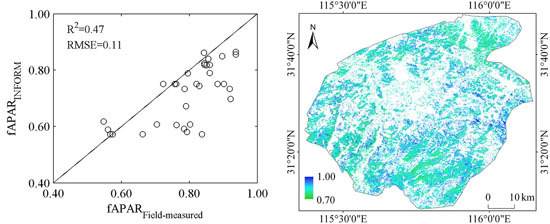
4.3. Validation of fAPAR Inversion Results
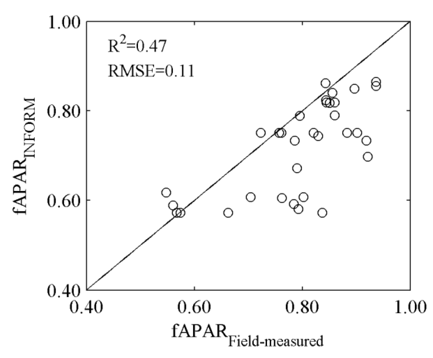
| “Steep” Terrain (Low cosi) | “Normal” Terrain (High cosi) | ||||
|---|---|---|---|---|---|
| n | RMSE | R2 | n | RMSE | R2 |
| 9 | 0.16 | 0.03 | 33 | 0.11 | 0.47 |
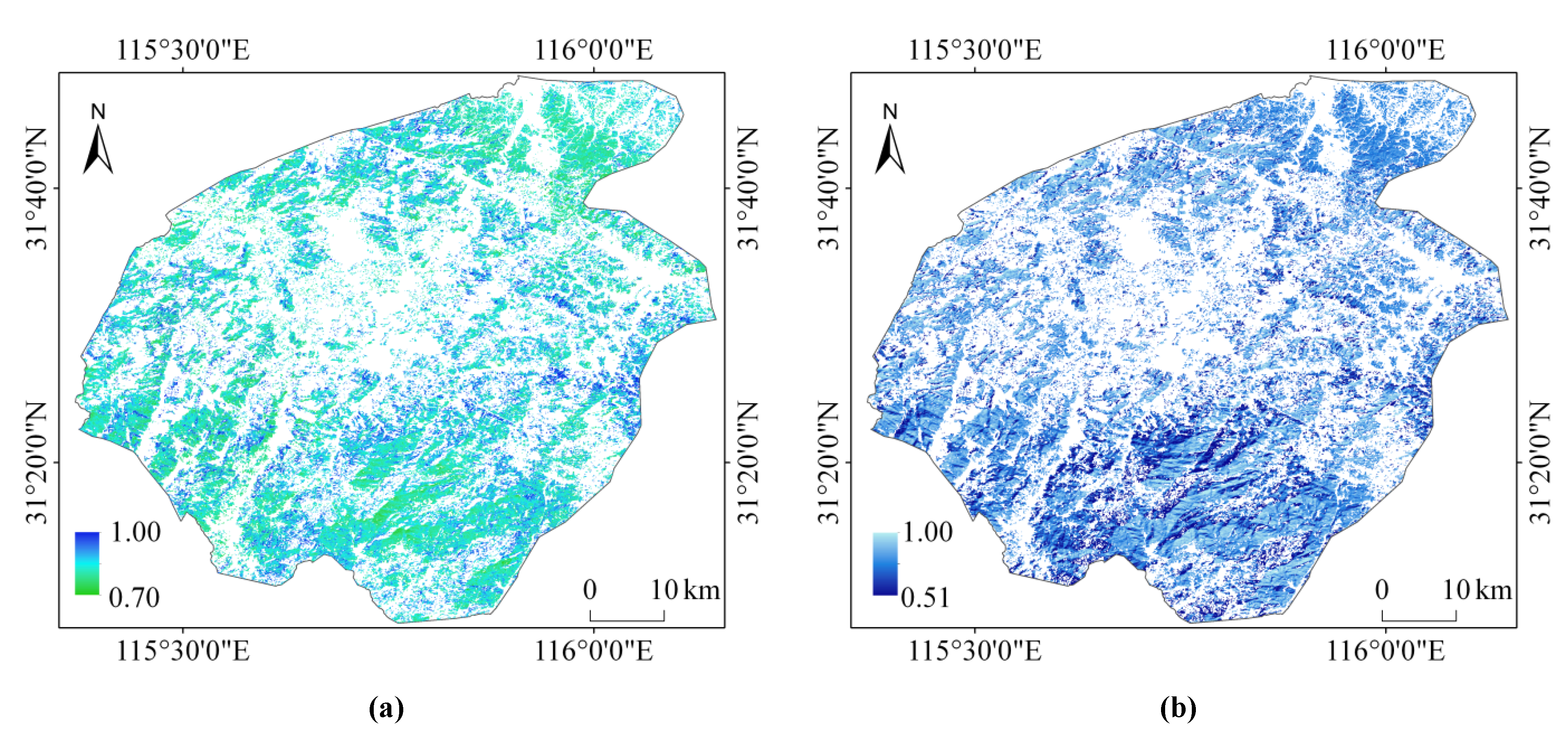
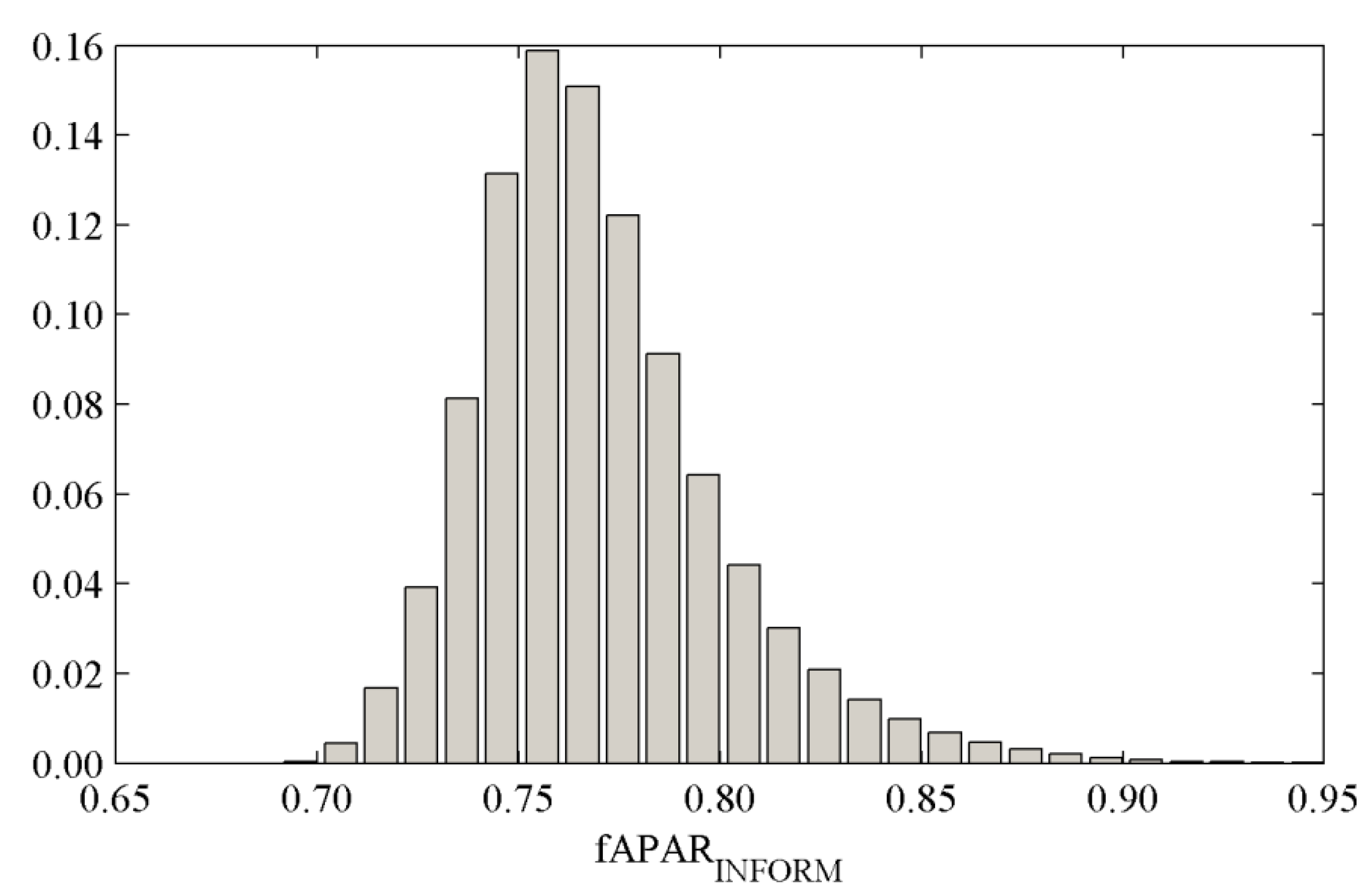
4.4. Estimation of Forest fAPAR in the Study Area
5. Conclusions
- (1)
- INFORM seems moderately well suited for modeling the bi-directional spectral reflectance of forest canopies in the visible and near-infrared bands as a function of structural and bio-chemical forest characteristics. The parameters most strongly influencing the simulated reflectances of the model are LAI, crown diameter, and stem density. The modelled reflectance showed a consistent underestimation in red band and overestimation in near-infrared band. Probably, part of the differences could be reduced by using higher precision field measurement data. For example, in-situ leaf characteristics and other species-related factors were neglected in this study or unavailable. Obviously, being a relatively simple CRM, INFORM only captures the main factors of variability. More advanced CRMs need to be tested to reach a closer agreement between forward simulations and Landsat observations.
- (2)
- The forest fAPAR was modeled for the Dabie mountain test site by inverting INFORM through an artificial neural network approach. Results suggest that this method can successfully estimate forest fAPAR from multispectral images and achieve an acceptable accuracy with RMSE of 0.11 (14% of average) and R2 of 0.47. In further studies, efforts will be made to estimate and evaluate time series of forest fAPAR based on the method.
- (3)
- The mountainous terrain posed the biggest challenge for successful retrieval of fAPAR. The employed simple topographic C-correction method created several overcorrections and artifacts negatively influencing the fAPAR retrieval. The insufficient topographic correction already became visible when running INFORM in forward mode (e.g., with field measured canopy characteristics entered into the CRM). In doing so, it was noted that the simulated canopy reflectance spectra strongly deviated from the observed (Landsat-8) spectral profiles.
Acknowledgments
Author Contributions
Conflicts of Interest
References
- Monteith, J.L.; Moss, C.J. Climate and efficiency of crop production in Britan. Philos. Trans. R. Soc. Lond. Ser. B 1977, 281, 277–294. [Google Scholar] [CrossRef]
- Goel, N.S.; Strebel, D.E. Inversion of vegetation canopy reflectance models for estimating agronomic variables.1. Problem definition and initial results using the suits model. Remote Sens. Environ. 1983, 13, 487–507. [Google Scholar] [CrossRef]
- Myneni, R.B.; Williams, D.L. On the relationship between FAPAR and NDVI. Remote Sens. Environ. 1994, 49, 200–211. [Google Scholar] [CrossRef]
- Steinberg, D.C.; Goetz, S.J.; Hyer, E.J. Validation of MODIS F-PAR products in boreal forests of Alaska. IEEE Trans. Geosci. Remote Sens. 2006, 44, 1818–1828. [Google Scholar] [CrossRef]
- Verger, A.; Baret, F.; Camacho, F. Optimal modalities for radiative transfer-neural network estimation of canopy biophysical characteristics: Evaluation over an agricultural area with CHRIS/PROBA observations. Remote Sens. Environ. 2011, 115, 415–426. [Google Scholar] [CrossRef]
- Iaquinta, J.; Pinty, B.; Privette, J.L. Inversion of a physically based bidirectional reflectance model of vegetation. IEEE Trans. Geosci. Remote Sens. 1997, 35, 687–698. [Google Scholar] [CrossRef]
- Vanonckelen, S.; Lhermitte, S.; Balthazar, V.; Van Rompaey, A. Performance of atmospheric and topographic correction methods on Landsat imagery in mountain areas. Int. J. Remote Sens. 2014, 35, 4952–4972. [Google Scholar] [CrossRef]
- Shepherd, J.D.; Dymond, J.R. Correcting satellite imagery for the variance of reflectance and illumination with topography. Int. J. Remote Sens. 2003, 24, 3503–3514. [Google Scholar] [CrossRef]
- Peddle, D.R.; Teillet, P.M.; Wulder, M.A. Radiometric image processing. In Remote Sensing of Forest Environments: Concepts and Case Studies; Springer: Berlin, Germany, 2003; pp. 181–208. [Google Scholar]
- Suits, G.H. The calculation of directional reflectance of a vegetation canopy. Remote Sens. Environ. 1972, 2, 117–125. [Google Scholar] [CrossRef]
- Verhoef, W. Light-scattering by leaf layers with application to canopy reflectance modeling: The SAIL model. Remote Sens. Environ 1984, 16, 125–141. [Google Scholar] [CrossRef]
- Asner, G.P.; Hicke, J.A.; Lobel, D.B. Per-pixel analysis of forest structure—Vegetation indices, spectral mixture analysis and canopy reflectance modeling. In Remote Sensing of Forest Environments: Concepts and Case Studies; Springer: Berlin, Germany, 2003; pp. 209–254. [Google Scholar]
- Stenberg, P.; Mottus, M.; Rautiainen, M. Modeling the Spectral Signature of Forests: Application of Remote Sensing Models to Coniferous Canopies. In Advances in Land Remote Sensing: System, Modeling, Inversion and Application; Liang, S., Ed.; Springer: Dordrecht, The Netherlands, 2008; pp. 147–171. [Google Scholar]
- Myneni, R.B.; Nemani, R.R.; Running, S.W. Estimation of global leaf area index and absorbed PAR using radiative transfer models. IEEE Trans. Geosci. Remote Sens. 1997, 35, 1380–1393. [Google Scholar] [CrossRef]
- Shen, S.S.; Badhwar, G.D.; Carnes, G. Separability of boreal forest species in the Lake Jennette area, Minnesota. Photogramm. Eng. Remote Sens. 1985, 51, 1775–1783. [Google Scholar]
- Li, X.W.; Strahler, A.H. Geometric-optical bidirectional reflectance modeling of a conifer forest canopy. IEEE Trans. Geosci. Remote Sens. 1986, 24, 906–919. [Google Scholar] [CrossRef]
- Knyazikhin, Y.; Schull, M.A.; Xu, L.; Myneni, R.B.; Samanta, A. Canopy spectral invariants. Part 1: A new concept in remote sensing of vegetation. J. Quant. Spectrosc. Radiat. Transf. 2011, 112, 727–735. [Google Scholar] [CrossRef]
- Majasalmi, T.; Rautiainen, M.; Stenberg, P. Modeled and measured FPAR in a boreal forest: Validation and application of a new model. Agric. For. Meteorol. 2014, 189, 118–124. [Google Scholar] [CrossRef]
- Manninen, T.; Stenberg, P. Simulation of the effect of snow covered forest floor on the total forest albedo. Agric. For. Meteorol. 2009, 149, 303–319. [Google Scholar] [CrossRef]
- Rautiainen, M.; Stenberg, P. Application of photon recollision probability in coniferous canopy reflectance simulations. Remote Sens. Environ. 2005, 96, 98–107. [Google Scholar] [CrossRef]
- Stenberg, P.; Lukes, P.; Rautiainen, M.; Manninen, T. A new approach for simulating forest albedo based on spectral invariants. Remote Sens. Environ. 2013, 137, 12–16. [Google Scholar] [CrossRef]
- Widlowski, J.L.; Pinty, B.; Lopatka, M.; Atzberger, C.; Buzica, D.; Chelle, M.; Disney, M.; Gerboles, M.; Gastellu-Etchegorry, J.P.; Gobron, N.; et al. The fourth radiation transfer model intercomparison (RAMI-IV): Proficiency testing of canopy reflectance models with ISO-13528. J. Geophys Res.: Atmos. 2013, 118, 6869–6890. [Google Scholar]
- Atzberger, C. Development of an invertible forest reflectance model: The infor-model. In Proceedings of the 20th Annual Symposium of the European-Association-of-Remote-Sensing-Laboratories (EARSeL), Trier, Germany, 14–16 June 2000; pp. 39–44.
- Schlerf, M.; Atzberger, C. Inversion of a forest reflectance model to estimate structural canopy variables from hyperspectral remote sensing data. Remote Sens. Environ. 2006, 100, 281–294. [Google Scholar] [CrossRef]
- Rosema, A.; Verhoef, W.; Noorbergen, H.; Borgesius, J.J. A new forest light interaction model in support of forest monitoring. Remote Sens. Environ. 1992, 42, 23–41. [Google Scholar] [CrossRef]
- Gobron, N.; Pinty, B.; Verstraete, M.; Govaerts, Y. The MERIS global vegetation index (MGVI): Description and preliminary application. Int. J. Remote Sens. 1999, 20, 1917–1927. [Google Scholar] [CrossRef]
- Dong, T.; Wu, B.; Meng, J. Study of a vegetation index based on HJ CCD data’s top-of-atmosphere reflectance and FPAR inversion. IOP Conf. Ser.: Earth Environ. Sci. 2014, 17, 012029. [Google Scholar] [CrossRef]
- Baret, F.; Hagolle, O.; Geiger, B.; Bicheron, P.; Miras, B.; Huc, M.; Berthelot, B.; Nino, F.; Weiss, M.; Samain, O.; et al. LAI, FAPAR and FCOVER cyclopes global products derived from vegetation—Part 1: Principles of the algorithm. Remote Sens. Environ. 2007, 110, 275–286. [Google Scholar] [CrossRef] [Green Version]
- Casanova, D.; Epema, G.F.; Goudriaan, J. Monitoring rice reflectance at field level for estimating biomass and LAI. Field Crop. Res. 1998, 55, 83–92. [Google Scholar] [CrossRef]
- Wiegand, C.L.; Maas, S.J.; Aase, J.K.; Hatfield, J.L.; Pinter, P.J.; Jackson, R.D.; Kanemasu, E.T.; Lapitan, R.L. Multisite analyses of spectral-biophysical data for wheat. Remote Sens. Environ. 1992, 42, 1–21. [Google Scholar] [CrossRef]
- Zhou, X.D.; Zhu, Q.J.; Wang, J.D. Interaction of PAR, relationship between FPAR and LAI in summer maize canopy. J. Nat. Resour. 2002, 17, 110–116. (In Chinese) [Google Scholar]
- Zhou, X.D.; Zhu, Q.J.; Tang, S.H.; Chen, X.; Wu, M.X. Interception of PAR and Relationship between FPAR and LAI in Summer Maize Canopy. Available online: http://www.jourlib.org/paper/1497761#.VW63OUY-1ps (accessed on 5 April 2015).
- Goel, N.S. Models of vegetation canopy reflectance and their use in estimation of biophysical parameters from reflectance data. Remote Sens. Rev. 1988, 4, 1–212. [Google Scholar] [CrossRef]
- Knyazikhin, Y.; Martonchik, J.V.; Myneni, R.B.; Diner, D.J.; Running, S.W. Synergistic algorithm for estimating vegetation canopy leaf area index and fraction of absorbed photosynthetically active radiation from MODIS and MISR data. J. Geophys. Res.-Atmos. 1998, 103, 32257–32275. [Google Scholar] [CrossRef]
- Combal, B.; Baret, F.; Weiss, M.; Trubuil, A.; Mace, D.; Pragnere, A.; Myneni, R.; Knyazikhin, Y.; Wang, L. Retrieval of canopy biophysical variables from bidirectional reflectance—using prior information to solve the ill-posed inverse problem. Remote Sens. Environ. 2003, 84, 1–15. [Google Scholar] [CrossRef]
- Bacour, C.; Baret, F.; Beal, D.; Weiss, M.; Pavageau, K. Neural network estimation of LAI, FAPAR, FCOVER and LAIXC(AB), from top of canopy MERIS reflectance data: Principles and validation. Remote Sens. Environ. 2006, 105, 313–325. [Google Scholar] [CrossRef]
- Proy, C.; Tanre, D.; Deschamps, P.Y. Evaluation of topographic effects in remotely sensed data. Remote Sens. Environ. 1989, 30, 21–32. [Google Scholar] [CrossRef]
- Meyer, P.; Itten, K.I.; Kellenberger, T.; Sandmeier, S.; Sandmeier, R. Radiometric correction of topographically induced effects on Landsat TM data in an alpine environment. ISPRS J. Photogramm. Remote Sens. 1993, 48, 17–28. [Google Scholar] [CrossRef]
- Chen, J.M.; Cihlar, J. Plant canopy gap-size analysis theory for improving optical measurements of leaf-area index. Appl. Opt. 1995, 34, 6211–6222. [Google Scholar] [CrossRef] [PubMed]
- Weiss, M.; Baret, F. Can-Eye v6.1 User Manual. Available online: http://www.docin.com/p-900325754.html (accessed on 5 April 2015).
- Chen, J.M.; Rich, P.M.; Gower, S.T.; Norman, J.M.; Plummer, S. Leaf area index of boreal forests: Theory, techniques, and measurements. J. Geophys. Res. Atmos. 1997, 102, 29429–29443. [Google Scholar] [CrossRef]
- Yang, G.J.; Liu, Q.H.; Liu, Q.; Xiao, Q.; Huang, W.J. Directional simulation of thermal infrared radiation 3D radiative transfer model of canopy. J. Infrared Millim. Waves 2010, 29, 38–44. [Google Scholar] [CrossRef]
- Teillet, P.M.; Guindon, B.; Goodenough, D.G. On the slope-aspect correction of multispectral scanner data. Can. J. Remote Sens. 1982, 8, 1537–1540. [Google Scholar] [CrossRef]
- Gu, D.; Gillespie, A. Topographic normalization of landsat tm images of forest based on subpixel sun-canopy-sensor geometry. Remote Sens. Environ. 1998, 64, 166–175. [Google Scholar] [CrossRef]
- Kuusk, A. The hot-spot effect in the leaf canopy. In Proceedings of the1991 International Geoscience and Remote Sensing Symposium, Espoo, Finland, 3–6 June 1991.
- Jacquemoud, S.; Baret, F. Prospect—A model of leaf optical properties spectra. Remote Sens. Environ. 1990, 34, 75–91. [Google Scholar] [CrossRef]
- Hosgood, B.; Jadquemoud, S.; Reoli, G.; Verdebout, J.; Pedrini, A.; Schmuck, G. The JRC Leaf Optical Properties Experiment (Lopex'93). Available online: http://www.gfsoso.net/?q=The+JRC+leaf+optical+properties+experiment+%28lopex%2793%29 (accessed on 5 April 2015).
- Kimes, D.S.; Nelson, R.F. Attributes of neural networks for extracting continuous vegetation variables from optical and radar measurements. Int. J. Remote Sens. 1998, 19, 2639–2663. [Google Scholar] [CrossRef]
- Baret, F.; Guyot, G. Potentials and limits of vegetation indexes for LAI and APAR assessment. Remote Sens. Environ. 1991, 35, 161–173. [Google Scholar] [CrossRef]
- Atkinson, P.M.; Tatnall, A.R.L. Neural networks in remote sensing—Introduction. Int. J. Remote Sens. 1997, 18, 699–709. [Google Scholar] [CrossRef]
© 2015 by the authors; licensee MDPI, Basel, Switzerland. This article is an open access article distributed under the terms and conditions of the Creative Commons Attribution license (http://creativecommons.org/licenses/by/4.0/).
Share and Cite
Yuan, H.; Ma, R.; Atzberger, C.; Li, F.; Loiselle, S.A.; Luo, J. Estimating Forest fAPAR from Multispectral Landsat-8 Data Using the Invertible Forest Reflectance Model INFORM. Remote Sens. 2015, 7, 7425-7446. https://doi.org/10.3390/rs70607425
Yuan H, Ma R, Atzberger C, Li F, Loiselle SA, Luo J. Estimating Forest fAPAR from Multispectral Landsat-8 Data Using the Invertible Forest Reflectance Model INFORM. Remote Sensing. 2015; 7(6):7425-7446. https://doi.org/10.3390/rs70607425
Chicago/Turabian StyleYuan, Huili, Ronghua Ma, Clement Atzberger, Fei Li, Steven Arthur Loiselle, and Juhua Luo. 2015. "Estimating Forest fAPAR from Multispectral Landsat-8 Data Using the Invertible Forest Reflectance Model INFORM" Remote Sensing 7, no. 6: 7425-7446. https://doi.org/10.3390/rs70607425