This section provides the basis of the retrieval, first by explaining the general principles and then the two variants of the technique used later in the study.
4.1. General Method for Effective Radius Retrieval
As stated above, C6 MYD06 contains cloud emissivity (
ec) for the 8.5, 11 and 12 μm MODIS channels (bands 29, 31 and 32).
ec is computed in the MYD06 cloud height algorithm using the following equation
where
I is the observed radiance,
Iclr is the computed clear-sky radiance,
Iac is the radiance component coming from the atmosphere above the cloud,
tac is the transmission along the path above the cloud and B(T
c) is the Planck emission computed at the cloud temperature (T
c). The clear-sky radiative transfer model used in the MYD06 processing is the PFAAST model [
13]. The MYD06 CO
2 slicing cloud-top pressure algorithm assumes the clouds to be isothermal, non-scattering layers and does not account for multiple cloud layers [
2]. Ratios between different pairs of CO
2 absorption channels are first used to retrieve cloud-top pressure; cloud temperature is derived subsequently by comparing cloud pressure with the National Center for Environmental Prediction Global Data Assimilation System [
14] model profile for upper level clouds.
As described by Parol
et al. [
15], cloud emissivity at two different spectral bands (
x,
y) can be used to compute ratios of absorption optical depths (
β) as follows:
As further described in Parol
et al. [
15],
β values can be approximated very accurately based solely on the single scattering properties of
ωo,
g, and
Qe using the following relationship:
The spectral variation of the single scattering properties for solid bullet rosettes from 8 to 13 μm is shown in
Figure 2. The
β values shown in
Figure 2 are referenced to 11 μm. Note the significant spectral variation of the properties through the 8–12 μm IR window region.
Figure 2.
Spectral variation of the single scattering properties for solid bullet rosettes over the spectral range of MODIS bands 29, 31 and 32, assuming an effective particle size of 30 μm. The grey regions show the spectral response functions for bands 29, 31 and 32.
Figure 2.
Spectral variation of the single scattering properties for solid bullet rosettes over the spectral range of MODIS bands 29, 31 and 32, assuming an effective particle size of 30 μm. The grey regions show the spectral response functions for bands 29, 31 and 32.
For the ice cloud bulk scattering properties, the values of the single scattering properties in the ice particle database are integrated over C6 MYD06 size distribution and over the spectral response functions shown in
Figure 2. Though roughening has little impact at IR wavelengths, only the severely roughened crystals were used to be consistent with the MODIS C6 optical property retrievals.
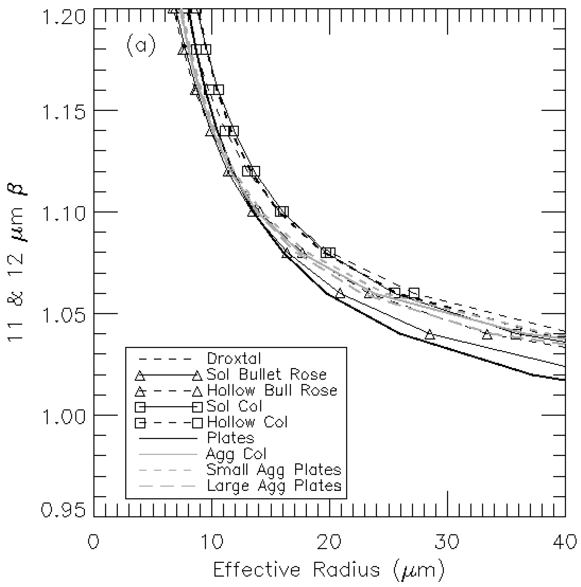
Figure 3 shows the variation in the 11–12 μm
β value as a function of effective radius for each of the nine habits.
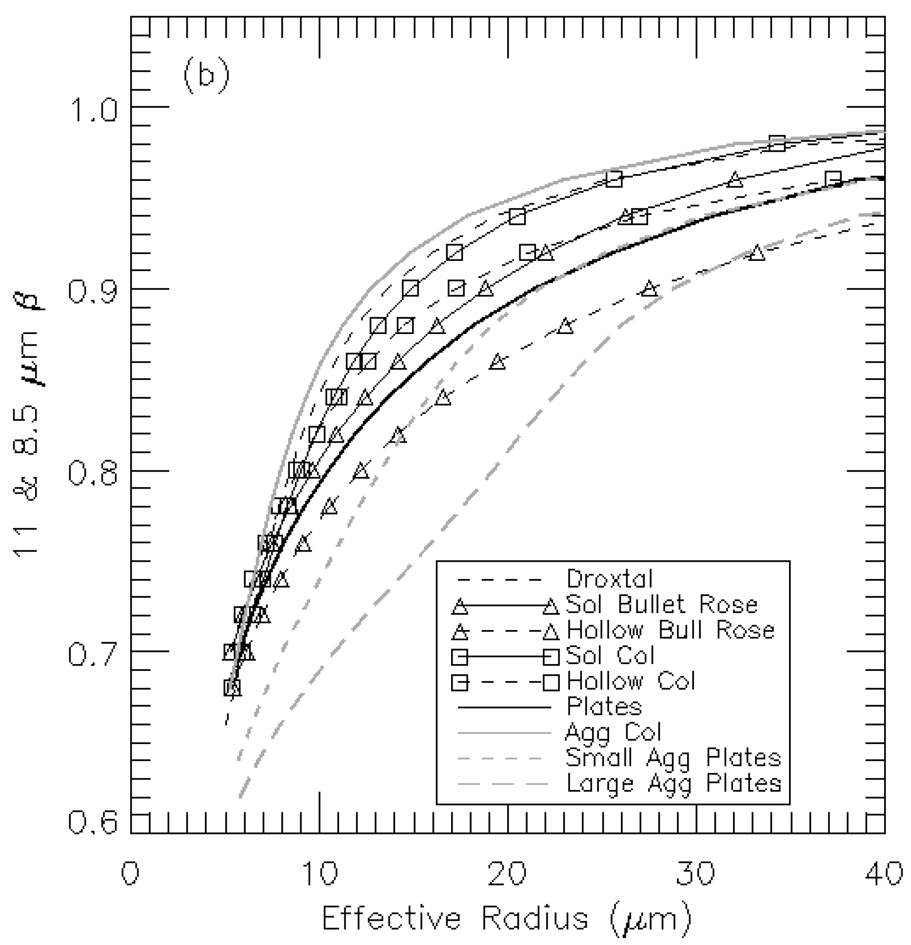
Figure 4 shows the same plot for the 11–8.5 μm
β values.
Figure 3.
Variation of β computed using the MODIS 11 μm and 12 μm channels as a function of effective radius for the nine habits in the spectral library.
Figure 3.
Variation of β computed using the MODIS 11 μm and 12 μm channels as a function of effective radius for the nine habits in the spectral library.
Based on the
β values, the retrieval of particle size is straightforward. The three values of
ec generate two values of
β. As
Figure 3 and
Figure 4 show, the relationship between each
β value and effective radius (
re) is monotonic and two values of
β generate two values of
re. In this technique, the final effective radius value is the average of the individual effective radii deduced from the 11–12 μm
β and the 11–8.5 μm
β.
Figure 4.
Variation of β computed using the MODIS 11 μm and 8.5 μm channels as a function of effective radius for the nine habits in the spectral library.
Figure 4.
Variation of β computed using the MODIS 11 μm and 8.5 μm channels as a function of effective radius for the nine habits in the spectral library.
4.2. General Method for Optical Depth Retrieval
The next step in this analysis is the estimation of the cirrus cloud optical depth (
τvis), which can be derived after effective particle size is retrieved. Based solely on the cloud emissivity (
ec), one can estimate the absorption optical depth (
τabs) using the following relationship:
where
μ is the cosine of the viewing zenith angle. Evoking the scaling approximations of van de Hulst [
16] allows us to estimate the full optical depth at the IR wavelength by the following relationship:
If we assume the extinction efficiency at visible wavelengths is approximately 2, we can derive the full visible wavelength using this relationship
At this point it is worth exploring the veracity of the scattering approximations using explicit radiative transfer calculations. The radiative transfer calculations were performed using an adding-doubling model to simulate a single layer isothermal cloud above a black-body surface. All atmospheric effects were ignored. The input to the model was the optical depth and effective particle radius. The model computed top-of-atmosphere radiances at 8.5, 11 and 12 μm. Cloud emissivities were then computed using Equation (1) and the values of
β were computed using Equation (2).
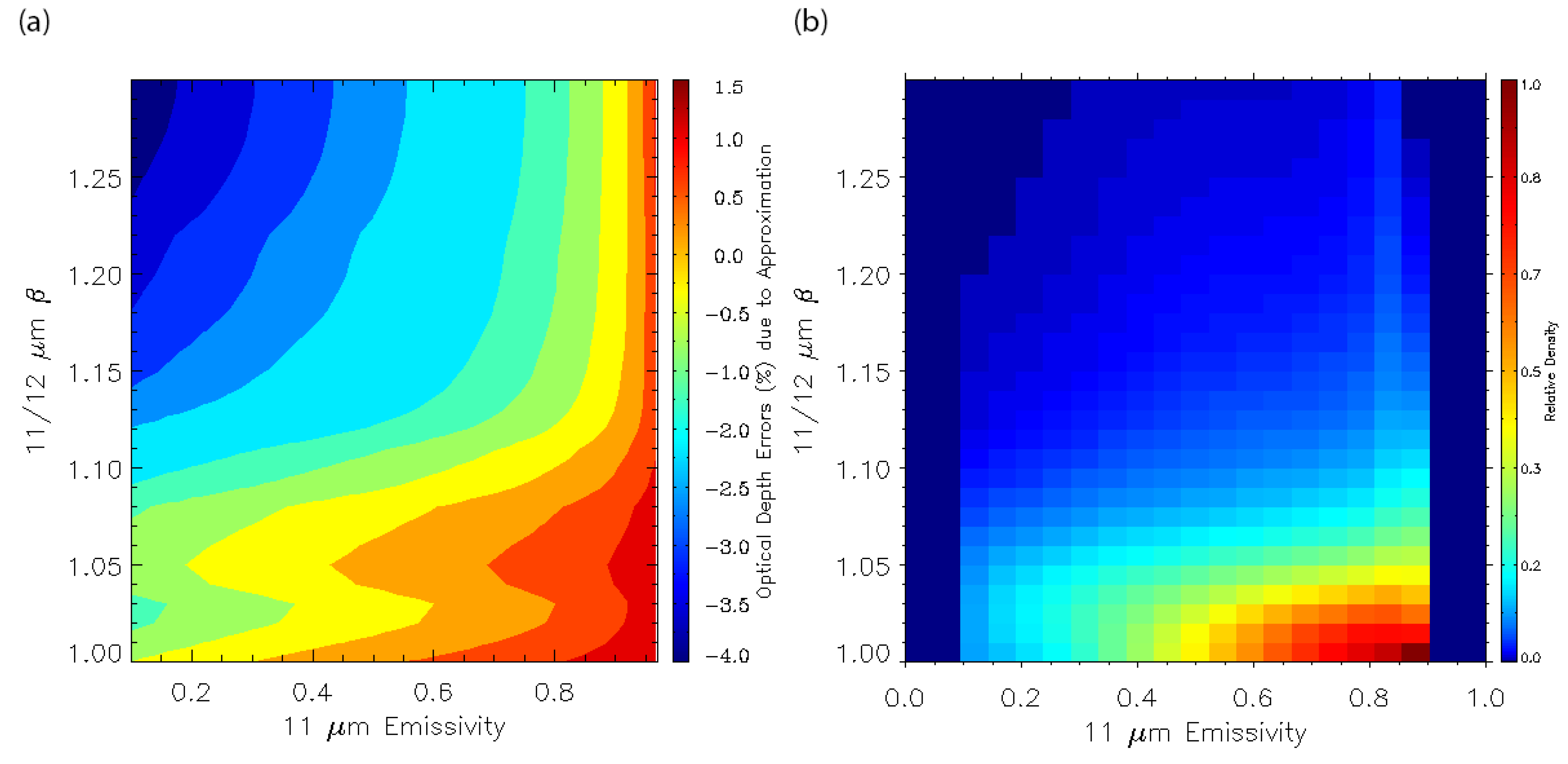
Figure 5a shows the relative errors in optical depth caused by using Equation (3) as a function of the 11 μm
ec and the 11–12 μm
β value. This figure shows the approximation for computing the full optical depth from the absorption depth and the single scattering properties is accurate to within 1% for most of the
β and
ec values. Only for small values of
ec and large values of
β do the errors exceed 3%. Higher 11–12 μm
β values correspond to smaller particle sizes where scattering plays a larger role in the total extinction process. In
Figure 5b a density plot using MODIS data is plotted, which demonstrates that data mostly concentrate when emissivity is large and 11–12 μm
β is small. Therefore, retrieval errors are expected to be small using the approximations in Equation (3).
4.3. C6 Habit
As stated earlier, we employed two variants of this technique. The first was to use a microphysical model that is consistent with that used in C6 MYD06 solar channel retrievals. The ice cloud optical property model employed for MODIS C6 is different from that assumed for earlier C5 products. The model for C6 assumes a distribution of severely roughened aggregate columns. The model for C5 assumed a habit mixture, but the crystals had smooth surfaces, with the exception of the aggregate columns. Several investigations raised issues with the C5 models that led to this change for C6. The C5 MYD06 optical depth values for cirrus were significantly higher than those reported by CALIPSO/CALIOP (e.g., [
17]). While both MODIS and CALIPSO algorithms are in active changes and new versions are being released, the latter one retrieves cloud properties from lidar signal returns and are generally considered more accurate than passive satellite retrievals. The difference between the CALIPSO and MODIS C5 optical depth values was attributed to the C5 microphysical values having a large asymmetry parameter (
g) in the solar channels that resulted in an overestimation of the optical depth (
τ). The same issue was found in a comparison of MODIS C5 cloud properties to those from POLDER (POLarization and Directionality of the Earth’s Reflectances) [
18], which assumed the use of a roughened ice particle. The adoption of severe particle roughening resulted in lower values of
g, which in turn brought the optical depth/particle size values more into line with those from CALIOP [
19].
Figure 5.
(a) shows the errors in the optical depth computed using the approximate formula in Equation (3) compared to the true optical depth. Calculations are performed using an Adding/Doubling radiative transfer model and an isothermal cloud composed of solid bullet rosettes; (b) shows the distribution of emissivity and β for one day of MODIS C6 data.
In defining the models of C6, consistency with CALIPSO/CALIOP was paramount. The nine habits of Yang’s database were analyzed and the severely roughened aggregate columns were chosen due to their agreement with CALIPSO/CALIOP. Therefore the first variant of the IR technique is to use the
β curves in
Figure 3 and
Figure 4 corresponding to the aggregate columns (solid grey line).
4.4. Empirical Method
As described above, the final
re value is calculated as the mean of the two spectral values (11–12 μm and 11–8.5 μm). It is planned to run this method on the MODIS C6 data using the same habit as that used in the C6 solar reflectance retrievals. However, it was noted that the aggregate column habit did not often produce spectral
re values that agreed with each other. A choice of other habits often reduced this spectral inconsistency. Therefore, we have implemented a second variant of the technique where the results are based on the
re value from the habit that produced the highest level of IR spectral consistency. Spectral consistency is defined as the spectral
re value whose difference was either less than 20% of the mean
re value or 1 μm. For the data analyzed here, roughly 70% of the retrievals met the criteria for spectral consistency. For simplicity, all of the results that achieved spectral consistency were used to construct empirical “radiometric” models.
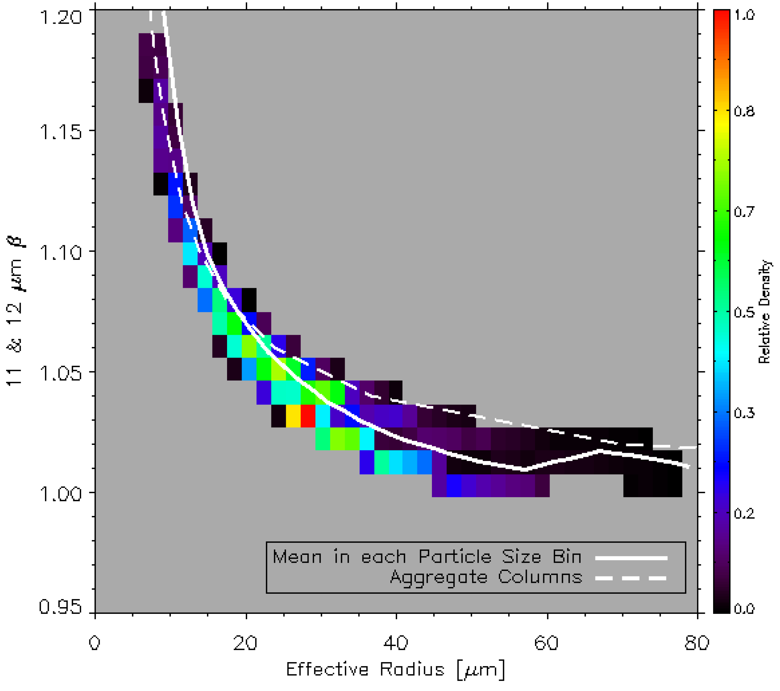
Figure 6 and
Figure 7 show the resulting empirical models for the two
β curves. Similarly, the resulting models for the other single scattering parameters (
Qe,
g,
ωo) are constructed by selecting data from the habit when the spectral consistency is achieved.
Figure 6 and
Figure 7 show the density of the retrievals with each
β and
re bin. The
β bin size is 0.01 and the
re bin size is 2 μm. The colors show the relative density of the position of spectral consistent solutions in the
β and
re space. The white solid curves plot the smoothed mean
β values within each
re bin. This smoothing has been done many times for the purpose of a smoother transition between nearby
re bins. The values shown by white solid lines therefore constitute the radiometric empirical model.
Figure 6.
Variation of the 11–12 μm β derived from the optimal habit solution as a function of effective radius. The training data are from a month of MODIS/CALIOP collocation in January 2010. Color values show the density of results within each β and effective radius bin. Solid white curves showing the variation of the mean β value after smoothing in each effective radius bin are used as the empirical model. Broken white curve shows the MODIS C6 aggregate column model.
In the radiometric empirical model, no additional habit assumption is made. Because the empirical model is based on the spectrally consistent retrievals, the spectral consistency of its
re retrievals is much superior to that with the aggregate column habit results. This method does not attempt to infer meaning in the choice of habits that result in spectral consistency, nor do we imply that the empirical model is better than the aggregate column model, but one could view this approach as suggesting that the variation in the scattering properties in Yang’s database supplies the needed range and the empirically derived curves in
Figure 6 and
Figure 7 represent the optimal radiometric model. The inference of the habit mixtures and size distributions that could produce this model is left to future studies.
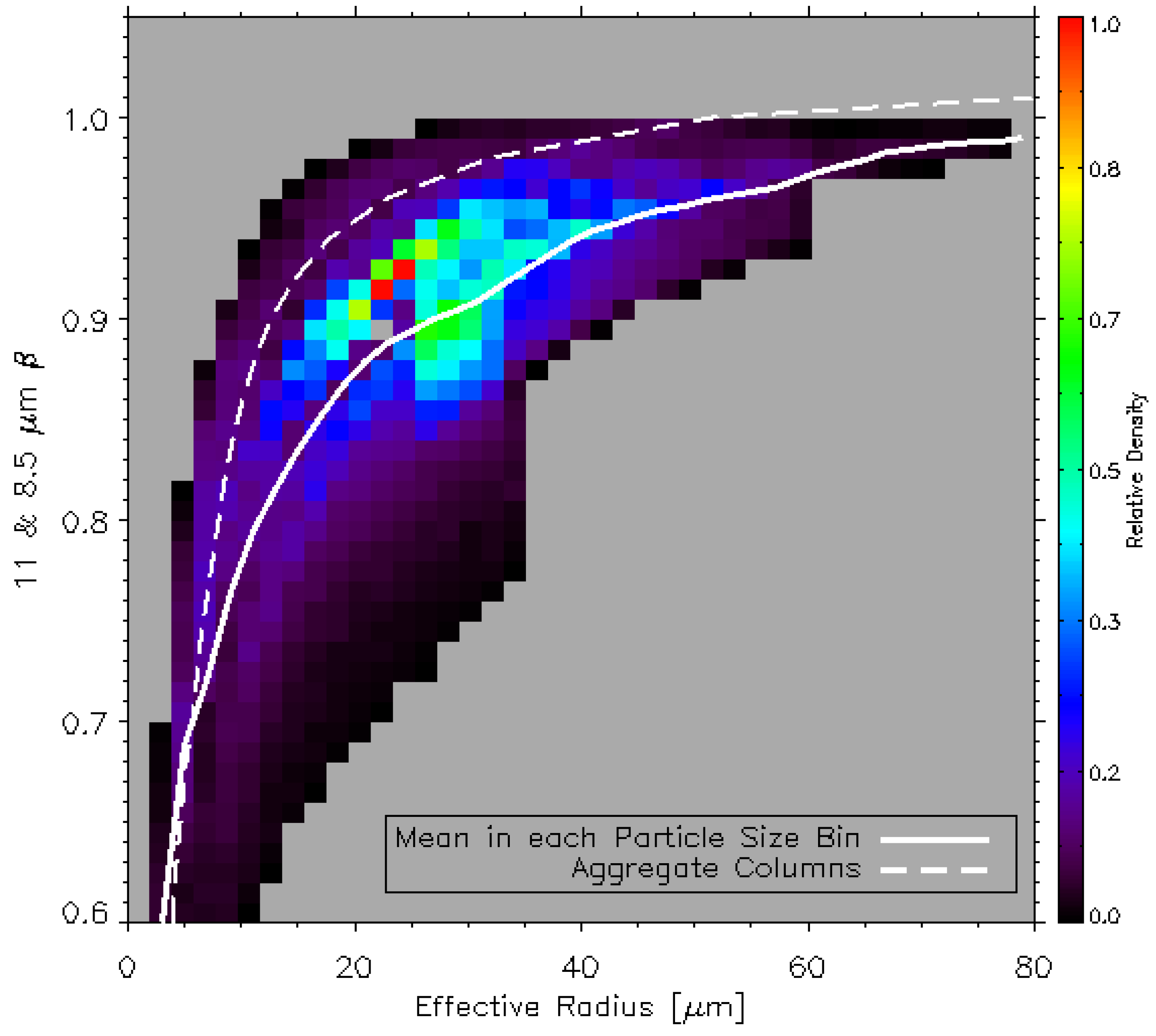
Figure 7.
Variation of the 11–8.5 μm β derived from the optimal habit solution as a function of effective radius. The training data are from a month of MODIS/CALIOP collocation in January 2010. Color values show the density of results within each β and effective radius bin. Solid white curves showing the variation of the mean β value after smoothing in each effective radius bin are used as the empirical model. Broken white curve shows the MODIS C6 aggregate column model.


 ,
, 
