
Leaf Area Index Retrieval Combining HJ1/CCD and Landsat8/OLI Data in the Heihe River Basin, China

 ,
, 
 ,
,  ,
, 
 and
and
Abstract
:
1. Introduction
2. Methodology
2.1. Analysis Method of the Multi-Sensor Dataset Characteristics
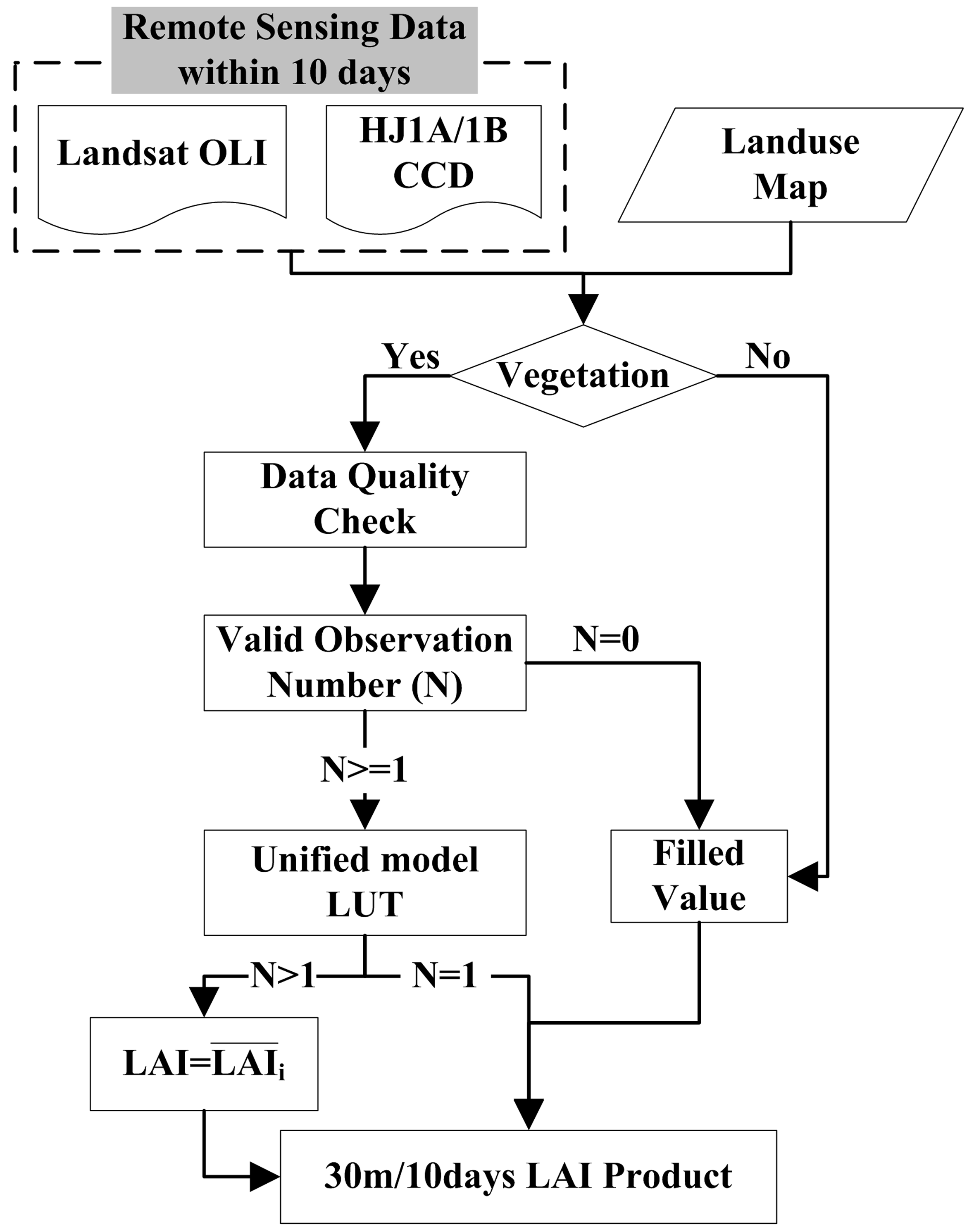
2.2. Algorithm of LAI Inversion based on the Multi-Sensor Dataset
2.2.1 Data Quality Control
- (1)
- When the NDVI difference for all of the observations in a period was greater than 0.3, the observation with the lower NDVI will be eliminated.
- (2)
- When the reflectance difference at the same or similar observation angles was greater than 15% of reflectance, the observation with the lower NDVI will be eliminated.
2.2.2. LAI Retrieval Method
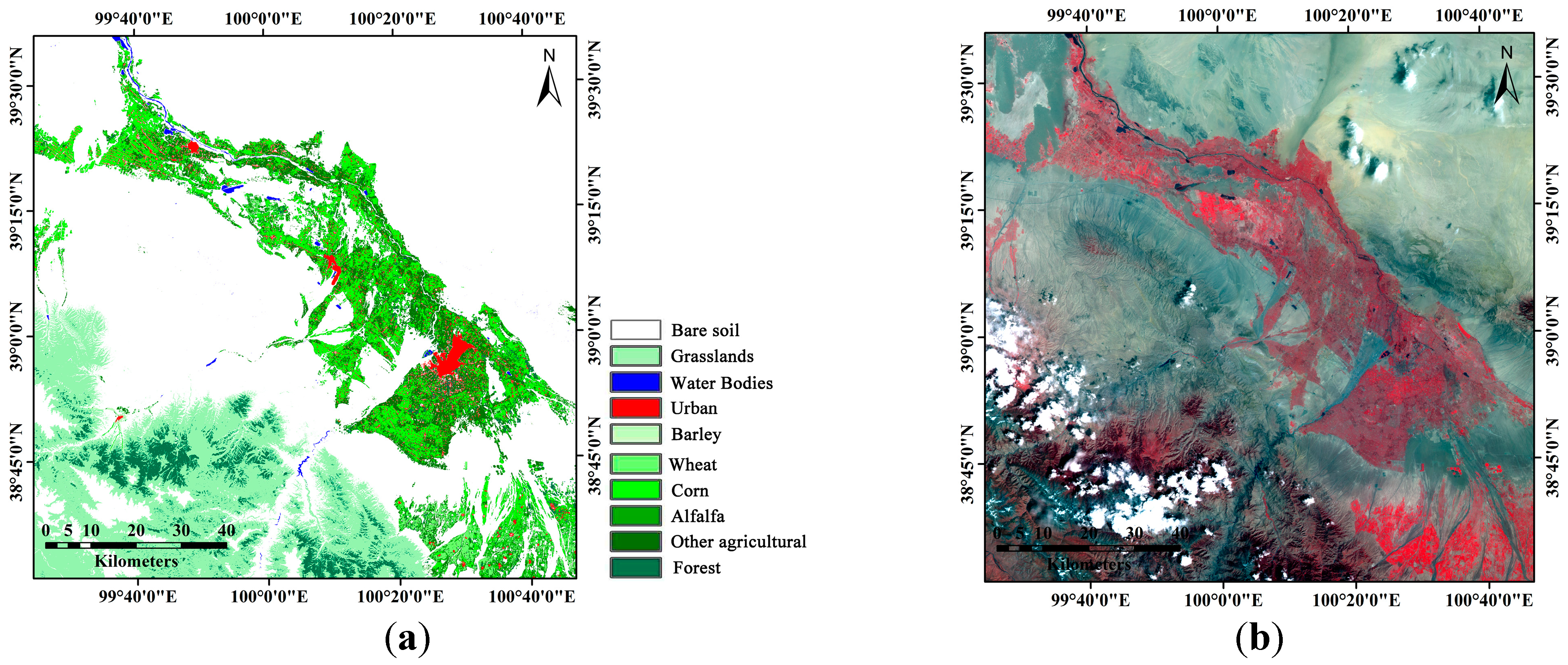
3. Study Area and Data
3.1. Study Area
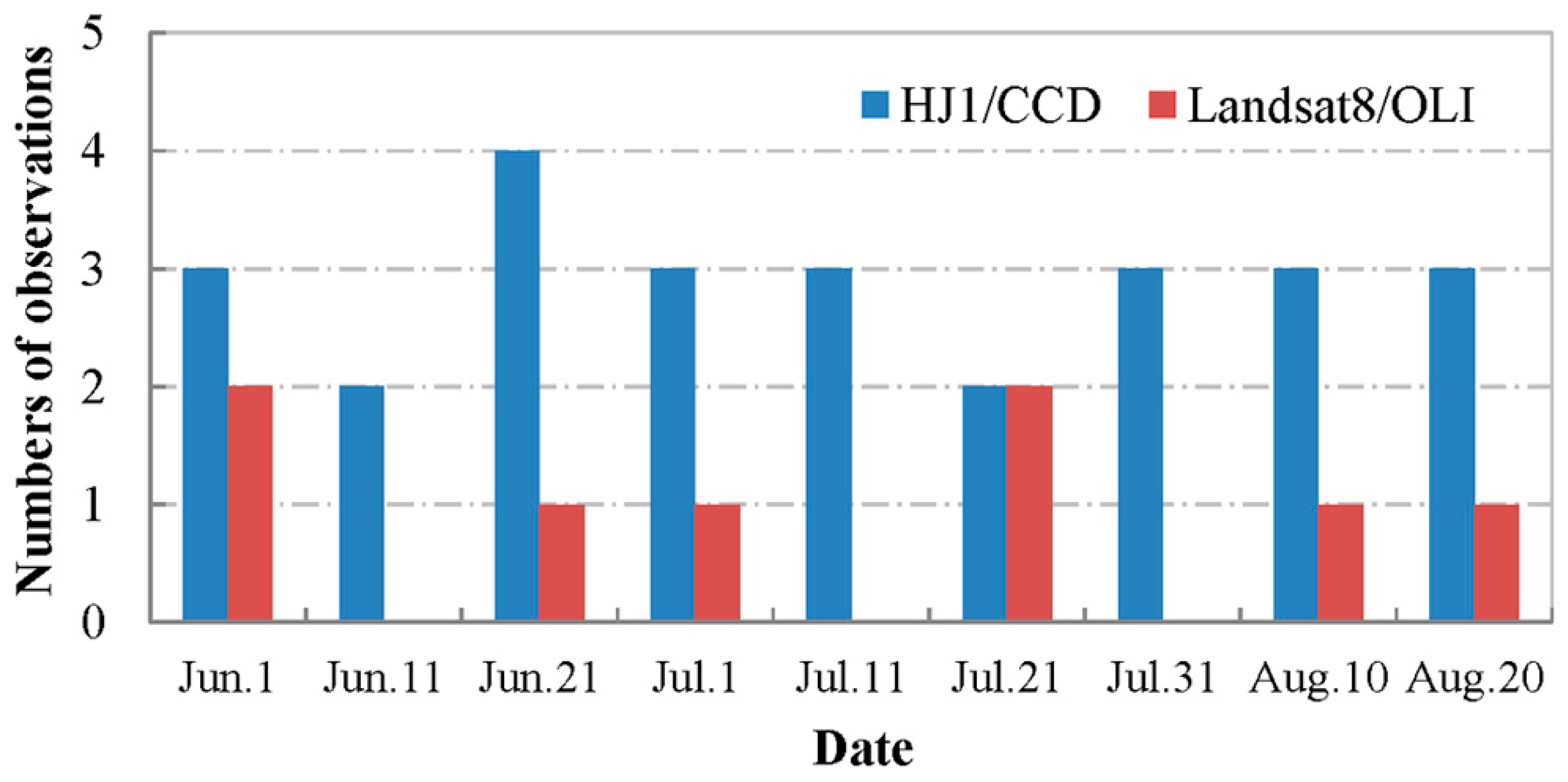
3.2. Satellite Data

| Sensor | HJ1/CCD | Landsat8/OLI | ||
|---|---|---|---|---|
| Spectral characteristics | Band | Spectral range (µm) | Band | Spectral range (µm) |
| 1 | 0.43–0.52 | 2 | 0.45–0.515 | |
| 2 | 0.52–0.60 | 3 | 0.525–0.60 | |
| 3 | 0.63–0.69 | 4 | 0.63–0.68 | |
| 4 | 0.76–0.90 | 5 | 0.845–0.885 | |
| Spatial resolution (m) | 30 | 30 | ||
| Swath width (km) | 360 (single), 700 (two) | 170 × 185 | ||
| Revisit time (days) | 4 | 16 | ||
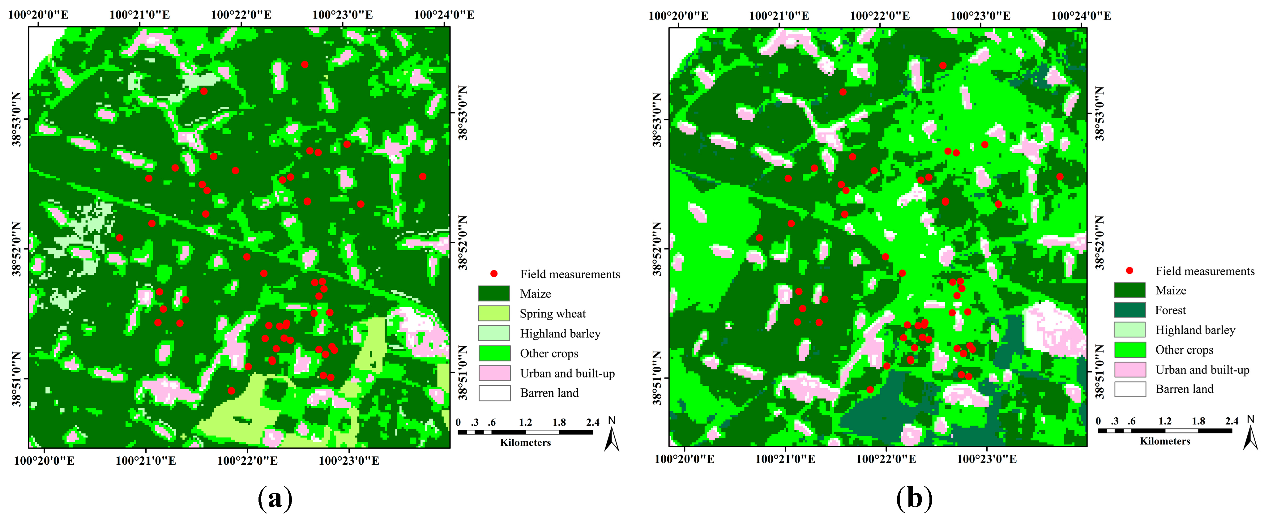
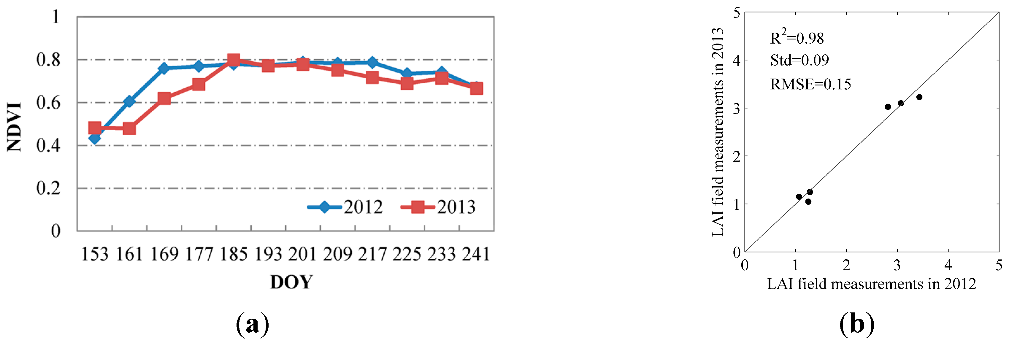
3.3. LAI Field Measurements
| Lat (°) | Lon (°) | LAI Measurements in 2012 | |||||||
|---|---|---|---|---|---|---|---|---|---|
| 11th Jun. | 21st Jun. | 1st Jul. | 11th Jul. | 21st Jul. | 31st Jul. | 10th Aug. | 20th Aug. | ||
| 100°21′11.16″E | 38°51′31.28″N | -- | 1.97 | 3.14 | 3.09 | 3.03 | 3.33 | 2.69 | 3.00 |
| 100°21′37.08″E | 38°52′14.92″N | 1.01 | 2.58 | -- | 3.82 | -- | 2.91 | 2.71 | -- |
| 100°21′55.08″E | 38°52′34.79″N | 1.14 | -- | 3.33 | 3.31 | 3.52 | 3.02 | -- | 3.14 |
| 100°21′03.96″E | 38°52′31.80″N | 1.13 | -- | -- | 3.89 | 3.73 | 3.51 | 4.07 | 3.09 |
| 100°21′37.08″E | 38°53′11.69″N | 0.94 | 2.79 | 3.76 | 3.50 | -- | 3.64 | -- | -- |
| 100°22′36.84″E | 38°53′23.32″N | 1.12 | -- | 3.44 | -- | 4.13 | 3.28 | -- | 3.02 |
| 100°23′45.60″E | 38°52′30.68″N | 1.41 | 2.21 | 3.47 | 2.87 | 3.27 | 2.99 | 2.41 | 3.20 |
| 100°22′22.44″E | 38°51′16.99″N | 0.87 | 1.93 | 3.45 | -- | 3.33 | 3.86 | 3.42 | 2.53 |
| 100°21′50.76″E | 38°50′53.09″N | 1.14 | 2.92 | -- | 3.03 | 3.38 | -- | -- | 3.23 |
| 100°22′11.28″E | 38°51′16.96″N | -- | -- | 2.82 | 3.42 | 3.83 | 3.79 | 3.45 | 2.65 |
| 100°21′24.48″E | 38°51′35.39″N | -- | 2.98 | -- | 3.06 | 3.35 | 3.05 | 3.33 | 3.30 |
| 100°22′46.56″E | 38°51′09.25″N | -- | -- | -- | 2.99 | 2.94 | 2.59 | 2.64 | 1.89 |
| Lat. | Lon. | LAI Measured on 11th–18th June 2013 | Lat. | Lon. | LAI Measured on 4th–10th July 2013 |
|---|---|---|---|---|---|
| 100°23′09.96″E | 38°52′56.99″N | 0.96 | 100°22′16.32″E | 38°51′16.34″N | 3.39 |
| 100°22′38.28″E | 38°52′11.21″N | 1.17 | 100°22′49.80″E | 38°51′28.12″N | 2.78 |
| 100°21′24.48″E | 38°52′20.32″N | 1.37 | 100°22′37.56″E | 38°51′28.40″N | 2.35 |
| 100°21′35.28″E | 38°52′27.80″N | 1.60 | 100°21′41.40″E | 38°52′41.12″N | 3.87 |
| 100°21′45.00″E | 38°52′38.10″N | 1.53 | 100°21′20.52″E | 38°52′36.16″N | 3.56 |
| 100°20′57.48″E | 38°52′54.52″N | 1.70 | 100°21′38.16″E | 38°52′25.54″N | 3.07 |
| 100°20′55.32″E | 38°52′23.59″N | 1.92 | 100°21′05.04″E | 38°52′11.21″N | 3.16 |
| 100°21′54.72″E | 38°53′06.20″N | 1.91 | 100°24′43.20″E | 38°51′16.09″N | 3.08 |
| 100°23′02.76″E | 38°52′07.40″N | 1.13 | 100°22′30.36″E | 38°45′30.64″N | 3.24 |
| 100°23′13.92″E | 38°52′37.99″N | 1.06 | 100°23′11.40″E | 38°47′40.63″N | 4.50 |
| 100°22′16.32″E | 38°52′36.98″N | 1.66 | 100°22′41.88″E | 38°47′47.62″N | 4.12 |
| 100°22′04.80″E | 38°51′30.40″N | 1.24 | 100°24′05.04″E | 38°48′50.80″N | 2.31 |
| 100°22′55.20″E | 38°51′39.89″N | 1.16 | |||
| 100°20′57.84″E | 38°51′47.81″N | 1.28 | |||
| 100°21′45.72″E | 38°51′46.01″N | 1.41 | |||
| 100°22′15.60″E | 38°51′46.40″N | 1.89 | |||
| 100°20′52.08″E | 38°20′02.05″N | 1.10 |
4. Results and Discussion
4.1. Analysis Results of the Multi-Sensor Dataset Characteristics
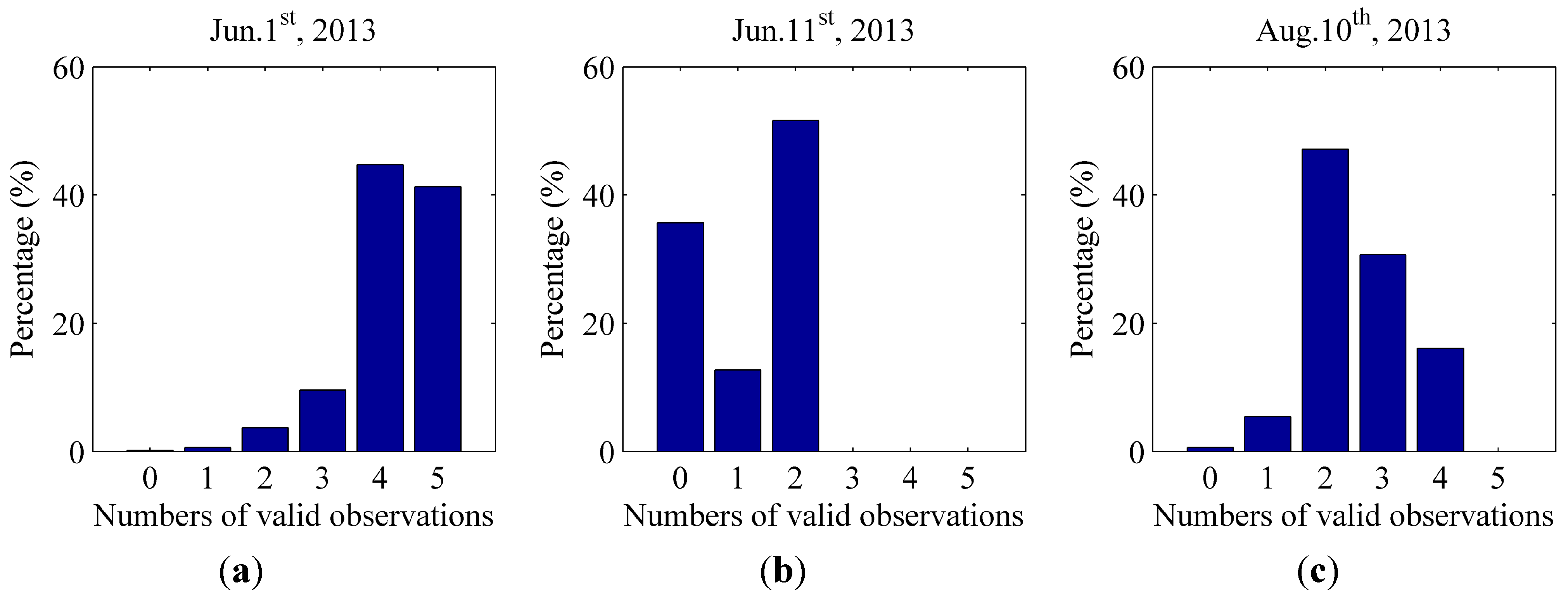
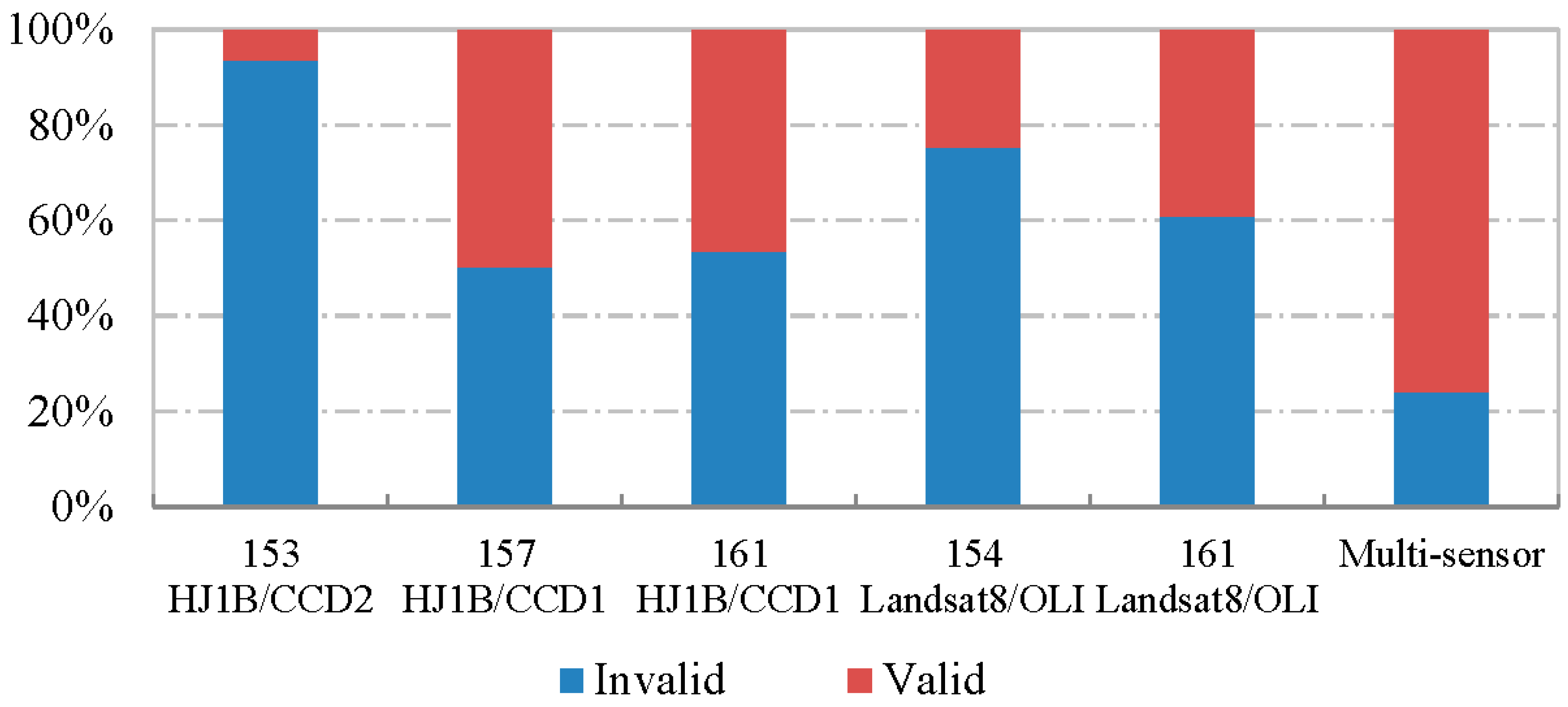
4.1.1. Percentage of Valid Observations
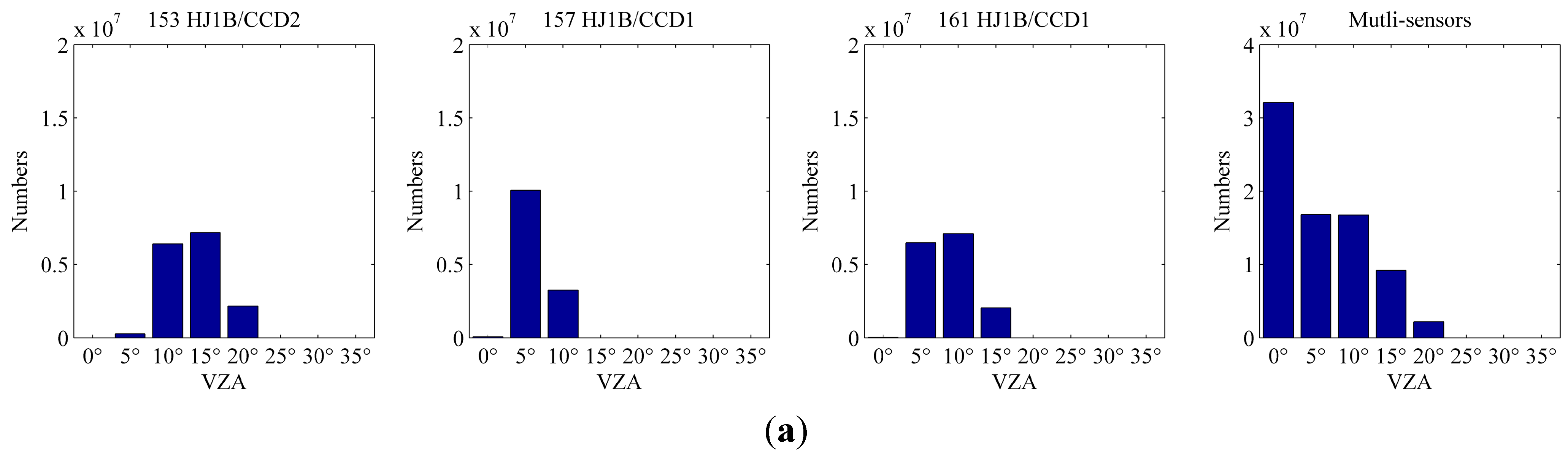
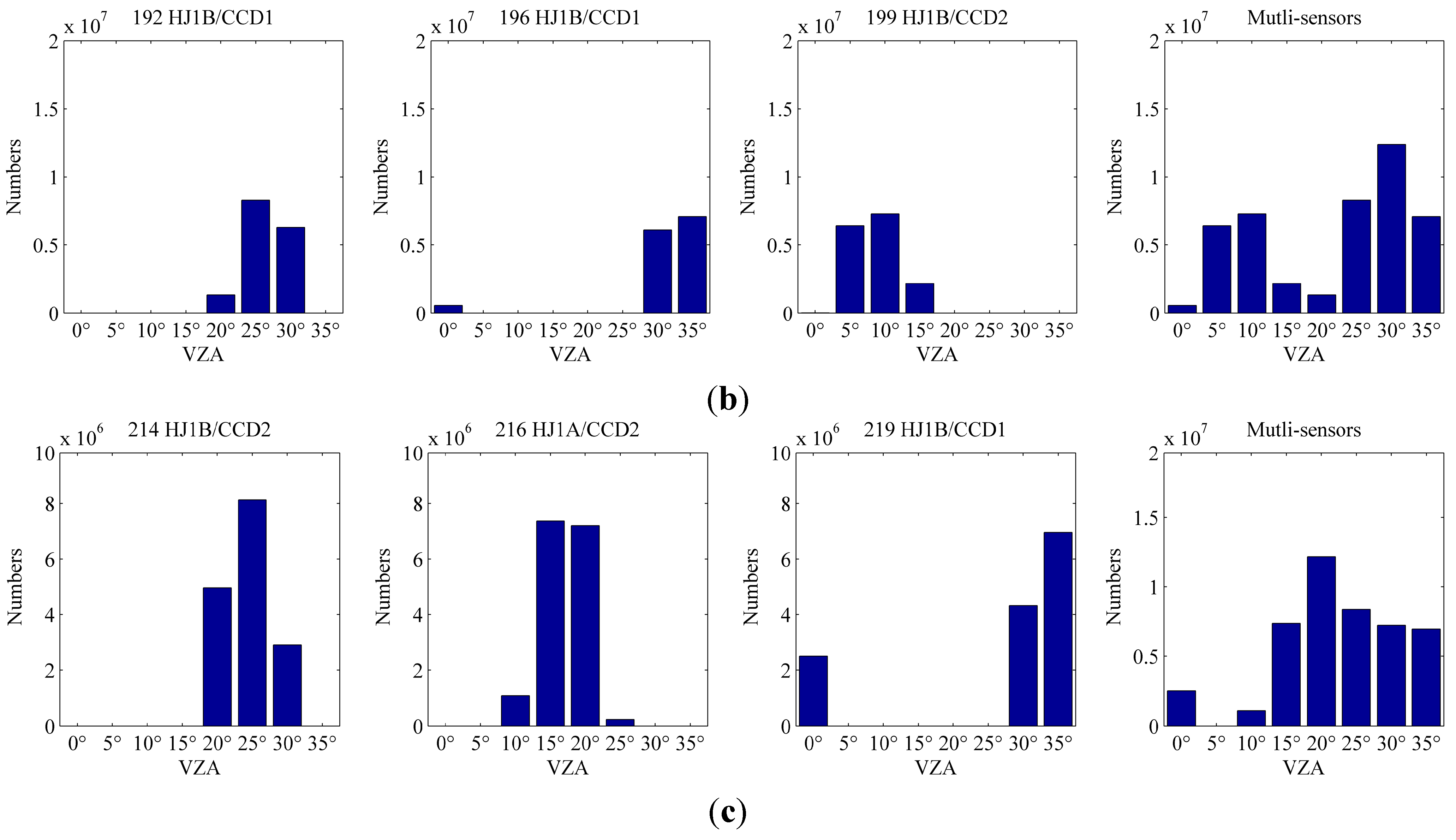
4.1.2. Distribution of Observation Angles
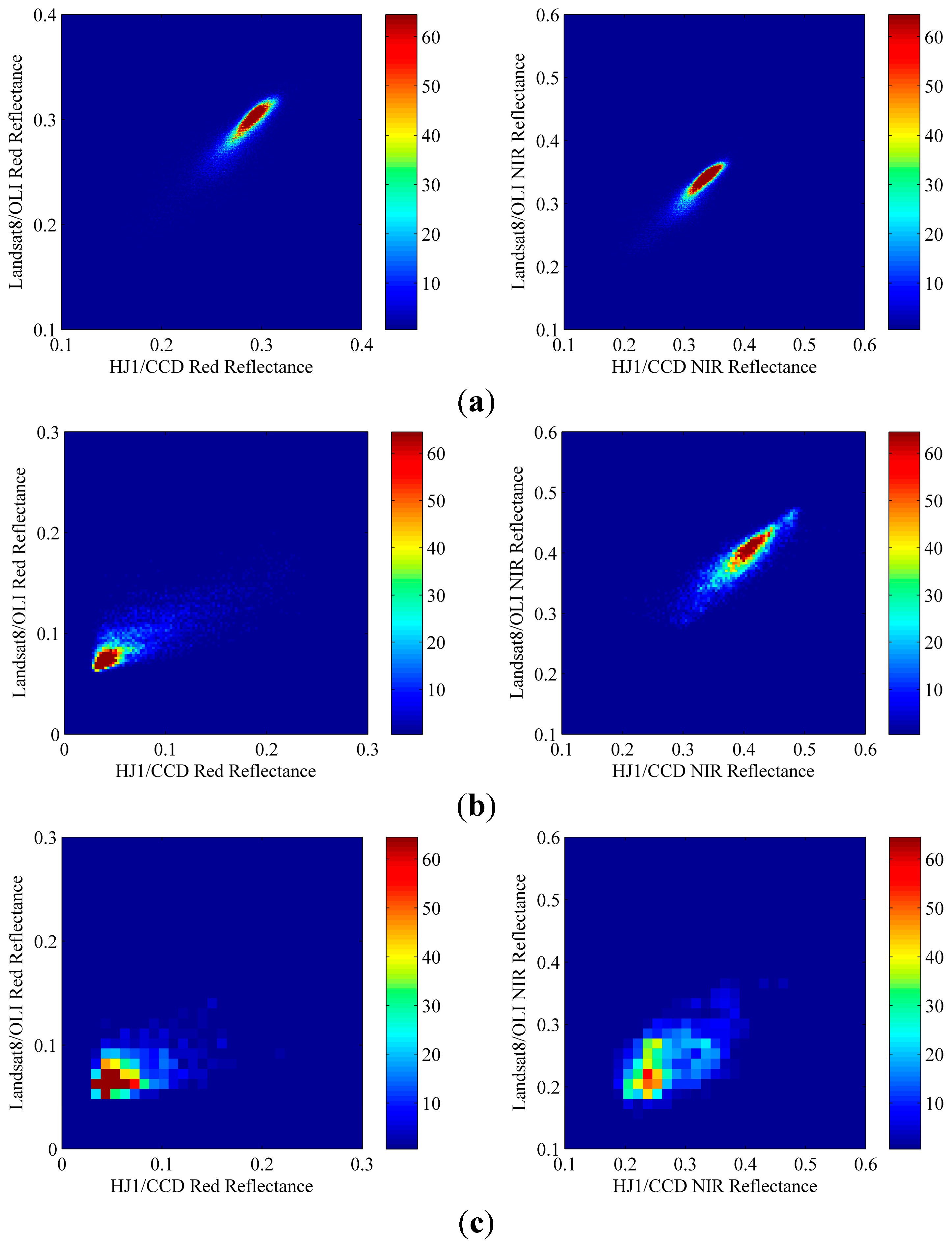
4.1.3. Variation between Different Sensor Observations
| Types | Bands | Samples | R2 | RMSE | Std. | Confidence Interval * | Homoscedasticity |
|---|---|---|---|---|---|---|---|
| Bare soil | Red | 120,700 | 0.88 | 0.01 | 0.01 | 94%–96% | No |
| NIR | 120,700 | 0.89 | 0.01 | 0.01 | 88%–91% | No | |
| Crop | Red | 14,550 | 0.79 | 0.04 | 0.02 | 33%–35% | No |
| NIR | 14,534 | 0.86 | 0.02 | 0.02 | 66%–70% | No | |
| Forest | Red | 1529 | 0.50 | 0.03 | 0.02 | 26%–32% | No |
| NIR | 1518 | 0.59 | 0.06 | 0.03 | 55%–67% | No |

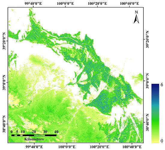
4.2. LAI Inversion Results and Validation

4.2.1. Improvement of the Valid LAI Inversion from the Multi-Sensor Dataset
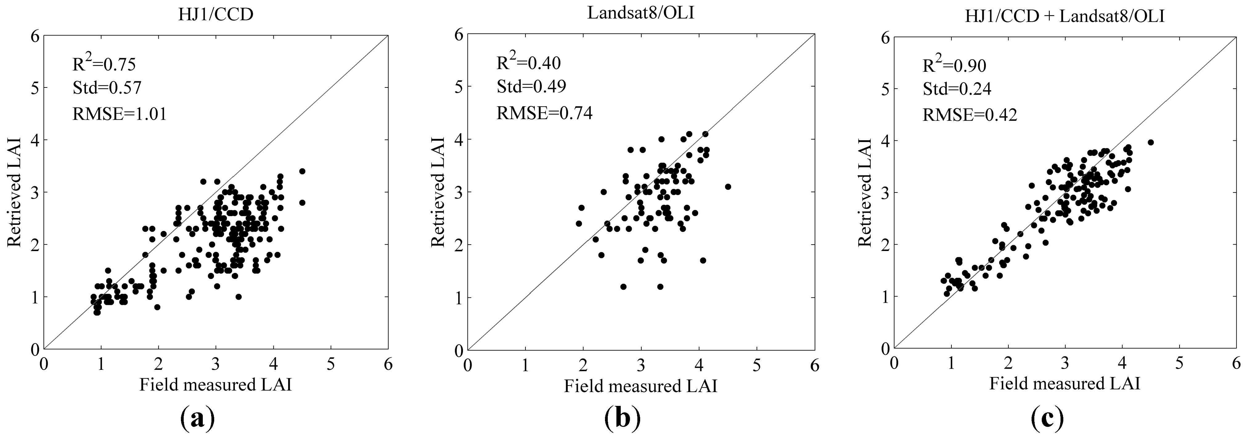
4.2.2. Validation

4.2.3. Comparison of LAI Inversions with Existing Studies
5. Conclusions
Acknowledgments
Author Contributions
Conflicts of Interest
References
- Chen, J.M.; Black, T.A. Measuring leaf area index of plant canopies with branch architecture. Agric. For. Meteorol. 1991, 57, 1–12. [Google Scholar] [CrossRef]
- Chen, J.M.; Black, T.A. Defining leaf area index for non-flat leaves. Plant Cell Environ. 1992, 15, 421–429. [Google Scholar] [CrossRef]
- Fang, H.; Liang, S.; Kuusk, A. Retrieving leaf area index using a genetic algorithm with a canopy radiative transfer model. Remote Sens. Environ. 2003, 85, 257–270. [Google Scholar] [CrossRef]
- Chen, J.M.; Pavlic, G.; Brown, L.; Cihlar, J.; Leblanc, S.; White, H.; Hall, R.; Peddle, D.; King, D.; Trofymow, J. Derivation and validation of Canada-wide coarse-resolution leaf area index maps using high-resolution satellite imagery and ground measurements. Remote Sens. Environ. 2002, 80, 165–184. [Google Scholar] [CrossRef]
- Wan, H.; Wang, J.; Xiao, Z.; Li, L. Generating the high spatial and temporal resolution LAI by fusing MODIS and ASTER. J. Beijing Norm. Univ. (Nat. Sci.) 2007, 43, 303–308. (In Chinese) [Google Scholar]
- Weiss, M.; Baret, F. Evaluation of canopy biophysical variable retrieval performances from the accumulation of large swath satellite data. Remote Sens. Environ. 1999, 70, 293–306. [Google Scholar] [CrossRef]
- Fassnacht, K.S.; Gower, S.T.; MacKenzie, M.D.; Nordheim, E.V.; Lillesand, T.M. Estimating the leaf area index of north central Wisconsin forests using the Landsat Thematic Mapper. Remote Sens. Environ. 1997, 61, 229–245. [Google Scholar] [CrossRef]
- Fernandes, R.; Butson, C.; Leblanc, S.; Latifovic, R. Landsat-5 TM and Landsat-7 ETM+ based accuracy assessment of leaf area index products for Canada derived from SPOT-4 VEGETATION data. Can. J. Remote Sens. 2003, 29, 241–258. [Google Scholar] [CrossRef]
- Tian, Q.J.; Jin, Z.Y. Research on calculation and spatial scaling of forest leaf area index from remote sensing image. Remote Sens. Inf. 2006, 5–11. [Google Scholar]
- Zhu, G.L.; Ju, W.M.; Chen, J.M.; Fan, W.Y.; Zhou, Y.L.; Li, X.F.; Li, M.Z. Forest canopy leaf area index in Maoershan Mountain: Groundmeasurement and remote sensing retrieval. Chin. J. Appl. Ecol. 2010, 21, 2117–2124. [Google Scholar]
- Deng, F.; Chen, J.M.; Plummer, S.; Chen, M.; Pisek, J. Algorithm for global leaf area index retrieval using satellite imagery. IEEE Trans. Geosci. Remote Sens. 2006, 44, 2219–2229. [Google Scholar] [CrossRef]
- Masson, V.; Champeaux, J.-L.; Chauvin, F.; Meriguet, C.; Lacaze, R. A global database of land surface parameters at 1-km resolution in meteorological and climate models. J. Clim. 2003, 16, 1261–1282. [Google Scholar] [CrossRef]
- Knyazikhin, Y.; Glassy, J.; Privette, J.; Tian, Y.; Lotsch, A.; Zhang, Y.; Wang, Y.; Morisette, J.; Votava, P.; Myneni, R. Modis Leaf Area Index (LAI) and Fraction of Photosynthetically Active Radiation Absorbed by Vegetation (FPAR) Product (Mod15) Algorithm Theoretical Basis Document; Theoretical Basis Document; NASA Goddard Space Flight Center: Greenbelt, MA, USA, 1999.
- Baret, F.; Hagolle, O.; Geiger, B.; Bicheron, P.; Miras, B.; Huc, M.; Berthelot, B.; Niño, F.; Weiss, M.; Samain, O. LAI, fAPAR and fCover CYCLOPES global products derived from VEGETATION: Part 1: Principles of the algorithm. Remote Sens. Environ. 2007, 110, 275–286. [Google Scholar] [CrossRef] [Green Version]
- Ganguly, S.; Schull, M.A.; Samanta, A.; Shabanov, N.V.; Milesi, C.; Nemani, R.R.; Knyazikhin, Y.; Myneni, R.B. Generating vegetation leaf area index earth system data record from multiple sensors. Part 1: Theory. Remote Sens. Environ. 2008, 112, 4333–4343. [Google Scholar] [CrossRef]
- Knyazikhin, Y.; Martonchik, J.; Myneni, R.; Diner, D.; Running, S. Synergistic algorithm for estimating vegetation canopy leaf area index and fraction of absorbed photosynthetically active radiation from MODIS and MISR data. J. Geophys. Res. Atmos. 1998, 103, 32257–32275. [Google Scholar] [CrossRef]
- Gascon, F.; Gastellu-Etchegorry, J.P.; Leroy, M. Using multi-directional high-resolution imagery from POLDER sensor to retrieve leaf area index. Int. J. Remote Sens. 2007, 28, 167–181. [Google Scholar] [CrossRef] [Green Version]
- Baret, F.; Weiss, M.; Lacaze, R.; Camacho, F.; Makhmara, H.; Pacholcyzk, P.; Smets, B. GEOV1: LAI and FAPAR essential climate variables and FCOVER global time series capitalizing over existing products. Part 1: Principles of development and production. Remote Sens. Environ. 2013, 137, 299–309. [Google Scholar] [CrossRef]
- Liang, S.; Zhao, X.; Liu, S.; Yuan, W.; Cheng, X.; Xiao, Z.; Zhang, X.; Liu, Q.; Cheng, J.; Tang, H. A long-term Global LAnd Surface Satellite (GLASS) data-set for environmental studies. Int. J. Digit. Earth. 2013, 6, 5–33. [Google Scholar] [CrossRef]
- Xiao, Z.; Liang, S.; Wang, J.; Chen, P.; Yin, X.; Zhang, L.; Song, J. Use of general regression neural networks for generating the GLASS leaf area index product from time-series MODIS surface reflectance. IEEE Trans. Geosci. Remote Sens. 2014, 52, 209–223. [Google Scholar] [CrossRef]
- Mousivand, A.; Menenti, M.; Gorte, B.; Verhoef, W. Multi-temporal, multi-sensor retrieval of terrestrial vegetation properties from spectral–directional radiometric data. Remote Sens. Environ. 2015, 158, 311–330. [Google Scholar] [CrossRef]
- Wan, H.W. Surface Parameters Inversion from Multi-Source Remote Sensing Data Fusion Study. Ph.D Thesis, Beijing Normal University, Beijing, China, 2007. [Google Scholar]
- Liang, S.; Zhang, X.; Xiao, Z.; Cheng, J.; Liu, Q.; Zhao, X. Global Surface Energy Budget and Ecosystem Variables (Glass) Product Algorithm, Validation and Analysis; Higher Education Press: Beijing, China, 2014. (In Chinese) [Google Scholar]
- Ganguly, S.; Nemani, R.R.; Zhang, G.; Hashimoto, H.; Milesi, C.; Michaelis, A.; Wang, W.; Votava, P.; Samanta, A.; Melton, F. Generating global leaf area index from landsat: Algorithm formulation and demonstration. Remote Sens. Environ. 2012, 122, 185–202. [Google Scholar] [CrossRef]
- Wan, H.W.; Wang, J.; Liang, S.; Qin, J. Combine MODIS and MISR data to retrieval LAI. Spectrosc. Spectr. Anal. 2009, 29, 3106–3111. [Google Scholar]
- Hagolle, O.; Lobo, A.; Maisongrande, P.; Cabot, F.; Duchemin, B.; De Pereyra, A. Quality assessment and improvement of temporally composited products of remotely sensed imagery by combination of VEGETATION 1 and 2 images. Remote Sens. Environ. 2004, 94, 172–186. [Google Scholar] [CrossRef] [Green Version]
- Morton, D.C.; Nagol, J.; Carabajal, C.C.; Rosette, J.; Palace, M.; Cook, B.D.; Vermote, E.F.; Harding, D.J.; North, P.R. Amazon forests maintain consistent canopy structure and greenness during the dry season. Nature 2014, 506, 221–224. [Google Scholar] [CrossRef] [PubMed]
- Ju, J.; Roy, D.P.; Shuai, Y.; Schaaf, C. Development of an approach for generation of temporally complete daily nadir MODIS reflectance time series. Remote Sens. Environ. 2010, 114, 1–20. [Google Scholar] [CrossRef]
- Zhang, Y.H. HJ1-CCD Cross Radiometric Calibration. Master Themes, Shandong University of Science and Technology, Qingdao, China, 2011. [Google Scholar]
- Leblanc, S.G.; Chen, J.M.; Cihlar, J. NDVI directionality in boreal forests: A model interpretation of measurements. Can. J. Remote Sens. 1997, 23, 369–380. [Google Scholar] [CrossRef]
- Walter, E.; Privette, J.; Cornell, D.; Mesarch, M.A.; Hays, C. Relations between directional spectral vegetation indices and leaf area and absorbed radiation in alfalfa. Remote Sens. Environ. 1997, 61, 162–177. [Google Scholar] [CrossRef]
- Chen, J.; Menges, C.; Leblanc, S. Global mapping of foliage clumping index using multi-angular satellite data. Remote Sens. Environ. 2005, 97, 447–457. [Google Scholar] [CrossRef]
- Yan, B.; Xu, X.; Fan, W. A unified canopy bidirectional reflectance (BRDF) model for row ceops. Sci. China Press. 2012, 42, 411–423. [Google Scholar] [CrossRef]
- Fan, W.; Xu, X.; Liu, X.; Yan, B.; Cui, Y. Accurate LAI retrieval method based on PROBA/CHRIS data. Hydrol. Earth Syst. Sci. 2010, 14, 1499–1507. [Google Scholar] [CrossRef]
- Fan, W.; Yan, B.; Xu, X. Crop area and leaf area index simultaneous retrieval based on spatial scaling transformation. Sci. China Earth Sci. 2010, 53, 1709–1716. [Google Scholar] [CrossRef]
- Li, X.; Li, X.W.; Li, Z.Y.; Ma, M.G.; Wang, J.; Xiao, Q.; Liu, Q.; Che, T.; Chen, E.X.; Yan, G.J.; et al. Watershed allied telemetry experimental research. J. Geophys. Res. 2009, 114. [Google Scholar] [CrossRef]
- Li, X.; Cheng, G.D.; Liu, S.M.; Xiao, Q.; Ma, M.G.; Jin, R.; Che, T.; Liu, Q.H.; Wang, W.Z.; Qi, Y.; et al. Heihe Watershed Allied Telemetry Experimental Research (HiWATER): Scientific objectives and experimental design. Bull. Am. Meteorol. Soc. 2013, 94, 1145–1160. [Google Scholar] [CrossRef]
- Cheng, G.D.; Li, X.; Zhao, W.Z.; Xu, Z.M.; Feng, Q.; Xiao, S.C.; Xiao, H.L. Integrated study of the water-ecosystem-economy in the Heihe River Basin. Natl. Sci. Rev. 2014, 1, 413–428. [Google Scholar] [CrossRef]
- USGS. Earthexplorer. Available online: http://earthexplorer.usgs.gov/ (accessed on 18 February 2015).
- China Centre for Resources Satellite Data and Application. Available online: http://www.cresda.com/n16/index.html (accessed on 18 February 2015).
- Zhong, B.; Li, H.; Shan, X.; Mu, X.; Wu, H.; Chen, X.; Liu, Y. Architecture of Multisource Data Processing System (ADPS); No. 2012AA12A304; Institute of Remote Sensing and Digital Earth, Chinese Academy of Sciences: Beijing, China, 2014. [Google Scholar]
- Zhong, B.; Zhang, Y.; Du, T.; Yang, A.; Lv, W.; Liu, Q. Cross-calibration of HJ-1/CCD over a desert site using Landsat ETM imagery and ASTER GDEM product. IEEE Trans. Geosci. Remote Sens. 2014, 52, 7247–7263. [Google Scholar] [CrossRef]
- Shan, X.J.; Tang, P.; Hu, C.M.; Tang, L.; Zheng, K. Automatic geometric precise correction technology and system based on hierarchical image matching for HJ-1A/B CCD images. J. Remote Sens. 2014, 2, 254–266. [Google Scholar]
- Zhong, B. Improved estimation of aerosol optical depth from Landsat TM/ETM+ imagery over land. In Proceedings of 2011 IEEE International Geoscience and Remote Sensing Symposium (IGARSS), Vancouver, BC, Canada, 24–29 July 2011; pp. 3304–3307.
- Zhong, B.; Wu, S.; Yang, A.; Liu, Q. An improved aerosol optical depth retrieval algorithm for moderate to high spatial resolution optical remotely sensed imagery. IEEE Trans. Geosci. Remote Sens. 2015. (Under Review). [Google Scholar]
- Zeng, Y.; Li, J.; Liu, Q.; Qu, Y.; Huete, A.R.; Xu, B.; Yin, G.; Zhao, J. An optimal sampling design for observing and validating long-term leaf area index with temporal variations in spatial heterogeneities. Remote Sens. 2015, 7, 1300–1319. [Google Scholar] [CrossRef]
- Chen, B.; Coops, N.C.; Fu, D.; Margolis, H.A.; Amiro, B.D.; Black, T.A.; Arain, M.A.; Barr, A.G.; Bourque, C.P.A.; Flanagan, L.B.; et al. Characterizing spatial representativeness of flux tower eddy-covariance measurements across the Canadian Carbon Program Network using remote sensing and footprint analysis. Remote Sens. Environ. 2012, 124, 742–755. [Google Scholar] [CrossRef]
- Qu, Y.; Wang, J.; Dong, J.; Jiang, F. Design and experiment of crop structural parameters automatic measurement system. Trans. Chin. Soc. Agric. Eng. 2012, 28, 160–165. [Google Scholar]
© 2015 by the authors; licensee MDPI, Basel, Switzerland. This article is an open access article distributed under the terms and conditions of the Creative Commons Attribution license (http://creativecommons.org/licenses/by/4.0/).
Share and Cite
Zhao, J.; Li, J.; Liu, Q.; Fan, W.; Zhong, B.; Wu, S.; Yang, L.; Zeng, Y.; Xu, B.; Yin, G. Leaf Area Index Retrieval Combining HJ1/CCD and Landsat8/OLI Data in the Heihe River Basin, China. Remote Sens. 2015, 7, 6862-6885. https://doi.org/10.3390/rs70606862
Zhao J, Li J, Liu Q, Fan W, Zhong B, Wu S, Yang L, Zeng Y, Xu B, Yin G. Leaf Area Index Retrieval Combining HJ1/CCD and Landsat8/OLI Data in the Heihe River Basin, China. Remote Sensing. 2015; 7(6):6862-6885. https://doi.org/10.3390/rs70606862
Chicago/Turabian StyleZhao, Jing, Jing Li, Qinhuo Liu, Wenjie Fan, Bo Zhong, Shanlong Wu, Le Yang, Yelu Zeng, Baodong Xu, and Gaofei Yin. 2015. "Leaf Area Index Retrieval Combining HJ1/CCD and Landsat8/OLI Data in the Heihe River Basin, China" Remote Sensing 7, no. 6: 6862-6885. https://doi.org/10.3390/rs70606862