Tracking Land Use/Land Cover Dynamics in Cloud Prone Areas Using Moderate Resolution Satellite Data: A Case Study in Central Africa

Abstract

Tracking land surface dynamics over cloud prone areas with complex mountainous terrain is an important challenge facing the Earth Science community. One such region is the Lake Kivu region in Central Africa. We developed a processing chain to systematically monitor the spatio-temporal land use/land cover dynamics of this region over the years 1988, 2001, and 2011 using Landsat data, complemented by ancillary data. Topographic compensation was performed on Landsat reflectances to avoid the strong illumination angle impacts and image compositing was used to compensate for frequent cloud cover and thus incomplete annual data availability in the archive. A systematic supervised classification was applied to the composite Landsat imagery to obtain land cover thematic maps with overall accuracies of 90% and higher. Subsequent change analysis between these years found extensive conversions of the natural environment as a result of human related activities. The gross forest cover loss for 1988–2001 and 2001–2011 period was 216.4 and 130.5 thousand hectares, respectively, signifying significant deforestation in the period of civil war and a relatively stable and lower deforestation rate later, possibly due to conservation and reforestation efforts in the region. The other dominant land cover changes in the region were aggressive subsistence farming and urban expansion displacing natural vegetation and arable lands. Despite limited data availability, this study fills the gap of much needed detailed and updated land cover change information for this biologically important region of Central Africa. These multi-temporal datasets will be a valuable baseline for land use managers in the region interested in developing ecologically sustainable land management strategies and measuring the impacts of biodiversity conservation efforts.

1. Introduction

Human-induced land cover change is increasingly affecting the biophysics, biogeochemistry and biogeography of the Earth’s surface and the atmosphere [1]. These changes are occurring at a range of spatial scales from local to global and at temporal frequencies of days to millennia [2]. Land-cover changes play a significant role in the global carbon cycle, both as a source and a sink [3]. The need for understanding the distribution and dynamics of land cover can never be underestimated due to its huge implications to human well-being. Hansen and Loveland (2012) [4] emphasizes the need for timely, accurate observations documenting land cover change to be more pressing than ever given the changing state of global climate. Accurate and up-to-date information on land cover and land cover change is therefore required for applications like managing natural resources and monitoring environmental changes. However, there have been relatively few efforts to identify the spatial and temporal patterns of land cover change in the Lake Kivu region, the focus of this study.

Situated at the high point of the western branch of the East African Rift valley, the Lake Kivu region is densely populated with intensive agriculture on steep slopes, yet remains a biodiversity hotspot consisting of remnant and protected montane forests with endemic wildlife, birds and fish species [5,6]. Land cover mapping of the Lake Kivu region has previously been carried out by United Nations Food and Agriculture Organization (FAO) in its Africover project by producing single time frame multipurpose land cover maps of DRC, Rwanda, Burundi, and Uganda using Landsat imagery acquired around 1999–2001 [7]. On the other hand, the priority of a number of researchers has been forest cover change in the Congo Basin. For example, Potapov et al. (2012) [8] quantified forest cover loss in the DRC region of the study area from 2001 to 2010 using Landsat imagery. However, that important work is solely focused on forest change. No detailed land cover change analysis of the Lake Kivu region has been accomplished.

Remote sensing satellite imagery provides an efficient and cost effective means of obtaining information on temporal trends and spatial distribution of land cover [9]. Remote sensing has been used successfully in mapping a range of land covers at a variety of spatial and temporal scales [10]. Satellite-based monitoring has one additional advantage; independence from official national agencies allowing open publication of monitoring results [8]. Landsat data constitutes the longest record of global-scale medium spatial resolution earth observation data available freely in the web since 2008 [4,11]. Landsat provides substantial insight into how the Earth has changed as far as back as 1972 when Landsat 1 was launched [12]. Due to its finer spatial resolution than many other global satellite imagers, Landsat imagery has been the data source of choice for many land cover and land use change studies [13,14,15,16,17,18]. Landsat has been widely used to study the dynamics of various earth surfaces like forest cover [19,20], grassland [21], delta [22], takir [23], urban areas [24,25], pampas [26], rangelands [27], and arid regions [18].

Landsat data are used to monitor the complex landscape in Lake Kivu region in this study. However, data gaps and a very complex landscape make this region a very challenging site to perform land cover analysis. Persistent cloud is one major limiting factor for land surface observation in humid tropical regions [28,29] like the Lake Kivu region. The region also suffers from low Landsat acquisition frequency for the early Landsat sensors because of lack of ground station coverage in central Africa and limited onboard image storage capacity, reducing temporal coverage for the application of land change methods [30,31,32]. Furthermore, the Landsat ETM+ SLC-off acquisitions suffer from wedge shape gaps reducing 22% of the usable data after 2003 [28,33,34].

The objectives of this study are to provide a recent perspective for land use/land cover types found in the dynamic and complex Lake Kivu region, to monitor the spatio-temporal dynamics of land cover change in the region over three periods (1988, 2001 and 2011), and analyze the driving forces behind the dynamics of these changes in the region.

2. Study Area

The Lake Kivu region is located in central Africa on the border between Democratic Republic of Congo, Uganda, Burundi and Rwanda. It is defined by two adjacent Landsat Worldwide Reference System (WRS-2) path/rows (173/61 and 173/62) as shown (Figure 1) and extends over 64,238 km². The region has highly diverse topography, measuring 900 m above sea level at the plains in the Rift Valley to the north to the highest peak of 4507 m at Mount Karisimbi, the largest of the eight volcanoes situated in the Virunga Mountains [35]. A typical example of the complex rural landscape in western Rwanda is shown in Figure 2. These highlands east of Lake Kivu are dominated by plateau between 1400 m and 2200 m altitude with many hills and depressions [36]. This equatorial study region, due to its high elevation, is characterized by a temperate sub-equatorial climate as the mean temperature ranges from 15 °C to 25 °C depending upon the altitude [37]. Rainfall is bimodal in distribution and occurs primarily during September–November and March–May [38]. Between these rainfalls are two dry periods, a short one between December and February and a long one from June to August [39]. The long dry season overlaps with planting season of rice, maize and beans, while the end of shorter dry season overlaps with beginning of second planting season. The average rainfall in the highland areas is greater than 2000 mm, whereas in the lowlands it reaches below 1000 mm.

One of the reasons this area has such dynamics in land use and land cover change is social upheaval due to a massive refugee crisis, civil war [40] and genocide [41] during the nineties [42]. The long-term conflict severely stressed the natural environment and subsistence agricultural system, with ongoing pressure on the highland forests for fuel use and clearing for farming [36]. Recent political stabilization has enabled a renewed focus on conservation and environmental recovery. Other land use and land cover change dynamics arise from natural forces. This region is vulnerable to natural disasters emanating from climatic and seismic disturbances causing economic damage and loss of lives, problems that are often exacerbated by the intensive land use. The major climatic disasters include drought, floods and landslides, while major seismic disturbances include earthquakes and volcanic eruptions [39,43]. In many settled areas the population density is exceptionally high (150–800 people/km²) due to its favorable climate to cultivation [44]. Currently, nearly 90 percent of the population in the region is dependent on subsistence farming for their livelihood [45,46]. However, intensive agriculture practices in the areas have led to extensive problems of soil runoff and erosion [38].

Figure 1. Location of the study area covered by two Landsat scenes: south and north (the red rectangle).

Figure 1. Location of the study area covered by two Landsat scenes: south and north (the red rectangle).

Figure 2. South facing image of a rural landscape showing steep-sided hills and small fragmented agricultural plots at approximately lat., −2.53, lon., 29.67.

Figure 2. South facing image of a rural landscape showing steep-sided hills and small fragmented agricultural plots at approximately lat., −2.53, lon., 29.67.

3. Data

3.1. Landsat Reflectance Data

This study employed the available Landsat TM/ETM+ data of the Lake Kivu region from the Landsat archive. The growing season is generally more useful for mapping vegetation than dormant periods [47]. The primary planting season in the region is during the March–May wet season. Thus the primary Landsat data were those obtained in June–August as the crops matured. When scenes were not available during the primary growing period, data with minimal cloud cover were obtained from the second dry season. The available Landsat scenes in the United State Geological Survey (USGS) archive for our region of interest were processed using the Landsat Ecosystem Disturbance Adaptive Processing System (LEDAPS) located at the USGS Earth Resources Observation and Science (EROS) Center. USGS recently implemented LEDAPS to produce the Landsat Surface Reflectance Climate Data Record (CDR) product, which was downloaded from USGS (http://earthexplorer.usgs.gov/). LEDAPS software was originally developed by the National Aeronautics and Space Administration–Goddard Space Flight Center and the University of Maryland [48]. LEDAPS produces top-of-atmosphere (TOA) reflectance from Landsat Thematic Mapper (TM) and Enhanced Thematic Mapper Plus (ETM+) Level 1 digital numbers (DN) and applies atmospheric compensation to generate a surface-reflectance product [49]. The atmospheric compensations are based on the second simulation of a satellite signal in the solar spectrum (6S) radiative transfer code [50] used by the Moderate Resolution Imaging Spectroradiometer (MODIS) Land Science Team. Detailed discussion and comparison of LEDAPS products with other processing streams are given by Ju et al. (2012) [51]. The Landsat surface reflectance CDR was delivered from EROS in Hierarchical Data Format for Earth Observing Systems (HDF-EOS) in the Universal Transverse Mercator (UTM) map projection with a World Geodetic System (WGS) 84 datum. In this paper, all analyses were performed on the six non-thermal bands of TM/ETM+, which consists of three visible and three infrared bands with spatial resolution of 30 m.

3.2. Digital Elevation Model

At the time of this study, the LEDAPS processing of Landsat imagery does not include terrain correction [49]. Thus a topographic correction was needed to compensate for the very significant terrain illumination effects for the study region. The Digital Elevation Model (DEM) used in this study is the Advanced Spaceborne Thermal Emission and Reflection Radiometer (ASTER) Global Digital Elevation Model (GDEM) version 2. The ASTER DEM was downloaded from NASA’s Earth Observing System Data and Information System using the Reverb tool (http://reverb.echo.nasa.gov/). The ASTER DEM is available in WGS84 Geoid reference datum, geographic coordinates and one arc-second elevation grid [52]. The ASTER GDEM was chosen over the SRTM GDEM (Shuttle Radar Topography Mission) due to its finer spatial resolution that closely matches that of the geo-referenced Landsat images and at comparable accuracies [53]. The ASTER GDEM has global vertical precision of ±20 m at 95% confidence interval and horizontal precision of ±35 m at 95% confidence interval [54], which was sufficient for this study. However, the ASTER DEM spatial resolution is not identical to Landsat, so resampling is necessary. Using the nearest-neighbor method, the DEM was resampled to spatial resolution of 30 × 30 m and UTM zone 35 South using ENVI 4.7 (Exelis Visual Information Solutions, Boulder, CO, USA). Terrain attributes of slope angle and slope aspect were derived from the DEM, which were used later for terrain illumination correction (see Methods).

3.3. Ground Reference Data

Land cover mapping of the Lake Kivu region has previously been carried out by United Nations Food and Agriculture Organization (FAO) in its Africover project by producing multipurpose land cover maps of the DRC, Rwanda, Burundi, and Uganda using Landsat imagery acquired around 1999–2001. These land cover map were obtained from the Africover project and used as a reference for 2001. A similar ground reference source was the FACET forest cover [8] dataset of the DRC (http://carpe.umd.edu/forest_monitoring/monitoring.php), where forest cover loss in the DRC region of the study area was quantified for the period 2001 to 2011. This dataset was used as reference for the corresponding years. Visual interpretation of available high resolution Google Earth screenshots served as supplementary geoinformation for deriving land cover features in the study area. Finally, visual interpretation of high-resolution imagery from Quickbird and Worldview 2 were also used for ground land cover identification. For the 1988 Landsat data visual interpretation was used for determining the ground truth since no reference data are available. In this case, different three band composites, based on the available bands from band 1 to band 7 for TM, were used to better distinguish the land cover classes visually.

4. Methods

The complete workflow, which describes how the research data, methods and analysis were performed, is shown in Figure 3. This flowchart includes data acquisition (Section 3.1, Section 3.2 and Section 3.3), preprocessing (Section 4.1, Section 4.2 and Section 4.3), image classification (Section 4.4), accuracy analysis, and change detection (Section 4.5) steps.

4.1. Terrain Illumination Correction

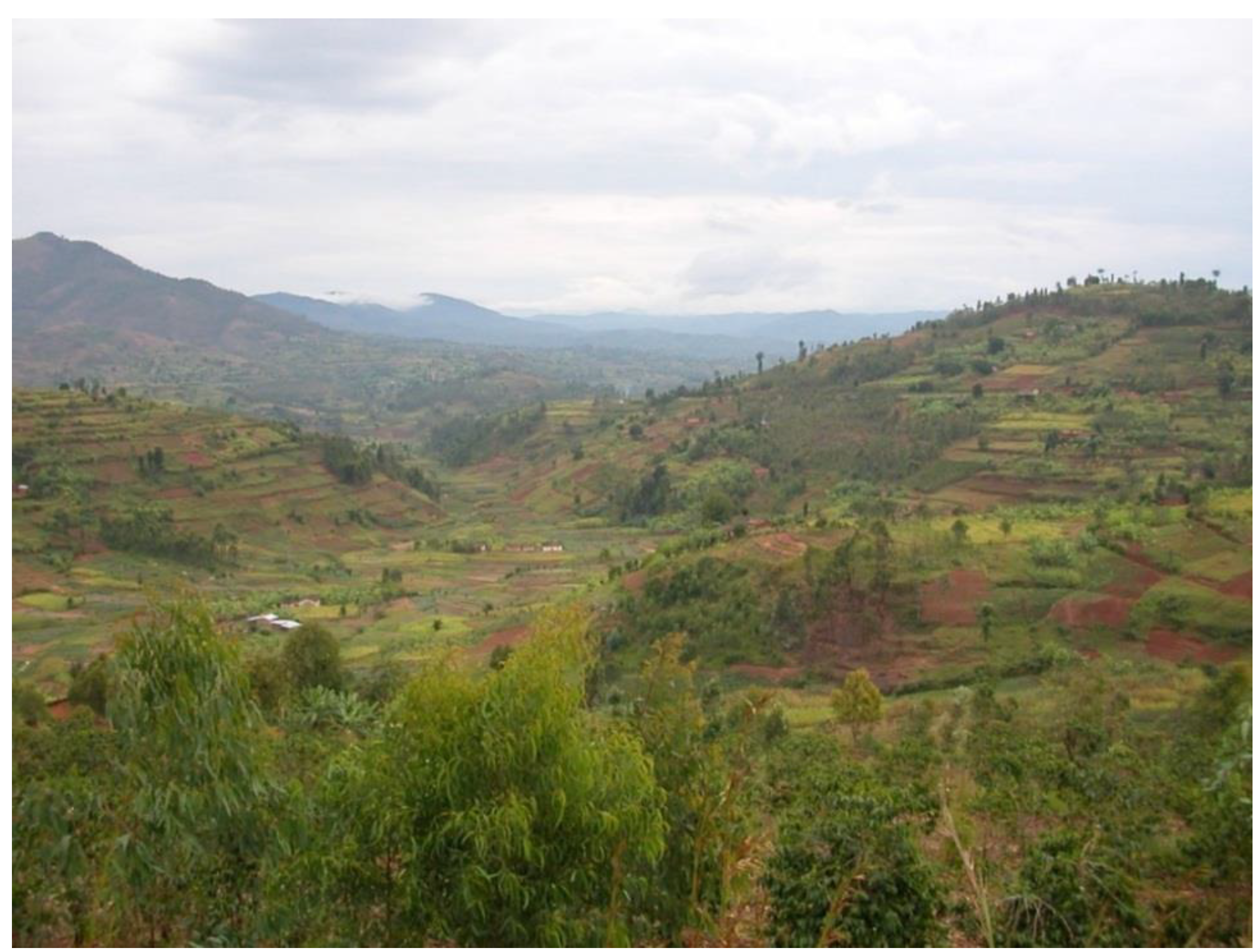
Since LEDAPS processing of Landsat imagery does not include terrain correction, topographic correction was needed to compensate for the very significant terrain illumination effects for the study region. Steep hill and mountain slopes severely affect remote sensing of vegetation. Topography results in shadowed slopes facing away from the sun and brighter slopes facing towards the sun [55,56]. This variation in illumination due to the position of the sun at the time of image acquisition and angle of the terrain is identified as the topographic illumination effect. These topographic illumination effects results in significant variation in the observed spectral characteristics of land cover for similar terrain features [57]. Therefore, topographic correction has become one of the important image preprocessing steps in the application of remote sensing data for land cover change studies in mountainous areas [58]. Many methods exist to reduce topographic illumination effects for Landsat images [56,58,59,60,61]. Vanonckelen et al. (2013) [62] achieved high land cover classification accuracy with the combination of a pixel-based Minnaert topographic compensation with an atmospheric correction. 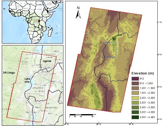Pixel based Minnaert (PBM) correction is chosen over other topographic correction methods in this study due to its higher accuracy [60]. The slope and aspect angle of the Lake Kivu region terrain were computed from the ASTER DEM as input to the terrain illumination correction for reflectance.

$${\rho }_{H,\lambda }={\rho }_{T,\lambda }\frac{\cos {\theta }_n}{{(\cos \beta \text{cos }{\theta }_n)}^{K_{\lambda }}}$$

(1)

$$cos\beta =\cos {\theta }_s\cos {\theta }_n+\sin {\theta }_s\sin {\theta }_n({\mathrm{Ø}}_t-{\mathrm{Ø}}_a)$$

(2)

Here, $K_{\lambda }$ is the slope of regression between x = log ($\text{cosβ}\cos {\theta }_n$) and y = log (${\rho }_{T,\lambda }\cos {\theta }_n)$. ${\rho }_{H,\lambda }$ is the normalized reflectance of a horizontal surface; ${\rho }_{T,\lambda }$ is the observed reflectance on an inclined terrain; β is the incident solar angle; ${\theta }_s$ is the solar zenith angle in degrees; ${\theta }_n$ is the slope angle of the terrain; ${\mathrm{Ø}}_t$ is the aspect angle of the terrain; and ${\mathrm{Ø}}_a$ is the azimuth angle in degrees.

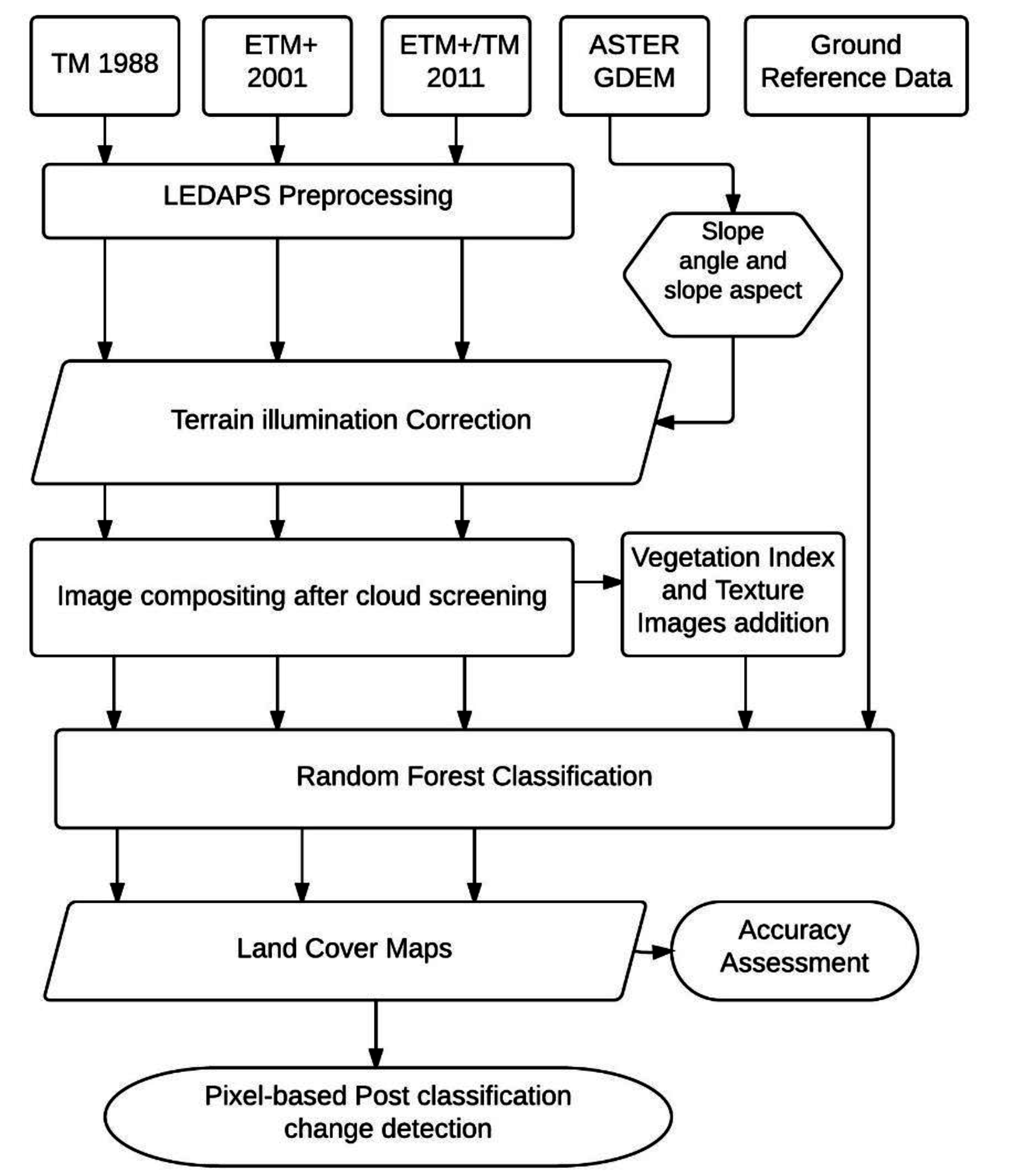
Figure 3. Flowchart for the procedures performed in the study.

Figure 3. Flowchart for the procedures performed in the study.

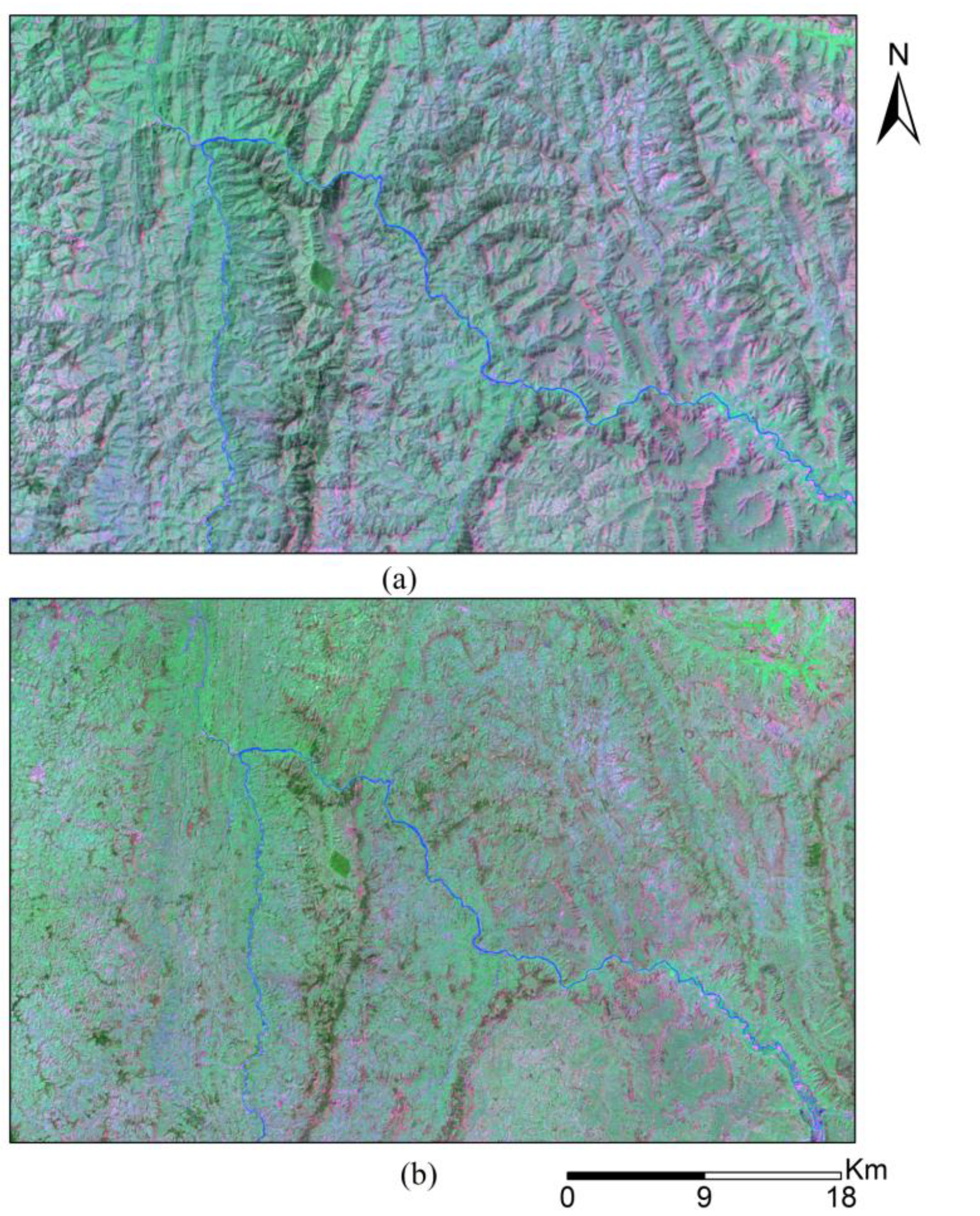
The topographic compensation was performed for all reference years (1988, 2001 and 2011). An example of the results of topographic compensation is shown in Figure 4. The shadowed slopes prominent in Figure 4a are greatly minimized in Figure 4b. This topographic compensation was an important step to minimize misclassification errors later in the process.

Figure 4. Landsat color composite (2001) of a hilly region in Rwanda (lat −1.81, lon 29.76; RGB = TM bands 7,4,2) (a) before illumination compensation; and (b) after illumination compensation.

Figure 4. Landsat color composite (2001) of a hilly region in Rwanda (lat −1.81, lon 29.76; RGB = TM bands 7,4,2) (a) before illumination compensation; and (b) after illumination compensation.

4.2. Image Compositing

To overcome the cloud cover limitations, cloud-free image composites were generated from multi-temporal image scenes covering the region [28,63,64,65]. A per-pixel based composite method was applied to remove cloud cover. The first step in the formation of a cloud-free composite was removal of cloud and cloud shadows in the Landsat scenes. A cloud-shadow mask was formed using the surface reflectance-based cloud mask, cloud shadow mask, and adjacent cloud mask provided as additional bands in the Landsat Surface Reflectance CDR product for each Landsat image. The mask was applied to the Landsat scenes to remove cloud and shadow from the scene and minimize their contamination. Since the study area is rarely cloud-free, the most cloud-free image available throughout the year was selected as the primary image for the composite. Next, imagery within ±1 year of the acquisition date of the primary image was selected to form the image composite. Finally, other image data were added to the composite until the final composite with few or no data gaps was formed. A minimum of four to a maximum of six acquisitions per target year were necessary for the composite generation. Care was given to use same season Landsat imagery, where possible, during the composite forming process. The Landsat acquisitions for each target year had an average time gap of 3 years. The list of primary Landsat acquisitions used in the study are given in Table 1.

Table 1. Primary Landsat images acquired for land cover classification in Lake Kivu region.

Landsat Sensor	Path	Row	Acquisition Date (mm/dd/yyyy)	Area Covered (km2)	Proportion in Final Composite (%)
5 TM	173	61	08/07/1987	31,756	93.79
4 TM	173	62	08/04/1989	29,761	87.98
7 ETM+	173	61	12/11/2001	29,333	85.58
7 ETM+	173	62	06/05/2002	29,183	85.16
7 ETM+	173	61	10/01/2010	24,504	69.37
5 TM	173	62	07/08/2011	18,904	53.97

Table 1. Primary Landsat images acquired for land cover classification in Lake Kivu region.

Landsat Sensor	Path	Row	Acquisition Date (mm/dd/yyyy)	Area Covered (km2)	Proportion in Final Composite (%)
5 TM	173	61	08/07/1987	31,756	93.79
4 TM	173	62	08/04/1989	29,761	87.98
7 ETM+	173	61	12/11/2001	29,333	85.58
7 ETM+	173	62	06/05/2002	29,183	85.16
7 ETM+	173	61	10/01/2010	24,504	69.37
5 TM	173	62	07/08/2011	18,904	53.97

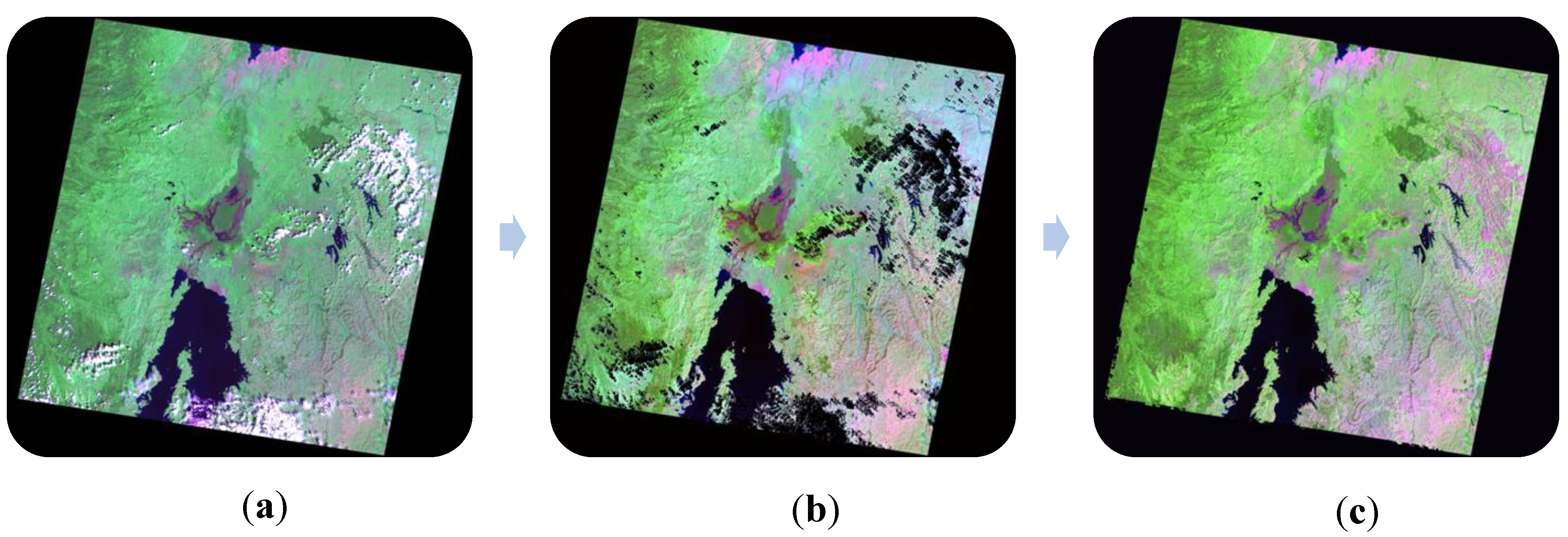
An example of the image compositing results is shown in Figure 5. Figure 5a is the primary image from 2001, with clouds at the bottom of the image and in the upper right quadrant. Figure 5b shows in black the clouds and cloud shadow mask applied in the image. Figure 5c shows the composite image where data from the other images close in time (±1 year) are used to fill the mask areas. Some areas in the region were cloudy in all images and no replacement for cloudy pixels could be done. Those regions were left with zero values (no data) for further processing. Cloud compositing was completed for all three target years 1988, 2001, and 2011.

Figure 5. Results of Landsat (RGB = TM bands 7,4,2) time composite formation for the north region (Path/Row 173/61) of the study area. (a) Primary Landsat image collected 11 December 2001; (b) after cloud and shadow removal; and (c) Landsat time composite image.

Figure 5. Results of Landsat (RGB = TM bands 7,4,2) time composite formation for the north region (Path/Row 173/61) of the study area. (a) Primary Landsat image collected 11 December 2001; (b) after cloud and shadow removal; and (c) Landsat time composite image.

4.3. Vegetation Indices and Textural Images

Selection of suitable features like vegetation indices (VI) and textural images is an important step for successful land cover classification. Textural metrics provide spatial structural information in the input data, while a vegetation index provides information to segregate vegetation from other land cover classes during classification. Rogan and Chen (2004) [66] states “To be effective, change detection approaches must maximize inter-date variance in both spectral and spatial domains (i.e., using vegetation indices and texture variables)”. Based on the work by Lu et al. (2011) [67], we used two vegetation indices, TC2 and ND42-57 (Table 2) and two textural images TM2-DIS and TM4-DIS (dissimilarity based on Thematic Mapper (TM) bands 2 and 4). Lu et al. (2011) [67] found these to be the best performers among other vegetation indices and textural images through extensive study of separability. They also found the combination of these VIs and texture bands with six Landsat TM bands produced the best overall land cover classification accuracy.

Table 2. Vegetation indices explained.

Vegetation Index	Equation
TC2	−0.285TM1 − 0.244TM2 − 0.544TM3 + 0.704TM4 + 0.084TM5 − 0.180TM7
ND42_57	(TM4 + TM2 − TM5 − TM7)/(TM4 + TM2 + TM5 + TM7)

Note: TC = tasseled cap transform; ND = Normalized difference. The ND number represents the TM spectral band.

Table 2. Vegetation indices explained.

Vegetation Index	Equation
TC2	−0.285TM1 − 0.244TM2 − 0.544TM3 + 0.704TM4 + 0.084TM5 − 0.180TM7
ND42_57	(TM4 + TM2 − TM5 − TM7)/(TM4 + TM2 + TM5 + TM7)

Note: TC = tasseled cap transform; ND = Normalized difference. The ND number represents the TM spectral band.

4.4. Image Classification

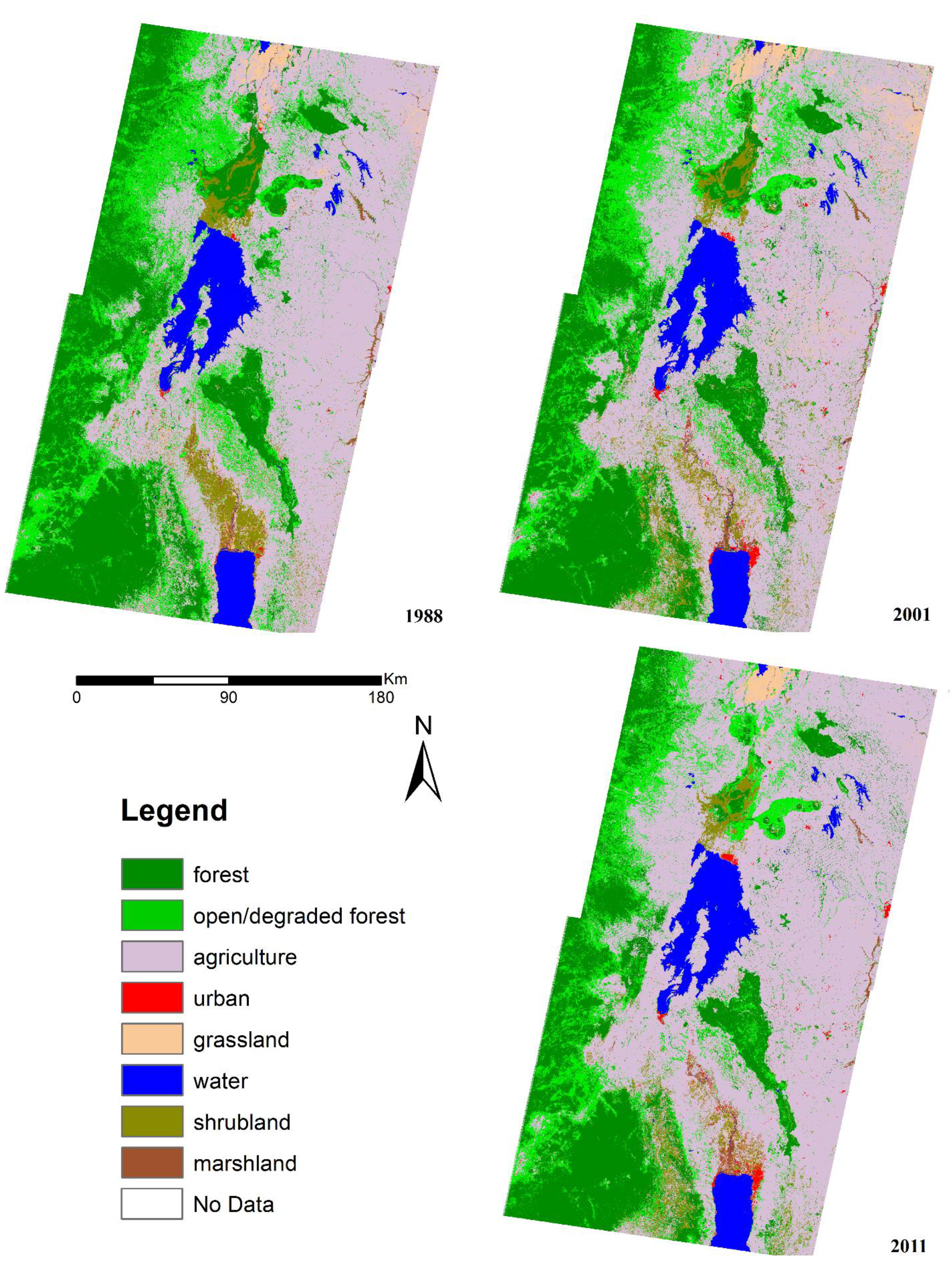
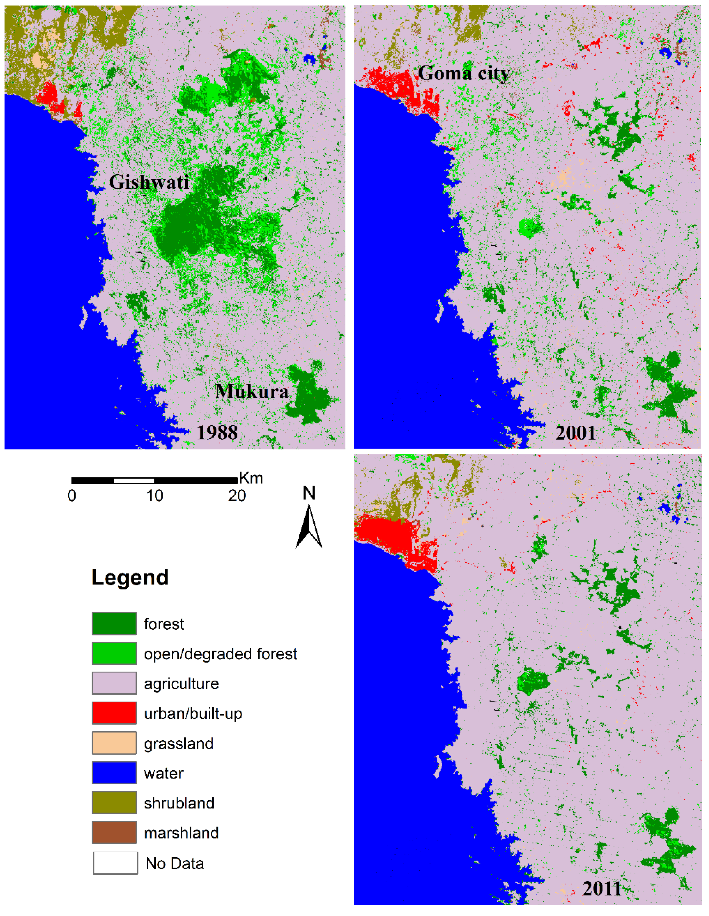
The initial step in the image classification process was to decide on the classes to be examined. Since our goal is to assess land cover change relevant to environmental processes, we implemented a categorical land cover classification system similar to the Africover land cover classes [7] with the addition of forest cover classes used by Potapov et al. (2012) [8]. Table 3 lists the eight broad land cover classes that were assessed: forest, open/degraded forest, agriculture, urban, shrubland, water, grassland, and marshland.

Table 3. Description of the land cover classes for this study.

Class	Description (Land Use Type)
Forest	Closed forest with 65% or greater canopy and height >5 m; Deciduous, evergreen and mixed forest types.
Open/degraded forest	Open forest (canopy cover from 10% to 65%) with open to close shrubs; degraded forest.
Agriculture	Areas cultivated with crops such as beans, sorghum, banana, tea, rice, maize, and other seasonal plantations; Pasturelands.
Urban	Residential, commercial services, industrial, transportation, roads, built-up land and settlement in villages.
Grassland	Areas with annual and perennial grasses.
Water	Permanent open water (100% cover), natural lakes, reservoirs and streams
Shrubland	Open general shrubs (height 0.5–5 m) with scattered herbaceous and sparse trees in between.
Marshland	Mix of water, herbaceous plants and vegetation; Swamps.

Table 3. Description of the land cover classes for this study.

Class	Description (Land Use Type)
Forest	Closed forest with 65% or greater canopy and height >5 m; Deciduous, evergreen and mixed forest types.
Open/degraded forest	Open forest (canopy cover from 10% to 65%) with open to close shrubs; degraded forest.
Agriculture	Areas cultivated with crops such as beans, sorghum, banana, tea, rice, maize, and other seasonal plantations; Pasturelands.
Urban	Residential, commercial services, industrial, transportation, roads, built-up land and settlement in villages.
Grassland	Areas with annual and perennial grasses.
Water	Permanent open water (100% cover), natural lakes, reservoirs and streams
Shrubland	Open general shrubs (height 0.5–5 m) with scattered herbaceous and sparse trees in between.
Marshland	Mix of water, herbaceous plants and vegetation; Swamps.

The next step in the process was to choose a suitable image classification method. We used the Random Forests (RF) classification in this study, which has demonstrated excellent performance for the analysis of different remote sensing datasets [68,69,70]. Random Forest, first developed by Breiman (2001) [71], is an ensemble method for supervised classification and regression based on classification and regression trees (CART). Its main advantage is the non-parametric nature, which does not require data to follow a particular distribution like normal as in case of maximum likelihood classification. Waske et al. (2009) [72] found Random Forest classifier outperforming traditional classifiers, namely single decision tree and Maximum Likelihood Classification by improved accuracy of more than 10%. RF works on the robust idea of combining outputs from more than one classifier to improve its accuracy. RF does not overfit, is less sensitive to noise, relatively quick compared to other classification methods like boosting [71] and better adapted for large datasets [73]. Compared to larger number of parameters required for other machine learning methods, the RF classifier has only two parameters: the number of trees (T) to grow the whole forest and the number of randomly selected variables (M) chosen as each split. Two methods are used to calculate M in Random Forest, one-third or square root of the number of input variables [70]. 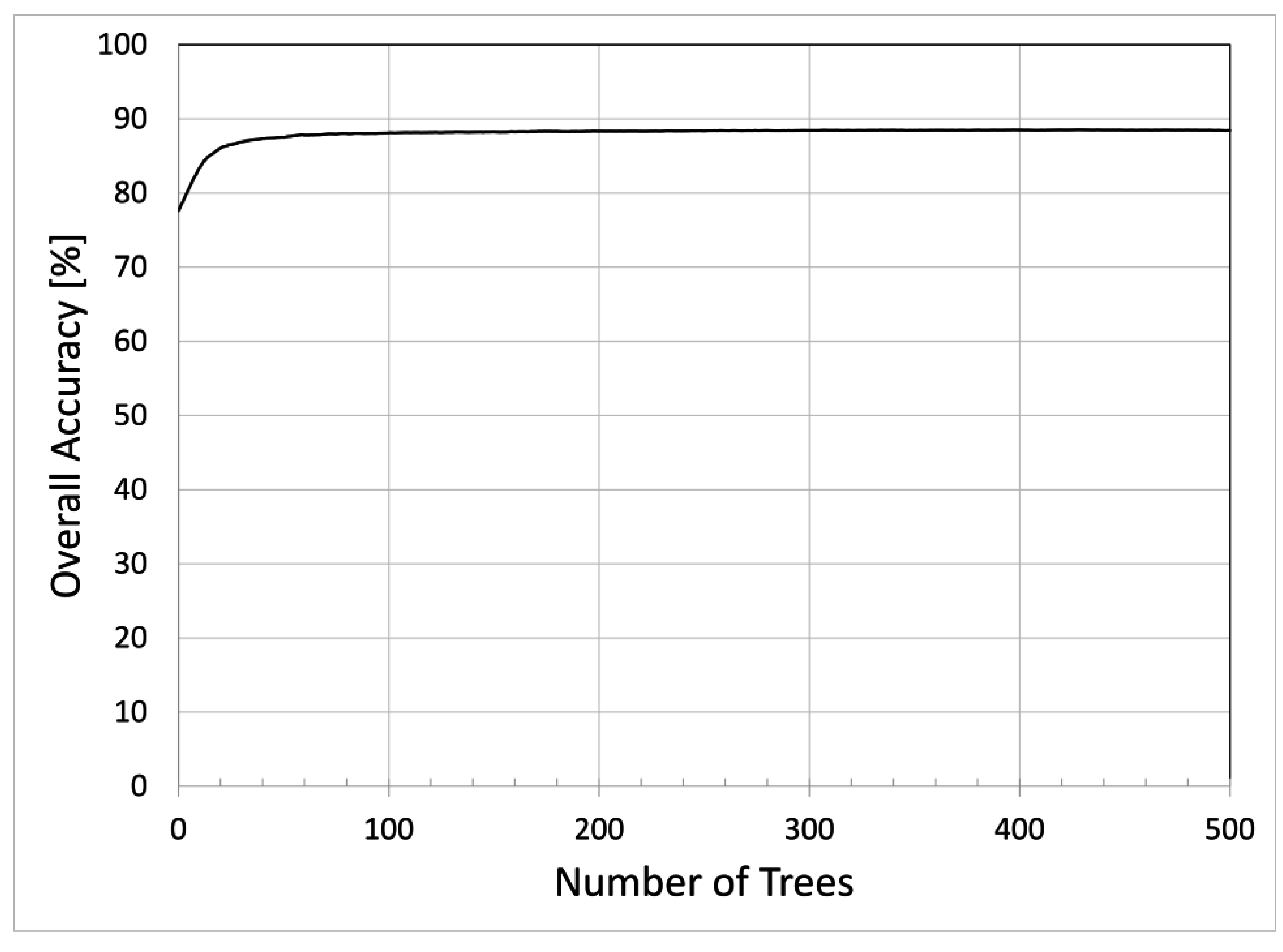Only two-third of random samples were chosen as training set and remaining one-third samples, called Out-of-Bag (OOB) samples, are used as test samples to compute classification accuracy [69]. This OOB accuracy is generally plotted against the increment of number of trees to determine appropriate number of trees. Random Forest can also measure the importance of each input variable, which indicates the contribution to classification accuracy. The RF classifier was implemented using ENVI/IDL and the EnMAP-Box software [74].

Since RF is a supervised classification method, it needs training samples for land cover classification and validation samples for accuracy assessment. Even small amounts of error in the selection of ground selection data can introduce large errors in the land cover change study [75]. Stehman and Wickham (2011) [76] argue although a universally best spatial assessment does not exist, the choice of spatial unit has broad implications on the accuracy assessment result. We used the polygon-based training data method suggested by Chen and Stow (2002) [77] for regions with heterogeneous land cover. An extensive ground reference sample set with each sample size of 7 × 7 pixels was manually selected for all land cover classes separately for each target year 1988, 2001, and 2011 by careful visual inspection of available ground reference data. The reference samples were randomly selected to avoid over- or underestimation of the spectral signature of the land cover [78]. Visual interpretation of composite Landsat imagery was required for regions where reference data of fine resolution images were not available for that time, namely 1988. Classes covering large regions of the test area were represented by approximately 261 observations (261 7 × 7 samples), while classes covering small regions were represented by a minimum of 30 observations (30 7 × 7 samples) [78,79]. The reference sample was then randomly divided in two: one for classification training and other for validation. This was done to make sure training data were spatially independent from the test data. RF was implemented using the reference training sample set in ENVI 4.7. Landsat TM Bands (1–5 and 7), two vegetation indices (TC2 and ND42-57) and two textural images (TM2-DIS and TM4-DIS) were used as input data during the classification process. As a post-classification operation, a 3 × 3 majority filter was applied to the classified maps [80] to smooth the classified images and only show the dominant classes. This process helped to reduce salt-and-pepper effects in final classification maps due to complexity of the land cover.

The output of the RF classifier exhibited significant confusion between marshland and open/degraded forest, with some of the marshland class occurring on upland sites. To compensate for this, a slope gradient map was created from the ASTER DEM and used as a mask. Marshland class pixels occurring at less than 5 degrees slope were retained while marshland class pixels at sites with greater than 5 degrees slope were converted to open/degraded forest.

4.5. Classification Accuracy and Land Cover Change Assessment

Next, the final results of land cover classification were used for accuracy assessment. Accuracy refers to degree of ‘correctness’ of a thematic map or classification [10]. Accuracy assessment refers to the extent of correspondence between remote sensing data and reference information and is based on confusion matrices using producer’s accuracy, user’s accuracy for each class, overall accuracy and the Kappa statistic for each classification scenario [81,82]. The user’s accuracy is the probability of any classified pixel to represent the correct class and the producer’s accuracy is the probability that a pixel of a known class is classified into a correct class [81]. Kappa coefficient measures the overall agreement between reference data and the classified thematic map and is considered to be a better indicator of accuracy [58,83]. The previously described validation data set was used for the accuracy assessment.

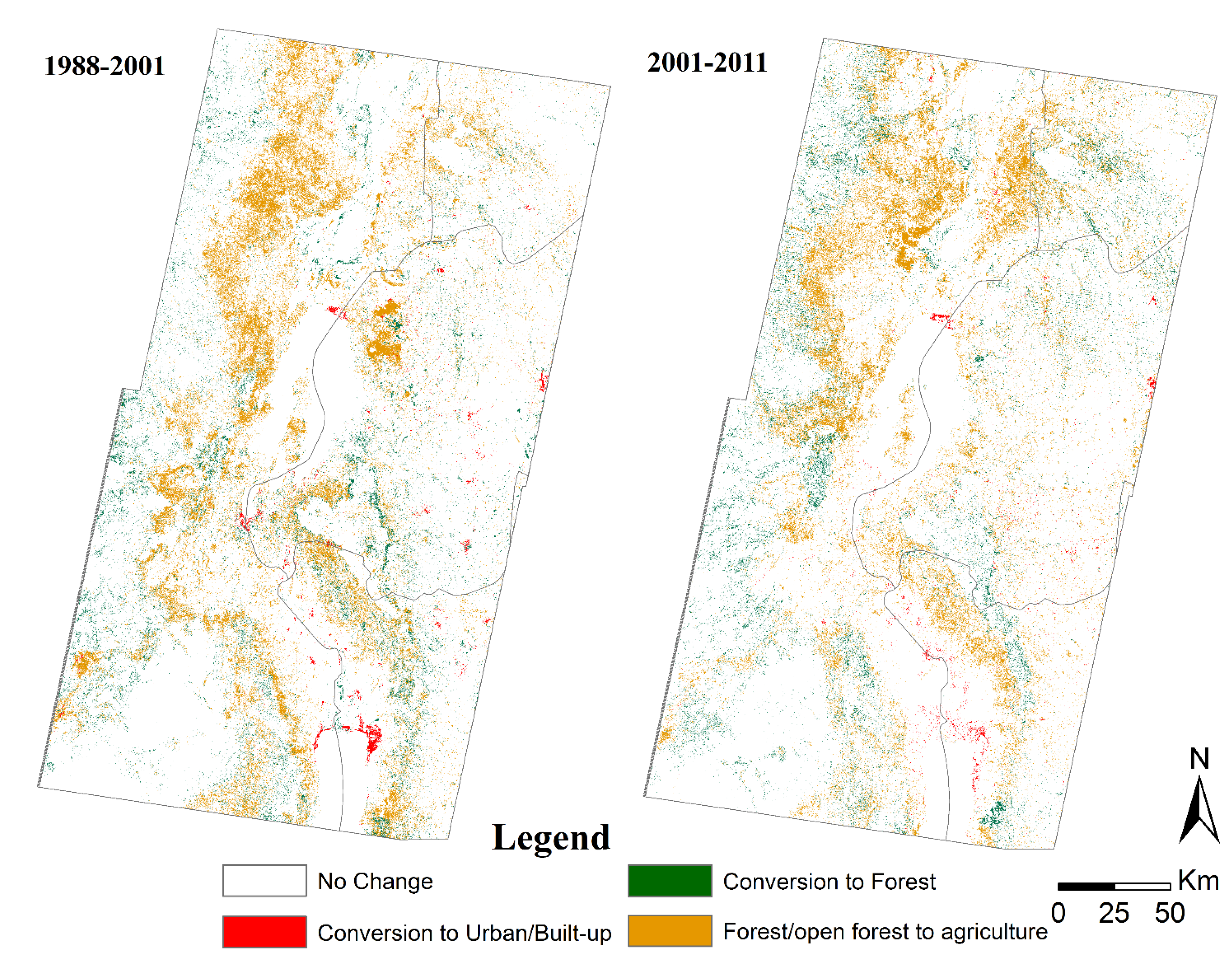
Change detection is the process of identifying differences in the state of an object or phenomenon by observing it at different times [84]. The post classification change detection method produces not only change maps as do pre-classification methods, but it also identifies the nature (from-to) of change of land cover [14,85]. These methods use separate classification of images acquired at different times and quantifies the different types of change between those intervals [15]. Land cover change assessment was performed using pixel based post-classification change detection algorithm. The most popular approach of post-classification change detection is bi-temporal change analysis of classified maps [86]. This technique was used to determine land cover change in the region for three intervals, 1988–2001, 2001–2011 and 1988–2011. ENVI 4.7 software was used to obtain the change detection results.

5. Results and Discussions

5.1. Classification Performance

To determine appropriate number of trees for RF classifier, the OOB accuracy was plotted against the increment of number of trees for 2001 image as shown in Figure 6. The RF achieved its maximum accuracy only after approximately 100 iterations and additional trees addition did not further improved the accuracy. Similar plots were obtained for other target year images, too. Thus, the number of trees (T) was selected to 100. M was chosen to be square root of the number of input variables [69].

Figure 6. Learning curve (out-of-bag-accuracy) for 2001 image.

Figure 6. Learning curve (out-of-bag-accuracy) for 2001 image.

Random Forest classification performed well in the complex landscape of Lake Kivu region with its heterogeneous environment. The addition of vegetation indices and textural images derived from Landsat, as described in Section 4, were important to the overall classification accuracy. The final overall classification accuracy ranged between 90.9% and 94.5% for the three target dates (Table 4). The Kappa coefficients ranged from 0.88 to 0.92. Thus, the overall classification accuracies were higher than the 85% minimum threshold, set by Anderson et al. [87,88] and per-class accuracy were greater than 70% [88]. Among class specific accuracies, forest, which is an important class for environmental monitoring, had producer’s and user’s accuracy better than 97% and 90%, respectively. Water class had the highest accuracy, averaging 98% due to its distinct spectral signature. The urban region (71.28%) and agriculture (73.9%) had the lowest user’s accuracy and producer’s accuracy, respectively, for 1988 map mainly due to confusion among each other. Similarly in 2001, agriculture had the lowest user’s accuracy (80%) among the classes and most errors had the shrubland misclassified as agriculture. One important factor is that agricultural plots are intimately mixed with shrubland in the hilly areas of the region causing misclassification among each other through inevitable mixed pixels. This is exacerbated by the very small farm plot sizes existing throughout this region (see Figure 2). Shrubland had the least user’s accuracy (72.2%) in the 2001 map mainly due to confusion with agriculture. Shrubland has similar spectral response with some shrub-like crops like tea and banana commonly grown in region. Grassland was the most difficult class among all to classify (average user’s accuracy 79.8% and average producer’s accuracy 90.0%) and was mostly confused with agriculture in all three target year maps.

Since agriculture and grassland with herbaceous cover have similar spectral characteristics, they were confused with each other. Further, many grasslands in this region are also used as pasturelands for agriculture, complicating the distinction among these land covers. The urban class had the average producer’s accuracy and user’s accuracy of 90% and 79%, respectively. Urban regions were mostly misclassified with agriculture during all target years in the region.

Table 4. Confusion matrices for land cover maps (in Hectares) for years 1988, 2001, and 2011.

(a) Confusion Matrix for 1988 Land Cover Map
1988	1	2	3	4	5	6	7	8	∑	UA (%)
1. Forest	926.55	32.76	0.09	0	0	0	0	0	959.4	96.58
2. Open/degraded F	20.43	348.21	65.79	0	0.18	0	2.88	10.8	448.29	77.68
3. Agriculture	0	8.73	329.49	0.09	4.32	0.27	0.54	0.81	344.25	95.71
4. Urban	0	0	9.45	61.65	7.47	0	5.76	2.16	86.49	71.28
5. Grassland	0	0	24.57	0.36	95.67	0	0.72	1.17	122.49	78.10
6. Water	0	0	0	0	0	356.85	0.27	0	357.12	99.92
7. Shrubland	0	0	1.71	1.98	5.49	0	96.03	4.32	109.53	87.67
8. Marshland	0.99	0.09	14.76	0	0.45	0	2.25	102.78	121.32	84.72
∑	947.97	389.79	445.86	64.08	113.58	357.12	108.45	122.04
PA (%)	97.74	89.33	73.90	96.21	84.23	99.92	88.55	84.22
OA (%)	90.91
Kappa	0.8839
(b) Confusion Matrix for 2001 Land Cover Map
2001	1	2	3	4	5	6	7	8	∑	UA (%)
1. Forest	1361.52	107.28	5.04	0.09	2.61	0	24.48	4.5	1505.52	90.44
2. Open/degraded F	0.18	853.65	1.62	0	1.71	0	18.72	1.62	877.5	97.28
3. Agriculture	0.09	34.11	1350.09	26.37	64.08	31.77	141.21	29.97	1677.69	80.47
4. Urban	0	0.09	0.45	421.2	1.71	0	0.18	0.9	424.53	99.22
5. Grassland	0	0.9	0.81	0.27	584.37	0	14.94	0.81	602.1	97.06
6. Water	0	0.09	0	0.18	0.9	608.94	0.36	1.08	611.55	99.57
7. Shrubland	0	13.59	1.17	0.54	10.17	0	540.63	10.08	576.18	93.83
8. Marshland	0	2.25	0.18	0.45	3.33	0.09	7.74	422.91	436.95	96.79
∑	1361.79	1011.96	1359.36	449.1	668.88	640.8	748.26	471.87
PA (%)	99.98	84.36	99.32	93.79	87.37	95.03	72.25	89.62
OA (%)	91.53
Kappa	0.9001
(c) Confusion Matrix for 2011 Land Cover Map
2011	1	2	3	4	5	6	7	8	∑	UA (%)
1. Forest	1124.8	10.17	6.48	0	0	0	0.54	0.09	1142.1	98.49
2. Open/degraded F	26.1	578.4	25.0	0	12.15	0	0	1.53	643.23	89.93
3. Agriculture	3.51	52.29	1666.3	21.42	52.65	18.36	5.4	13.41	1833.39	90.89
4. Urban	0	0	0.18	148.59	0	0	0	0	148.77	99.88
5. Grassland	0	0.09	7.02	0.27	139.9	0	0	0.09	147.42	94.93
6. Water	0	0	0	0	0	458.37	0	0.18	458.55	99.96
7. Shrubland	0	0	0	0.27	0.54	0	260.37	4.68	265.86	97.94
8. Marshland	0	0	0.63	1.17	0.27	0.09	0	187.02	189.18	98.86
∑	1154.43	640.98	1705.68	171.72	205.56	476.82	266.31	207
PA (%)	97.44	90.24	97.69	86.53	68.08	96.13	97.77	90.35
OA (%)	94.52
Kappa	92.93

Table 4. Confusion matrices for land cover maps (in Hectares) for years 1988, 2001, and 2011.

(a) Confusion Matrix for 1988 Land Cover Map
1988	1	2	3	4	5	6	7	8	∑	UA (%)
1. Forest	926.55	32.76	0.09	0	0	0	0	0	959.4	96.58
2. Open/degraded F	20.43	348.21	65.79	0	0.18	0	2.88	10.8	448.29	77.68
3. Agriculture	0	8.73	329.49	0.09	4.32	0.27	0.54	0.81	344.25	95.71
4. Urban	0	0	9.45	61.65	7.47	0	5.76	2.16	86.49	71.28
5. Grassland	0	0	24.57	0.36	95.67	0	0.72	1.17	122.49	78.10
6. Water	0	0	0	0	0	356.85	0.27	0	357.12	99.92
7. Shrubland	0	0	1.71	1.98	5.49	0	96.03	4.32	109.53	87.67
8. Marshland	0.99	0.09	14.76	0	0.45	0	2.25	102.78	121.32	84.72
∑	947.97	389.79	445.86	64.08	113.58	357.12	108.45	122.04
PA (%)	97.74	89.33	73.90	96.21	84.23	99.92	88.55	84.22
OA (%)	90.91
Kappa	0.8839
(b) Confusion Matrix for 2001 Land Cover Map
2001	1	2	3	4	5	6	7	8	∑	UA (%)
1. Forest	1361.52	107.28	5.04	0.09	2.61	0	24.48	4.5	1505.52	90.44
2. Open/degraded F	0.18	853.65	1.62	0	1.71	0	18.72	1.62	877.5	97.28
3. Agriculture	0.09	34.11	1350.09	26.37	64.08	31.77	141.21	29.97	1677.69	80.47
4. Urban	0	0.09	0.45	421.2	1.71	0	0.18	0.9	424.53	99.22
5. Grassland	0	0.9	0.81	0.27	584.37	0	14.94	0.81	602.1	97.06
6. Water	0	0.09	0	0.18	0.9	608.94	0.36	1.08	611.55	99.57
7. Shrubland	0	13.59	1.17	0.54	10.17	0	540.63	10.08	576.18	93.83
8. Marshland	0	2.25	0.18	0.45	3.33	0.09	7.74	422.91	436.95	96.79
∑	1361.79	1011.96	1359.36	449.1	668.88	640.8	748.26	471.87
PA (%)	99.98	84.36	99.32	93.79	87.37	95.03	72.25	89.62
OA (%)	91.53
Kappa	0.9001
(c) Confusion Matrix for 2011 Land Cover Map
2011	1	2	3	4	5	6	7	8	∑	UA (%)
1. Forest	1124.8	10.17	6.48	0	0	0	0.54	0.09	1142.1	98.49
2. Open/degraded F	26.1	578.4	25.0	0	12.15	0	0	1.53	643.23	89.93
3. Agriculture	3.51	52.29	1666.3	21.42	52.65	18.36	5.4	13.41	1833.39	90.89
4. Urban	0	0	0.18	148.59	0	0	0	0	148.77	99.88
5. Grassland	0	0.09	7.02	0.27	139.9	0	0	0.09	147.42	94.93
6. Water	0	0	0	0	0	458.37	0	0.18	458.55	99.96
7. Shrubland	0	0	0	0.27	0.54	0	260.37	4.68	265.86	97.94
8. Marshland	0	0	0.63	1.17	0.27	0.09	0	187.02	189.18	98.86
∑	1154.43	640.98	1705.68	171.72	205.56	476.82	266.31	207
PA (%)	97.44	90.24	97.69	86.53	68.08	96.13	97.77	90.35
OA (%)	94.52
Kappa	92.93

To compare the effect of compositing data on our classification accuracy, we closely examined the classification accuracies of the Landsat composite image for 2011. This image had the lowest percentage of primary image in the final composite (see Table 1). The classification accuracy was calculated separately for the primary image and the filled areas of the composite image. The overall classification accuracy for the primary portion of the image was 94.3%, while the overall accuracy for the filled areas of the composite image was 93.3%. These similar results suggest that our image compositing from different dates did not impact the overall classification accuracy.

5.2. Land Cover Change Assessment

5.2.1. Areas and Rates of Change

The final results of Random Forest classification for the three target years are shown in Figure 7 and the resultant land cover data are shown in Table 5. Annual change statistics for land cover in the region were also computed (Table 6). Forest in the region covered 1674 kha in 1988, 1458 kha in 2001 and 1327 kha in 2011, confirming deforestation. The annual deforestation rate for 1988–2001 period was 16.6 kha per year. This time period includes civil war (1990–1994) in Rwanda when thousands of displaced people used protected forest as sanctuaries, which is the likely cause of the greatly increased the rate of deforestation [36,42]. The end of the civil war allowed the refugees to return home through large resettlement programs reducing stress in the natural forests. The deforestation rate, as a result slowed down to 13 kha per year after 2001. The reforestation efforts in the region such as national tree planting week (implemented by Government of Rwanda) since 2001 and other environmental awareness campaigns may also have contributed to the slowdown of overall trend of deforestation, at least in Rwanda [46].

Table 5. Area and proportion of each major class during various periods in the study area (Area: kha, proportion %).

Land Cover Class	1988		2001		Area Change, 1988–2001 (kha)	2011		Area Change, 2001–2011 (kha)	Area Change, 1988–2011 (kha)
	Area (kha)	%	Area (kha)	%		Area (kha)	%
Forest	1674.7	26.81	1458.3	23.35	−216.41	1327.74	21.26	−130.58	−346.99
Open/degraded F	967.2	15.48	855.7	13.70	−111.55	771.93	12.36	−83.75	−195.30
Agriculture	2873.0	45.99	3052.8	48.87	179.81	3463.17	55.44	410.40	590.21
Urban	11.6	0.19	28.6	0.46	16.96	31.49	0.50	2.93	19.89
Grassland	93.7	1.50	177.3	2.84	83.54	62.28	1.00	−114.97	−31.44
Water	360.8	5.78	362.0	5.80	1.19	358.97	5.75	−3.05	−1.86
Shrubland	207.7	3.33	256.2	4.10	48.53	178.34	2.86	−77.87	−29.35
Marshland	57.5	0.92	55.4	0.89	−2.06	52.45	0.84	−2.99	−5.06

Table 5. Area and proportion of each major class during various periods in the study area (Area: kha, proportion %).

Land Cover Class	1988		2001		Area Change, 1988–2001 (kha)	2011		Area Change, 2001–2011 (kha)	Area Change, 1988–2011 (kha)
	Area (kha)	%	Area (kha)	%		Area (kha)	%
Forest	1674.7	26.81	1458.3	23.35	−216.41	1327.74	21.26	−130.58	−346.99
Open/degraded F	967.2	15.48	855.7	13.70	−111.55	771.93	12.36	−83.75	−195.30
Agriculture	2873.0	45.99	3052.8	48.87	179.81	3463.17	55.44	410.40	590.21
Urban	11.6	0.19	28.6	0.46	16.96	31.49	0.50	2.93	19.89
Grassland	93.7	1.50	177.3	2.84	83.54	62.28	1.00	−114.97	−31.44
Water	360.8	5.78	362.0	5.80	1.19	358.97	5.75	−3.05	−1.86
Shrubland	207.7	3.33	256.2	4.10	48.53	178.34	2.86	−77.87	−29.35
Marshland	57.5	0.92	55.4	0.89	−2.06	52.45	0.84	−2.99	−5.06

Table 6. Annual change rate of each class during various periods in the study area (positive = increase; negative = decrease; unit: kha per year).

Period	Forest	Open/Degraded Forest	Agriculture	Urban	Grassland	Water	Shrubland	Marshland
1988–2001	−16.65	−8.58	13.83	1.30	6.43	0.09	3.73	−0.16
2001–2011	−13.06	−8.38	41.04	0.29	−11.50	−0.31	−7.79	−0.30
1988–2011	−15.09	−8.49	25.66	0.86	−1.37	−0.08	−1.28	−0.22

Table 6. Annual change rate of each class during various periods in the study area (positive = increase; negative = decrease; unit: kha per year).

Period	Forest	Open/Degraded Forest	Agriculture	Urban	Grassland	Water	Shrubland	Marshland
1988–2001	−16.65	−8.58	13.83	1.30	6.43	0.09	3.73	−0.16
2001–2011	−13.06	−8.38	41.04	0.29	−11.50	−0.31	−7.79	−0.30
1988–2011	−15.09	−8.49	25.66	0.86	−1.37	−0.08	−1.28	−0.22

Open/degraded forest also depleted at a small rate (8.58 kha per year) during the period 1988–2001, and began depleting at increased rate of 8.3 kha per year after 2001. The later depletion rate coincides with increase in agriculture class during the same time period at the rate of 41.04 kha per year. This suggests open/degraded forests, the degraded version of primary forests, were mostly converted to agriculture for subsistence farming and fuel wood collection during this time. The combined forest and open/degraded forest depletion rate for 2001–2011 was 21.43 kha per year, which closely matches the rate of total forest loss found by Potapov et al., (2012) of 23.99 kha between 2001 and 2010 in combined region of Nord Kivu and Sud Kivu regions of DRC. Agriculture was the largest land cover in the region covering 2873 kha (45.9%) in 1988. Agriculture coverage increased to 48.8% in 2001 with an increase of 13.8 kha per year and later to 3463.1 kha (55%) in 2011.

Figure 7. Time series of land cover maps of the study area for 1988, 2001 and 2011.

Figure 7. Time series of land cover maps of the study area for 1988, 2001 and 2011.

The urban class was the smallest land cover in the region covering 11.6 kha (0.19%) of land area in 1988. The urban region increased by average rate of 1.3 kha per year during 1988–2001 and 0.29 kha per year after 2001. The urban region increase after 2001 may be in part due to replacement of rooftops made of natural materials with brightly reflecting metal roofs now common in the area. The areas of water in the region did not change much in the region as compared to other land cover types. The small fluctuation in water is mainly due to seasonal change in level of water in Lake Edward at the north end of the study area. The change in water may also be related to recent government programs that are in addition to the increasing fish production behind small dams and rice production. For example, rice paddy fields may be misclassified as water region during flooding season. The shrubland increased by 3.73 kha per year from 1988 to 2001, but later decreased by 7.79 kha per year from 2001 to 2011. Grassland increased during 1988–2001 period, while opposite trend happened during the 2001–2011 period. Marshland continued to decrease during the both periods. Overall both grassland and marshland decreased by average rate of 1.37 kha and 0.22 kha during the entire study period.

5.2.2. Class Change Matrices

Pixel-based post classification change detection matrices for the periods 1988–2001 and 2001–2011 are given in Table 7 and Table 8, respectively. These change matrices highlight the land cover class specific change information from one to other during the defined time frames. The individual overall classification accuracies from Table 4 were multiplied to obtain expected overall change detection accuracies of 83.2% for 1988–2001 and 86.51% for 2001–2011 [14]. From 1988 to 2001, 258.9 and 106.6 kha of forest were converted to open/degraded forest and agriculture, respectively, and 108.7 and 392.4 kha of open/degraded forest changed to forest and agriculture, respectively. Thus, the majority of forest loss was due to standing forest converting to open/degraded forest and agriculture lands. During the same time, 160.2 kha of agriculture converted to open/degraded forest, respectively. The agriculture lands during the time still increased mainly due to larger area conversion from open/degraded forest, shrubland and forest to agriculture. As a result, open/degraded forest and forest areas diminished from 1988 to 2001, as earlier reported. The urban region increased in 17 kha with major part contributed by conversion from agriculture lands (5.4 kha) while shrubland and grassland were the secondary contributors for the increase in the urban area. Construction of houses occurred in open agriculture lands to meet the demands of increasing population. It should be noted that some of the small change in areas between the land cover classes were not significant and related to classification errors.

Table 7. Matrices for land cover changes (kha) from 1988 to 2001.

2001 Area (kha)	1988
	Forest	Open/D F	Agriculture	Urban	Grassland	Water	Shrubland	Marshland
forest	1260.9	108.7	75.6	0.3	1.0	1.0	6.5	4.1
Open/D F	258.9	428.2	160.2	0.2	1.3	0.4	4.6	1.8
agriculture	106.6	392.4	2362.9	5.4	44.8	1.6	115.4	23.4
urban	0.4	1.2	13.7	4.1	1.1	0.1	7.0	0.8
grassland	0.7	3.2	132.3	0.6	34.4	0.1	4.9	1.0
water	1.3	0.6	1.5	0.1	0.3	356.4	0.3	1.5
shrubland	41.7	29.8	111.3	0.8	5.8	0.3	61.6	4.9
marshland	3.6	3.1	15.4	0.2	5.0	0.8	7.3	19.9

Table 7. Matrices for land cover changes (kha) from 1988 to 2001.

2001 Area (kha)	1988
	Forest	Open/D F	Agriculture	Urban	Grassland	Water	Shrubland	Marshland
forest	1260.9	108.7	75.6	0.3	1.0	1.0	6.5	4.1
Open/D F	258.9	428.2	160.2	0.2	1.3	0.4	4.6	1.8
agriculture	106.6	392.4	2362.9	5.4	44.8	1.6	115.4	23.4
urban	0.4	1.2	13.7	4.1	1.1	0.1	7.0	0.8
grassland	0.7	3.2	132.3	0.6	34.4	0.1	4.9	1.0
water	1.3	0.6	1.5	0.1	0.3	356.4	0.3	1.5
shrubland	41.7	29.8	111.3	0.8	5.8	0.3	61.6	4.9
marshland	3.6	3.1	15.4	0.2	5.0	0.8	7.3	19.9

Table 8. Matrices for land cover changes (kha) from 2001 to 2011.

2011 Area (kha)	2001
	Forest	Open/D F	Agriculture	Urban	Grassland	Water	Shrubland	Marshland
forest	1138.6	106.0	62.5	0.2	0.8	0.7	16.3	2.6
Open/D F	186.9	414.1	142.7	0.7	2.1	0.6	22.2	2.7
agriculture	112.6	328.0	2718.0	11.8	140.2	1.8	126.3	24.3
urban	0.3	0.4	14.4	13.4	0.5	0.1	1.1	1.2
grassland	0.5	0.7	25.8	0.6	29.4	0.4	1.8	3.0
water	0.6	0.3	0.8	0.0	0.1	356.4	0.2	0.5
shrubland	15.1	5.3	67.3	1.2	2.8	0.1	83.9	2.6
marshland	3.8	0.8	21.2	0.7	1.4	1.9	4.2	18.4

Table 8. Matrices for land cover changes (kha) from 2001 to 2011.

2011 Area (kha)	2001
	Forest	Open/D F	Agriculture	Urban	Grassland	Water	Shrubland	Marshland
forest	1138.6	106.0	62.5	0.2	0.8	0.7	16.3	2.6
Open/D F	186.9	414.1	142.7	0.7	2.1	0.6	22.2	2.7
agriculture	112.6	328.0	2718.0	11.8	140.2	1.8	126.3	24.3
urban	0.3	0.4	14.4	13.4	0.5	0.1	1.1	1.2
grassland	0.5	0.7	25.8	0.6	29.4	0.4	1.8	3.0
water	0.6	0.3	0.8	0.0	0.1	356.4	0.2	0.5
shrubland	15.1	5.3	67.3	1.2	2.8	0.1	83.9	2.6
marshland	3.8	0.8	21.2	0.7	1.4	1.9	4.2	18.4

From 2001 to 2011, 186.9 and 112.6 kha of forest were converted to open/degraded forest and agriculture, respectively, and 106.8 and 328 kha of open/degraded forest were converted to forest and agriculture, respectively. At the same time, 62.5 and 142.7 kha of agriculture converted to forest and open/degraded forests, confirming the reforestation efforts in the region. However, the reforestation area is still smaller than the total deforestation area in the region, suggesting more reforestation efforts are needed to completely reverse the trend. Agriculture continued to increase in the region at the expense of open/degraded forest, shrubland, forest, and marshland areas. A total of 11.8 and 1.2 kha of urban areas were converted to agriculture and shrubland, respectively. In Rwanda, this may be due to the settlement programs after the civil war, where scattered populations were encouraged to live close together by forming villages under a program called ‘imidugudu’. The new urban areas were built in 14.4 and 1.1 kha of agriculture and shrubland areas, respectively. There was a small decrease of Marshland during this period mainly due to conversion to agriculture.

5.2.3. Spatial Distribution of Class Change

The spatial distribution of land cover change as dynamic change maps are shown (Figure 8) for 1988–2001 and 2001–2011. Three types of change in the region were investigated: conversion to forest areas (reforestation); conversion to urban; and conversion of forest or open/degraded forest to agriculture signifying deforestation. In the 1988–2001 period, deforested areas were mostly distributed in the DRC, Gishwati Forest (Rwanda), and near Nyungwe Forest. The deforestation is mostly occurring at border areas of forest in the DRC region, which are near to human settlements. New urban regions were concentrated near the cities. Reforested areas were smaller than deforested areas.

From 2001 to 2011, reforested areas increased throughout the region as compared to earlier period. Conversion to forest can be seen in the forest in the DRC side, protected forests in Rwanda like Gishwati, Nyungwe, and Volcano National Park located north of Lake Kivu. Conversion of open/degraded forest and forests to agriculture is also prevalent in areas of high population density in the DRC region and near Nyungwe forest in Burundi. As expected, there is also an increase in urban areas near cities or towns.

Figure 8. Spatial distribution of land cover change for time period 1988–2001 and 2001–2011.

Figure 8. Spatial distribution of land cover change for time period 1988–2001 and 2001–2011.

5.3. Change Factors

Forests were depleted in the region since the start of the monitoring period in 1988. This is a great concern in the region for environment and wildlife conservation. Expansion of subsistence activities (agriculture and fuel wood collection) is the most commonly cited cause of deforestation in the Congo Basin [89]. The persistent armed conflict and genocide in 1994 [41] also caused large number of refugees migrate to forest areas and start degrading those natural resources. The civil war and refugee crisis led to great amount of forest cover loss in Gishwati Forest and Mukura Forest located in Rwanda as previously reported by Plumptre et al. (2001) [90] as shown in Figure 9. The central high region of Idjwi Island, DRC in the center of Lake Kivu is another specific region where forest was lost. Open/degraded forests depleted at the rate of 8.38 kha per year from 2001 to 2011. Similar deforestation trend in the DRC part of study region were found earlier [8]. Thus deforestation remains the major pressing change factor in the Lake Kivu region.

Forest conservation through national parks and reforestation drives are being implemented throughout the region [39]. Some of the effects are clearly visible as supported by the statistics: the rate of forest loss decreased by nearly 3 kha per year after 2001. However, open/degraded forests continue to deplete with increased rate at the same time offsetting the improvement. The region consists of developing countries and strict enforcement of conservation rules is very difficult to be implemented at ground level due to economic and political factors. Still, some progress in conservation of protected area like national parks is apparently seen in the spatial data of the region.

Figure 9. Time series of detailed land-cover maps in the study area near Goma city in Rwanda for 1988, 2001 and 2011, respectively. This mapped region is outlined in blue in Figure 1.

Figure 9. Time series of detailed land-cover maps in the study area near Goma city in Rwanda for 1988, 2001 and 2011, respectively. This mapped region is outlined in blue in Figure 1.

Agriculture has continued to expand since 1988 at the average rate of 25 kha per year. The main driving force for agriculture expansion would appear to be the population increase in the region. The population in Rwanda, Burundi and Uganda increased by 58%, 80% and 115%, respectively, during the study period, based on the census data from World Bank [91]. Since most of the population in the region is dependent on subsistence farming for their livelihood, the increase in population required creation of more agriculture lands. This in turn created stress to natural resources like forest and open/degraded forest resulting in deforestation. Currently in Rwanda, over 90 percent of the population relies on subsistence agriculture to meet their needs putting great pressure on the country’s remaining natural ecosystems. This pattern is similar to other countries of the region. The increase of agriculture lands can be good for the economy in the short-term due to increase in agriculture output, but cannot be sustained the long-term due to limited land area. Since subsistence agriculture practices in the region are mainly dependent on climatic conditions, making them vulnerable to climate change in future, the success of conservation efforts may rely in part on increases in the crop productivity and sustainable land use planning [37].

Built-up expansion in the region increased rapidly at rate of 1.3 kha per year from 1988 to 2001, which is consistent with the trend of urbanization [24] around the world. Major factor in urbanization was also the increase in population in the region and these population using forests and open/degraded forests resources to meet their livelihood causing in deforestation. Urban population in Rwanda, Burundi and Uganda were increased by 647%, 238% and 210%, respectively, during the study time based on the World Bank census data. The nature of built-up expansion in the region is also related to other factors like accessible topography and transportation.

6. Conclusions

Using multi-temporal Landsat data, we identified, quantified and analyzed decadal scale land cover change in the Lake Kivu region from 1988 to 2011. Frequent cloud coverage is a major hindrance to monitoring a tropical zone like the Lake Kivu region. Our approach employed a multi-year compositing methodology for Landsat imagery to compensate for incomplete annual data availability in the Landsat archive due to the cloud cover and other data gaps. The dominant land cover changes that took place in the study area during the study period (1988–2011) were massive deforestation, aggressive subsistence farming expansion and urban expansion. The post classification change analysis of two time intervals (1988–2001 and 2001–2011) allowed us to describe the spatial-temporal dynamics of land cover change in more detail. The change analysis found severe conversions of the natural environment as a result of human related activities. The gross forest cover loss for 1988–2001 and 2001–2011 period was 216.4 and 130.5 thousand hectares, respectively, signifying significant deforestation in the period of civil war and a relatively stable and lower deforestation rate later, due to increase in conservation and reforestation efforts in the region. Open/degraded forests were also depleted at the high rate of 8.4 kha per year over the entire period and is attributed to intensified subsistence farming.

This study demonstrates that Landsat data can provide immense insights into land cover changes over time in Central Africa despite limited data availability. However, there are limitations to the accuracy of monitoring change using Landsat data, largely due to the lack of high quality ground truth for training. However, we believe that this work will provide useful information to local land use managers in the region interested in developing ecologically sustainable land management strategies and biodiversity conservation efforts.

The land cover classification maps shown in Figure 7 are available for download as GeoTIFF images at http://www.cis.rit.edu/faculty-and-staff/profile/axvpci.

References

1. Pielke, R.A.; Pitman, A.; Niyogi, D.; Mahmood, R.; McAlpine, C.; Hossain, F.; Goldewijk, K.K.; Nair, U.; Betts, R.; Fall, S.; et al. Land use/land cover changes and climate: Modeling analysis and observational evidence. Wiley Interdiscip. Rev. Clim. Chang 2011, 2, 828–850. [Google Scholar] [CrossRef]
2. Townshend, J.; Justice, C.; Li, W.; Gurney, C.; McManus, J. Global land cover classification by remote sensing: Present capabilities and future possibilities. Remote Sens. Environ. 1991, 35, 243–255. [Google Scholar] [CrossRef]
3. Loveland, T.R.; Belward, A.S. The IGBP-DIS global 1 km land cover data set, DISCover: First results. Int. J. Remote Sens. 1997, 18, 3289–3295. [Google Scholar] [CrossRef]
4. Hansen, M.C.; Loveland, T.R. A review of large area monitoring of land cover change using Landsat data. Remote Sens. Environ. 2012, 122, 66–74. [Google Scholar] [CrossRef]
5. McGlynn, G.; Mooney, S.; Taylor, D. Palaeoecological evidence for Holocene environmental change from the Virunga volcanoes in the Albertine Rift, central Africa. Quat. Sci. Rev. 2013, 61, 32–46. [Google Scholar] [CrossRef]
6. Munyaneza, O.; Wali, U.G.; Uhlenbrook, S.; Maskey, S.; Mlotha, M.J. Water level monitoring using radar remote sensing data: Application to Lake Kivu, central Africa. Phys. Chem. Earth Parts A/B/C 2009, 34, 722–728. [Google Scholar] [CrossRef]
7. Kalensky, Z.D. AFRICOVER land cover database and map of Africa. Can. J. Remote Sens. 1998, 24, 292–297. [Google Scholar] [CrossRef]
8. Potapov, P.V.; Turubanova, S.A.; Hansen, M.C.; Adusei, B.; Broich, M.; Altstatt, A.; Mane, L.; Justice, C.O. Quantifying forest cover loss in Democratic Republic of the Congo, 2000–2010, with Landsat ETM+ data. Remote Sens. Environ. 2012, 122, 106–116. [Google Scholar] [CrossRef]
9. Elvidge, C.D.; Sutton, P.C.; Wagner, T.W. Urbanization. In Land Change Science; Gutman, G., Janetos, A.C., Justice, C.O., Moran, E.F., Mustrad, J.F., Rindfuss, R.R., Skole, D., Cochrane, M.A., Eds.; Kluwer Academic Publishers: Dordrecht, The Netherlands, 2004. [Google Scholar]
10. Foody, G.M. Status of land cover classification accuracy assessment. Remote Sens. Environ. 2002, 80, 185–201. [Google Scholar] [CrossRef]
11. Woodcock, C.E.; Allen, R.; Anderson, M.; Belward, A.; Bindschadler, R.; Coehn, W.; Gao, F.; Goward, S.N.; Helder, D.L.; Helmer, E. Free access to landsat imagery. In Science; Sills, J., Ed.; AAAS: Washington, DC, USA, 2008; Volume 320, pp. 1011–1012. [Google Scholar]
12. Helder, D.L.; Basnet, B.; Morstad, D.L. Optimized identification of worldwide radiometric pseudo-invariant calibration sites. Can. J. Remote Sens. 2010, 36, 527–539. [Google Scholar] [CrossRef]
13. Yang, X.; Lo, C.P. Using a time series of satellite imagery to detect land use and land cover changes in the Atlanta, Georgia metropolitan area. Int. J. Remote Sens. 2002, 23, 1775–1798. [Google Scholar] [CrossRef]
14. Yuan, F.; Sawaya, K.E.; Loeffelholz, B.C.; Bauer, M.E. Land cover classification and change analysis of the Twin Cities (Minnesota) Metropolitan Area by multitemporal Landsat remote sensing. Remote Sens. Environ. 2005, 98, 317–328. [Google Scholar] [CrossRef]
15. Shalaby, A.; Tateishi, R. Remote sensing and GIS for mapping and monitoring land cover and land-use changes in the Northwestern coastal zone of Egypt. Appl. Geogr. 2007, 27, 28–41. [Google Scholar] [CrossRef]
16. Dewan, A.M.; Yamaguchi, Y. Land use and land cover change in Greater Dhaka, Bangladesh: Using remote sensing to promote sustainable urbanization. Appl. Geogr. 2009, 29, 390–401. [Google Scholar] [CrossRef]
17. Bakr, N.; Weindorf, D.C.; Bahnassy, M.H.; Marei, S.M.; El-Badawi, M.M. Monitoring land cover changes in a newly reclaimed area of Egypt using multi-temporal Landsat data. Appl. Geogr. 2010, 30, 592–605. [Google Scholar] [CrossRef]
18. Ghrefat, H.A.; Goodell, P.C. Land cover mapping at Alkali Flat and Lake Lucero, White Sands, New Mexico, USA using multi-temporal and multi-spectral remote sensing data. Int. J. Appl. Earth Obs. Geoinf. 2011, 13, 616–625. [Google Scholar] [CrossRef]
19. Baumann, M.; Ozdogan, M.; Kuemmerle, T.; Wendland, K.J.; Esipova, E.; Radeloff, V.C. Using the Landsat record to detect forest-cover changes during and after the collapse of the Soviet Union in the temperate zone of European Russia. Remote Sens. Environ. 2012, 124, 174–184. [Google Scholar] [CrossRef]
20. Cohen, W.B.; Spies, T.A.; Alig, R.J.; Oetter, D.R.; Maiersperger, T.K.; Fiorella, M. Characterizing 23 Years (1972–1995) of stand replacement disturbance in western oregon forests with Landsat imagery. Ecosystems 2002, 5, 122–137. [Google Scholar] [CrossRef]
21. Li, J.; Yang, X.; Jin, Y.; Yang, Z.; Huang, W.; Zhao, L.; Gao, T.; Yu, H.; Ma, H.; Qin, Z.; et al. Monitoring and analysis of grassland desertification dynamics using Landsat images in Ningxia, China. Remote Sens. Environ. 2013, 138, 19–26. [Google Scholar] [CrossRef]
22. Ottinger, M.; Kuenzer, C.; Liu, G.; Wang, S.; Dech, S. Monitoring land cover dynamics in the Yellow River Delta from 1995 to 2010 based on Landsat 5 TM. Appl. Geogr. 2013, 44, 53–68. [Google Scholar] [CrossRef]
23. Maman, S.; Orlovsky, L.; Blumberg, D.G.; Berliner, P.; Mamedov, B. A landcover change study of takyr surfaces in Turkmenistan. J. Arid Environ. 2011, 75, 842–850. [Google Scholar] [CrossRef]
24. Taubenböck, H.; Esch, T.; Felbier, A. Monitoring urbanization in mega cities from space. Remote Sens. Environ. 2012, 117, 162–176. [Google Scholar] [CrossRef]
25. Lu, D.; Weng, Q. Spectral mixture analysis of the urban landscape in Indianapolis with Landsat ETM+ imagery. Photogramm. Eng. Remote Sens. 2004, 70, 1053–1062. [Google Scholar] [CrossRef]
26. Guerschman, J.P.; Paruelo, J.M.; di Bella, C.; Giallorenzi, M.C.; Pacin, F. Land cover classification in the Argentine Pampas using multi-temporal Landsat TM data. Int. J. Remote Sens. 2003, 24, 3381–3402. [Google Scholar] [CrossRef]
27. Röder, A.; Udelhoven, T.; Hill, J.; del Barrio, G.; Tsiourlis, G. Trend analysis of Landsat-TM and -ETM+ imagery to monitor grazing impact in a rangeland ecosystem in Northern Greece. Remote Sens. Environ. 2008, 112, 2863–2875. [Google Scholar] [CrossRef]
28. Ju, J.; Roy, D.P. The availability of cloud-free Landsat ETM+ data over the conterminous United States and globally. Remote Sens. Environ. 2008, 112, 1196–1211. [Google Scholar] [CrossRef]
29. Basnet, B.; Vodacek, A. Monitoring the dynamics of land cover in the Lake Kivu region using multi-temporal Landsat imagery. In Proceedings of the IEEE International Geoscience and Remote Sensing Symposium (IGARSS 2014 ), Quebec, QC, Canada, 13–18 July 2014; pp. 4250–4253.
30. Huang, C.; Goward, S.N.; Schleeweis, K.; Thomas, N.; Masek, J.G.; Zhu, Z. Dynamics of national forests assessed using the Landsat record: Case studies in eastern United States. Remote Sens. Environ. 2009, 113, 1430–1442. [Google Scholar] [CrossRef]
31. Kennedy, R.E.; Yang, Z.; Cohen, W.B. Detecting trends in forest disturbance and recovery using yearly Landsat time series: 1. LandTrendr—Temporal segmentation algorithms. Remote Sens. Environ. 2010, 114, 2897–2910. [Google Scholar] [CrossRef]
32. Cohen, W.B.; Yang, Z.; Kennedy, R. Detecting trends in forest disturbance and recovery using yearly Landsat time series: 2. TimeSync—Tools for calibration and validation. Remote Sens. Environ. 2010, 114, 2911–2924. [Google Scholar] [CrossRef]
33. Arvidson, T.; Goward, S.; Gasch, J.; Williams, D. Landsat-7 long-term acquisition plan: Development and validation. Photogramm. Eng. Remote Sens. 2006, 72, 1137–1146. [Google Scholar] [CrossRef]
34. Markham, B.L.; Storey, J.C.; Williams, D.L.; Irons, J.R. Landsat sensor performance: History and current status. Geosci. Remote Sens. IEEE Trans. 2004, 42, 2691–2694. [Google Scholar] [CrossRef]
35. MacKay, M.E.; Rowland, S.K.; Mouginis-Mark, P.J.; Garbeil, H. Thick lava flows of Karisimbi Volcano, Rwanda: Insights from SIR-C interferometric topography. Bull. Volcanol. 1998, 60, 239–251. [Google Scholar] [CrossRef]
36. Kanyamibwa, S. Impact of war on conservation: Rwandan environment and wildlife in agony. Biodivers. Conserv. 1998, 7, 1399–1406. [Google Scholar] [CrossRef]
37. Verdoodt, A.; van Ranst, E. Environmental assessment tools for multi-scale land resources information systemsA case study of Rwanda. Agric. Ecosyst. Environ. 2006, 114, 170–184. [Google Scholar] [CrossRef]
38. Byers, A.C., III. Soil loss and sediment transport during the storms and landslides of May 1988 in Ruhengeri prefecture, Rwanda. Nat. Hazards 1992, 5, 279–292. [Google Scholar] [CrossRef]
39. REMA. Rwanda State of Environment and Outlook; Rwanda Environment Management Authority: Kigali, Rwanda, 2009. [Google Scholar]
40. Schutte, S.; Weidmann, N.B. Diffusion patterns of violence in civil wars. Polit. Geogr. 2011, 30, 143–152. [Google Scholar] [CrossRef]
41. Straus, S. How many perpetrators were there in the Rwandan genocide? An estimate. J. Genocide Res. 2004, 6, 85–98. [Google Scholar] [CrossRef]
42. Verpoorten, M. Detecting hidden violence: The spatial distribution of excess mortality in Rwanda. Polit. Geogr. 2012, 31, 44–56. [Google Scholar] [CrossRef]
43. Nsengiyumva, J.B. Ministry of Disaster management and Refugees Affairs, R. of R. Identification of Disaster Higher Risk Zones on Floods and Landslides in Rwanda; Unit of Research and Public Awareness: Kigali, Rwanda, 2012. [Google Scholar]
44. Roose, E.; Ndayizigiye, F. Agroforestry, water and soil fertility management to fight erosion in tropical mountains of Rwanda. Soil Technol. 1997, 11, 109–119. [Google Scholar] [CrossRef]
45. International Food Policy Research Institute. Ending hunger in Africa: Prospects for the small farmer. In IFPRI Development Strategy and Governance Division Discussion Paper 9; IFPRI: Washington, DC, USA, 2004. [Google Scholar]
46. Ndayambaje, J.D.; Mohren, G.M.J. Fuelwood demand and supply in Rwanda and the role of agroforestry. Agrofor. Syst. 2011, 83, 303–320. [Google Scholar] [CrossRef]
47. Tucker, C.J.; Grant, D.M.; Dykstra, J.D. NASA’s global orthorectified Landsat data set. Photogramm. Eng. Remote Sens. 2004, 70, 313–322. [Google Scholar] [CrossRef]
48. Masek, J.G.; Vermote, E.F.; Saleous, N.E.; Wolfe, R.; Hall, F.G.; Huemmrich, K.F.; Gao, F.; Kutler, J.; Lim, T.-K. A Landsat surface reflectance dataset for North America, 1990–2000. IEEE Geosci. Remote Sens. Lett. 2006, 3, 68–72. [Google Scholar] [CrossRef]
49. Schmidt, G.; Jenkerson, C.; Masek, J.; Vermote, E.; Gao, F. Landsat Ecosystem Disturbance Adaptive Processing System (LEDAPS) Algorithm Description; US Geolo.: Reston, Virginia, 2013. [Google Scholar]
50. Vermote, E.F.; Tanré, D.; Deuze, J.L.; Herman, M.; Morcette, J.-J. Second simulation of the satellite signal in the solar spectrum, 6S: An overview. Geosci. Remote Sens. IEEE Trans. 1997, 35, 675–686. [Google Scholar] [CrossRef]
51. Ju, J.; Roy, D.P.; Vermote, E.; Masek, J.; Kovalskyy, V. Continental-scale validation of MODIS-based and LEDAPS Landsat ETM+ atmospheric correction methods. Remote Sens. Environ. 2012, 122, 175–184. [Google Scholar] [CrossRef]
52. Puertas, O.L.; Brenning, A.; Meza, F.J. Balancing misclassification errors of land cover classification maps using support vector machines and Landsat imagery in the Maipo river basin (Central Chile, 1975–2010). Remote Sens. Environ. 2013, 137, 112–123. [Google Scholar] [CrossRef]
53. Nikolakopoulos, K.G.; Kamaratakis, E.K.; Chrysoulakis, N. SRTM vs. ASTER elevation products. Comparison for two regions in Crete, Greece. Int. J. Remote Sens. 2006, 27, 4819–4838. [Google Scholar] [CrossRef]
54. Tachikawa, T.; Kaku, M.; Iwasaki, A.; Gesch, D.; Oimoen, M.; Zhang, Z.; Danielson, J.; Krieger, T.; Curtis, B.; Haase, J.; et al. ASTER Global Digital Elevation Model Version 2—Summary of Validation Results. Available online: http://www.jspacesystems.or.jp/ersdac/GDEM/ver2Validation/Summary_GDEM2_validation_report_final.pdf (accessed on 9 February 2015).
55. Tokola, T.; Sarkeala, J.; van der Linden, M. Use of topographic correction in Landsat TM-based forest interpretation in Nepal. Int. J. Remote Sens. 2001, 22, 551–563. [Google Scholar] [CrossRef]
56. Shepherd, J.D.; Dymond, J.R. Correcting satellite imagery for the variance of reflectance and illumination with topography. Int. J. Remote Sens. 2003, 24, 3503–3514. [Google Scholar] [CrossRef]
57. Veraverbeke, S.; Verstraeten, W.W.; Lhermitte, S.; Goossens, R. Illumination effects on the differenced Normalized Burn Ratio’s optimality for assessing fire severity. Int. J. Appl. Earth Obs. Geoinf. 2010, 12, 60–70. [Google Scholar] [CrossRef]
58. Tan, B.; Masek, J.G.; Wolfe, R.; Gao, F.; Huang, C.; Vermote, E.F.; Sexton, J.O.; Ederer, G. Improved forest change detection with terrain illumination corrected Landsat images. Remote Sens. Environ. 2013, 136, 469–483. [Google Scholar] [CrossRef]
59. Teillet, P.M.; Guindon, B.; Goodenough, D.G. On the slope-aspect correction of multispectral scanner data. Can. J. Remote Sens. 1982, 8. [Google Scholar] [CrossRef]
60. Lu, D.; Ge, H.; He, S.; Xu, A.; Zhou, G.; Du, H. Pixel-based Minnaert correction method for reducing topographic effects on a Landsat 7 ETM+ image. Photogramm. Eng. Remote Sens. 2008, 74, 1343–1350. [Google Scholar]
61. Gao, Y.; Zhang, W. A simple empirical topographic correction method for ETM+ imagery. Int. J. Remote Sens. 2009, 30, 2259–2275. [Google Scholar] [CrossRef]
62. Vanonckelen, S.; Lhermitte, S.; van Rompaey, A. The effect of atmospheric and topographic correction methods on land cover classification accuracy. Int. J. Appl. Earth Obs. Geoinf. 2013, 24, 9–21. [Google Scholar] [CrossRef]
63. Lindquist, E.J.; Hansen, M.C.; Roy, D.P.; Justice, C.O. The suitability of decadal image data sets for mapping tropical forest cover change in the Democratic Republic of Congo: Implications for the global land survey. Int. J. Remote Sens. 2008, 29, 7269–7275. [Google Scholar] [CrossRef]
64. Luo, Y.; Trishchenko, A.; Khlopenkov, K. Developing clear-sky, cloud and cloud shadow mask for producing clear-sky composites at 250-m spatial resolution for the seven MODIS land bands over Canada and North America. Remote Sens. Environ. 2008, 112, 4167–4185. [Google Scholar] [CrossRef]
65. Bhattarai, N.; Quackenbush, L.J.; Dougherty, M.; Marzen, L.J. A simple Landsat-MODIS fusion approach for monitoring seasonal evapotranspiration at 30 m spatial resolution. Int. J. Remote Sens. 2014, 36, 115–143. [Google Scholar] [CrossRef]
66. Rogan, J.; Chen, D. Remote sensing technology for mapping and monitoring land-cover and land-use change. Prog. Plan. 2004, 61, 301–325. [Google Scholar] [CrossRef]
67. Lu, D.; Weng, Q.; Moran, E.; Li, G.; Hetrick, S. Remote sensing image classification. In Advances in Environmental Remote Sensing: Sensors, Algorithms, and Applications; Weng, Q., Ed.; CRC Press/Taylor and Francis: Boca Raton, FL, USA, 2011; pp. 219–240. [Google Scholar]
68. Stefanski, J.; Mack, B.; Waske, B. Optimization of object-based image analysis with random forests for land cover mapping. IEEE J. Sel. Top. Appl. Earth Obs. Remote Sens. 2013, 6, 2492–2504. [Google Scholar] [CrossRef]
69. Guo, L.; Chehata, N.; Mallet, C.; Boukir, S. Relevance of airborne lidar and multispectral image data for urban scene classification using Random Forests. ISPRS J. Photogramm. Remote Sens. 2011, 66, 56–66. [Google Scholar] [CrossRef]
70. Rodriguez-Galiano, V.F.; Chica-Olmo, M.; Abarca-Hernandez, F.; Atkinson, P.M.; Jeganathan, C. Random forest classification of Mediterranean land cover using multi-seasonal imagery and multi-seasonal texture. Remote Sens. Environ. 2012, 121, 93–107. [Google Scholar] [CrossRef]
71. Breiman, L. Random forests. Mach. Learn. 2001, 45, 5–32. [Google Scholar] [CrossRef]
72. Waske, B.; Braun, M. Classifier ensembles for land cover mapping using multitemporal SAR imagery. ISPRS J. Photogramm. Remote Sens. 2009, 64, 450–457. [Google Scholar] [CrossRef]
73. Puissant, A.; Rougier, S.; Stumpf, A. Object-oriented mapping of urban trees using Random Forest classifiers. Int. J. Appl. Earth Obs. Geoinf. 2014, 26, 235–245. [Google Scholar] [CrossRef]
74. Waske, B.; van der Linden, S.; Oldenburg, C.; Jakimow, B.; Rabe, A.; Hostert, P. ImageRF—A user-oriented implementation for remote sensing image analysis with Random Forests. Environ. Model. Softw. 2012, 35, 192–193. [Google Scholar] [CrossRef]
75. Foody, G.M. Assessing the accuracy of land cover change with imperfect ground reference data. Remote Sens. Environ. 2010, 114, 2271–2285. [Google Scholar] [CrossRef]
76. Stehman, S.V.; Wickham, J.D. Pixels, blocks of pixels, and polygons: Choosing a spatial unit for thematic accuracy assessment. Remote Sens. Environ. 2011, 115, 3044–3055. [Google Scholar] [CrossRef]
77. Chen, D.; Stow, D. The effect of training strategies on supervised classification at different spatial resolutions. Photogramm. Eng. Remote Sens. 2002, 68, 1155–1162. [Google Scholar]
78. Congalton, R.G.; Green, R. Assessing the Accuracy of Remotely Sensed Data: Principles and Practices, 2nd ed.; CRC/Taylor & Francis: Boca Raton, FL, USA, 2009. [Google Scholar]
79. Kindu, M.; Schneider, T.; Teketay, D.; Knoke, T. Land use/land cover change analysis using object-based classification approach in Munessa-Shashemene landscape of the ethiopian highlands. Remote Sens. 2013, 5, 2411–2435. [Google Scholar] [CrossRef]
80. Lillesand, T.M.; Kiefer, R.W.; Chipman, J.W. Remote Sensing and Image Interpretation, 5th ed.; John Wiley & Sons: New York, NY, USA, 2004. [Google Scholar]
81. Congalton, R.G. A review of assessing the accuracy of classifications of remotely sensed data. Remote Sens. Environ. 1991, 37, 35–46. [Google Scholar] [CrossRef]
82. Smits, P.C.; Dellepiane, S.G.; Schowengerdt, R.A. Quality assessment of image classification algorithms for land-cover mapping: A review and a proposal for a cost-based approach. Int. J. Remote Sens. 1999, 20, 1461–1486. [Google Scholar] [CrossRef]
83. Huang, C.; Goward, S.N.; Masek, J.G.; Thomas, N.; Zhu, Z.; Vogelmann, J.E. An automated approach for reconstructing recent forest disturbance history using dense Landsat time series stacks. Remote Sens. Environ. 2010, 114, 183–198. [Google Scholar] [CrossRef]
84. Singh, A. Review article digital change detection techniques using remotely-sensed data. Int. J. Remote Sens. 1989, 10, 989–1003. [Google Scholar] [CrossRef]
85. Im, J.; Jensen, J. A change detection model based on neighborhood correlation image analysis and decision tree classification. Remote Sens. Environ. 2005, 99, 326–340. [Google Scholar] [CrossRef]
86. Coppin, P.; Jonckheere, I.; Nackaerts, K.; Muys, B.; Lambin, E. Digital change detection methods in ecosystem monitoring: A review. Int. J. Remote Sens. 2004, 25, 1565–1596. [Google Scholar] [CrossRef]
87. Anderson, J.R.; Hardy, E.E.; Roach, J.T.; Witmer, R.E.; Peck, D.L. A Land Use And Land Cover Classification System for Use With Remote Sensor Data; United States Government Printing Office: Washington, DC, USA, 1976.
88. Thomlinson, J.R.; Bolstad, P.V.; Cohen, W.B. Coordinating methodologies for scaling landcover classifications from site-specific to global: Steps toward validating global map products. Remote Sens. Environ. 1999, 70, 16–28. [Google Scholar] [CrossRef]
89. Megevand, C.; Mosnier, A.; Hourticq, J.; Sanders, K.; Doetinchem, N.; Streck, C. What will drive deforestation in the Congo Basin? A multisectoral analysis. In Deforestation Trends in the Congo Basin; Directions in Development-Environment and Sustainable Development; The World Bank: Washington, DC, USA, 2013; pp. 57–118. [Google Scholar]
90. Plumptre, A.J.; Masozera, M.; Vedder, A. The Impact of Civil War on the Conservation of Protected Areas in Rwanda; Biodiversity Support Program: Washington, DC, USA, 2001. [Google Scholar]
91. The world bank. World Development Indicators Online (WDI). Available online: http://data.worldbank.org/ (accessed on 9 February 2015).