
Feature Selection of Time Series MODIS Data for Early Crop Classification Using Random Forest: A Case Study in Kansas, USA


Abstract
:
1. Introduction
2. Study Area and Datasets
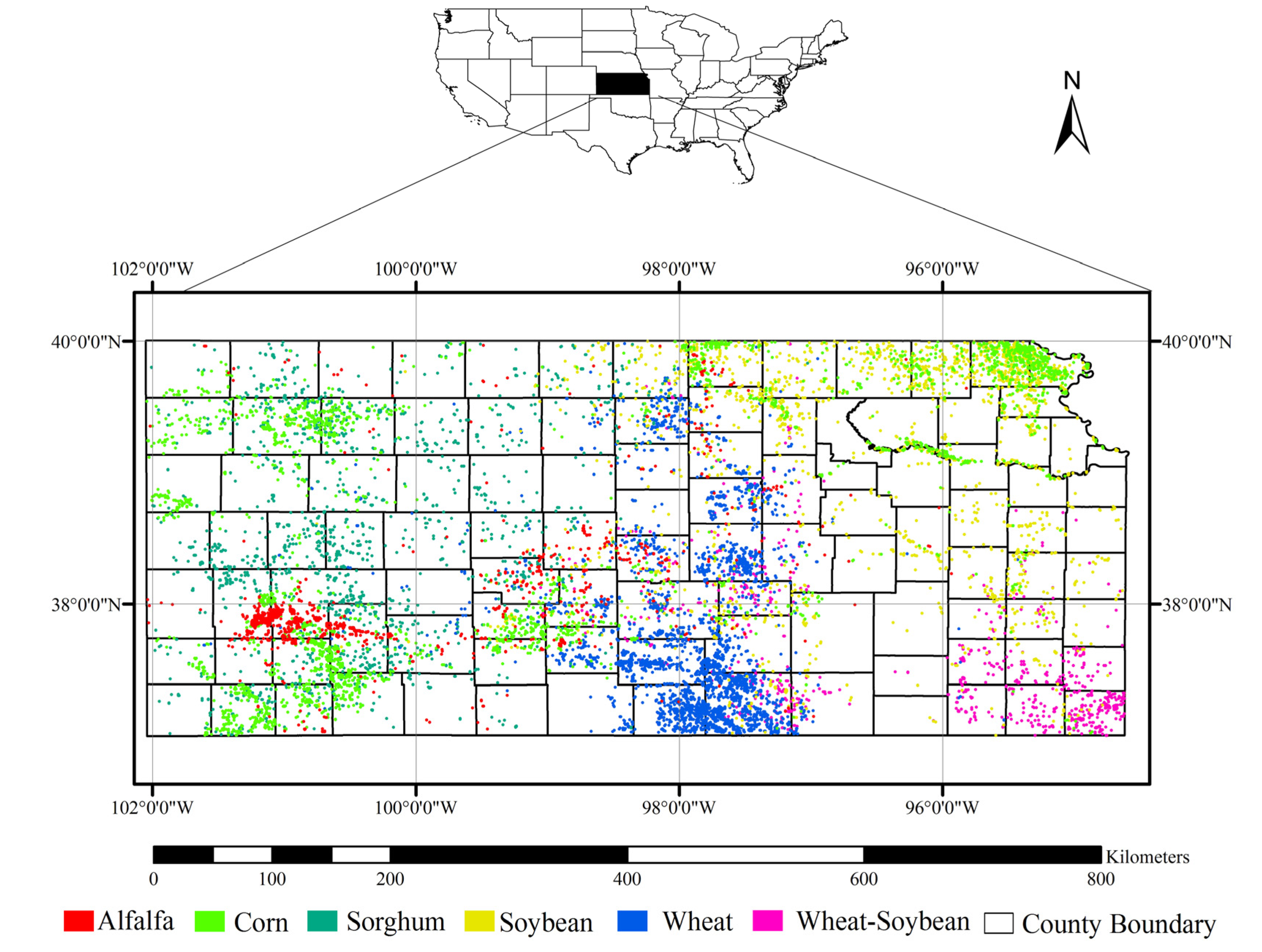
2.1. Study Area
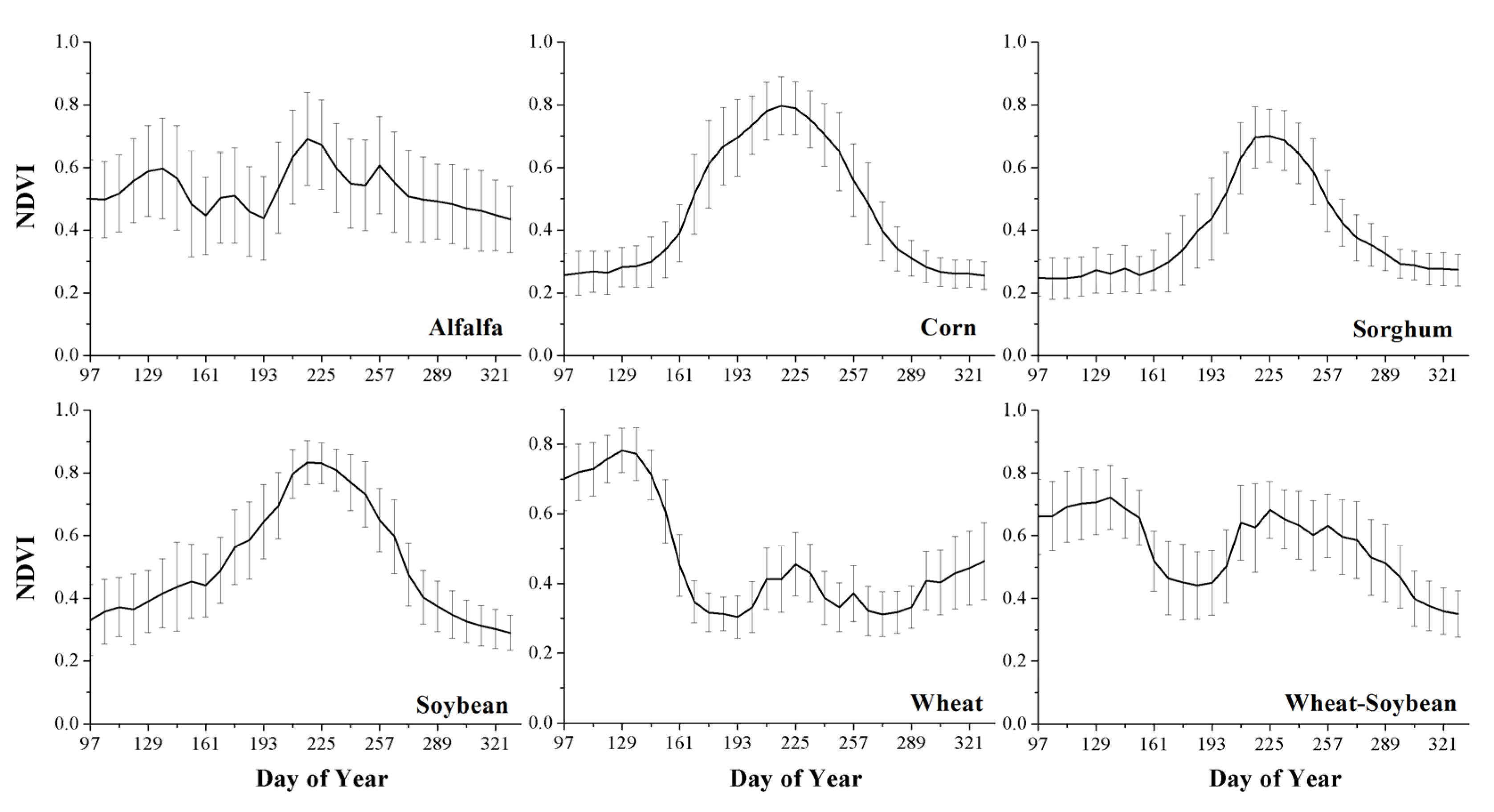
2.2. MODIS Data and Derived Phenological Variables


| Group Name | Number of Variables in the Group | Denotation of Variables |
|---|---|---|
| Reflectance | 210 (30 images ×7 bands) | BxDy, x = 1,2,…7, y = 1,2,…30 |
| Indices (NDVI and NDWI) | 60 (30 image × 2 bands) | NDVI_Dy, NDWI_Dy, y = 1,2,…30 |
| Phenological metrics | 9 | SOST, SOSN, EOST, EOSN, MaxN, MaxT, DOS, AON, TIN |
2.3. Reference Dataset
| Crop Type | CDL Code | Producer’s Accuracy | User’s Accuracy | Areal Proportions |
|---|---|---|---|---|
| Winter Wheat | 24 | 94.37% | 94.45% | 38.33% |
| Corn | 1 | 93.21% | 93.6% | 16.99% |
| Soybeans | 5 | 92.97% | 92.97% | 13.66% |
| Sorghum | 4 | 89.32% | 89.27% | 11.25% |
| Fallow/Idle Cropland | 61 | 87.47% | 87.81% | 11.02% |
| (Double Crop) Winter Wheat/Soybeans | 26 | 85.9% | 85.25% | 3.00% |
| Other Hay/Non Alfalfa | 37 | 56.07% | 90.39% | 2.85% |
| Alfalfa | 36 | 85.95% | 91.21% | 1.95% |
| (Double Crop) Winter Wheat/Sorghum | 236 | 36.64% | 65.03% | 0.37% |
| Canola | 31 | 78.22% | 90.75% | 0.12% |
| Rye | 27 | 37.55% | 76.76% | 0.11% |
| Oats | 28 | 37.63% | 72.27% | 0.10% |
| Crop Type | Training | Validation |
|---|---|---|
| Alfalfa | 562 | 561 |
| Corn | 1441 | 1441 |
| Sorghum | 847 | 847 |
| Soybean | 1005 | 1006 |
| Wheat | 1665 | 1664 |
| Wheat-soybean | 437 | 437 |
| Total | 5957 | 5956 |
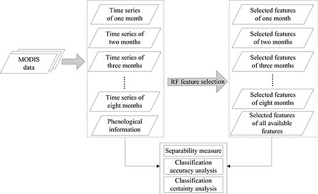
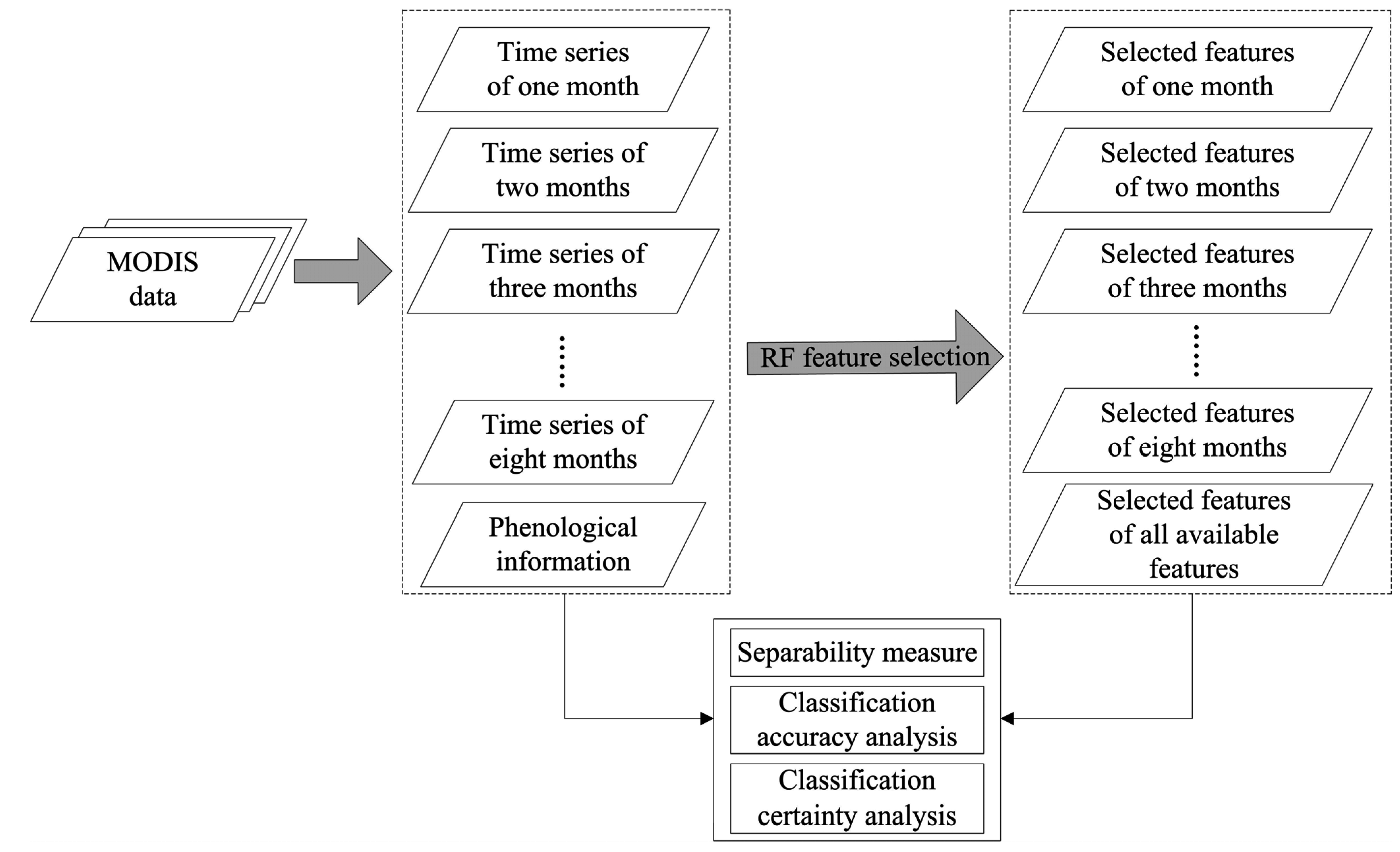
3. Method
3.1. Random Forest

3.2. Extension of the Jeffries–Matusita Distance
3.3. Accuracy and Certainty Measures
4. Results
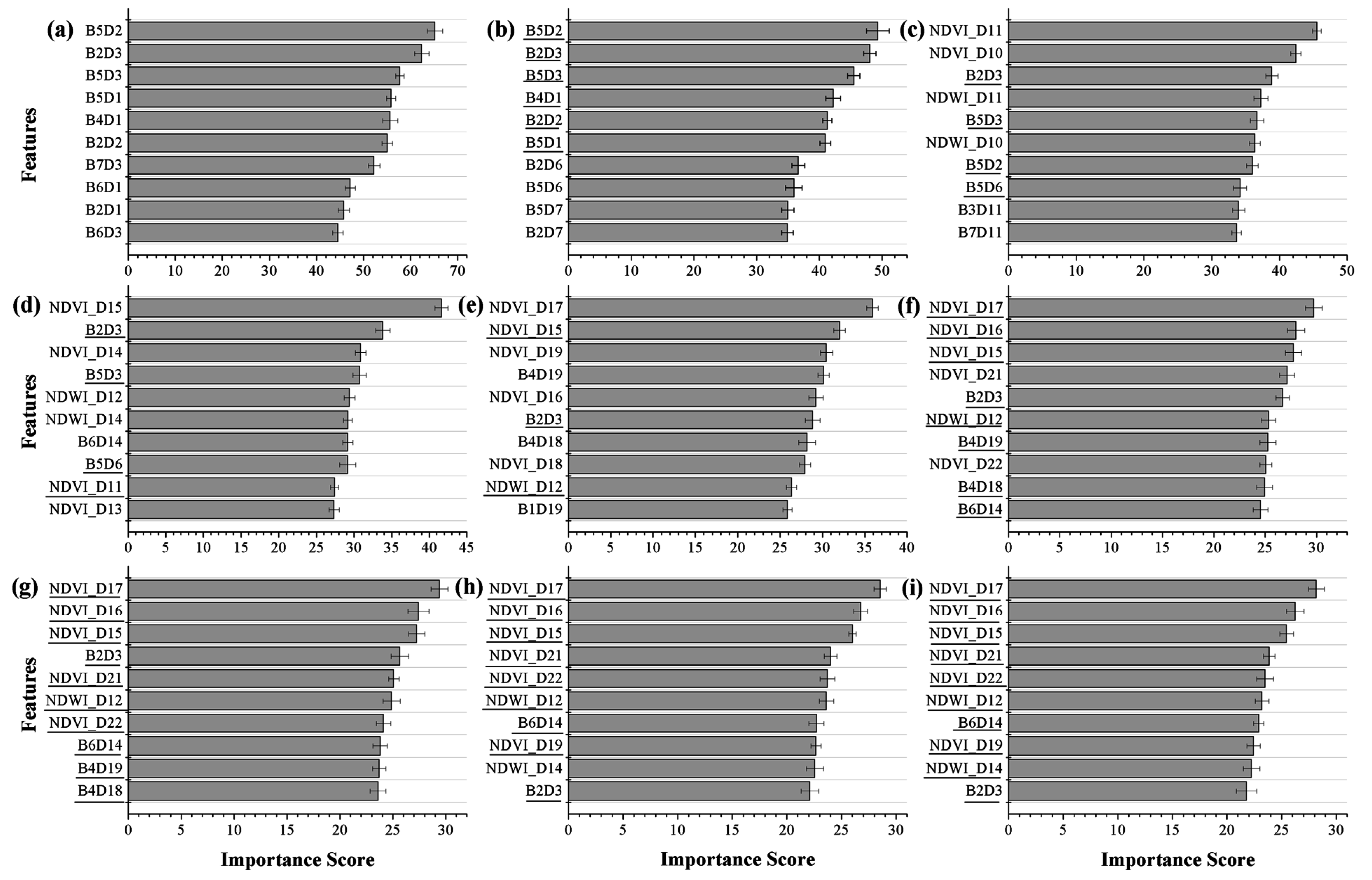
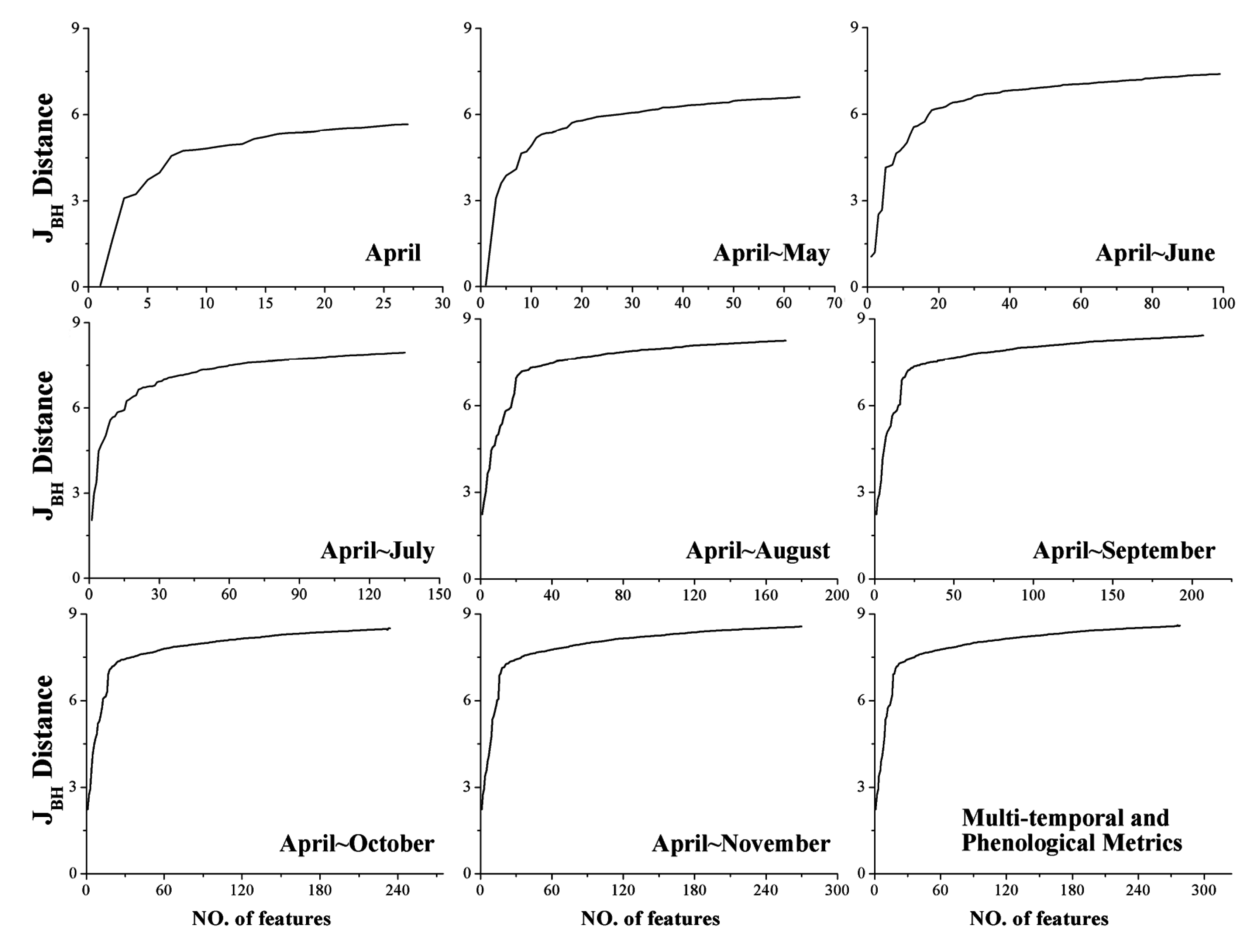
4.1. Importance of Features for Crop Mapping

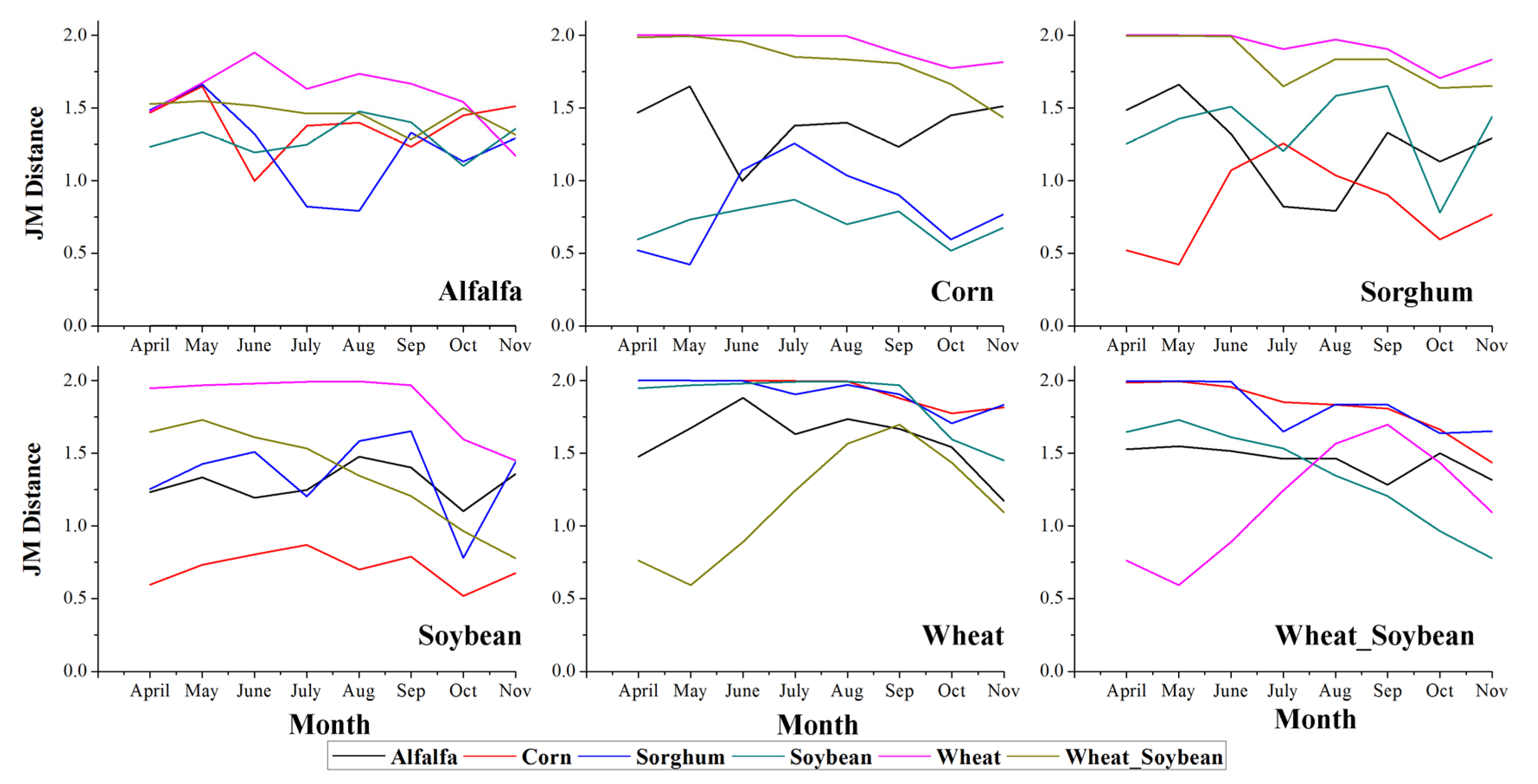
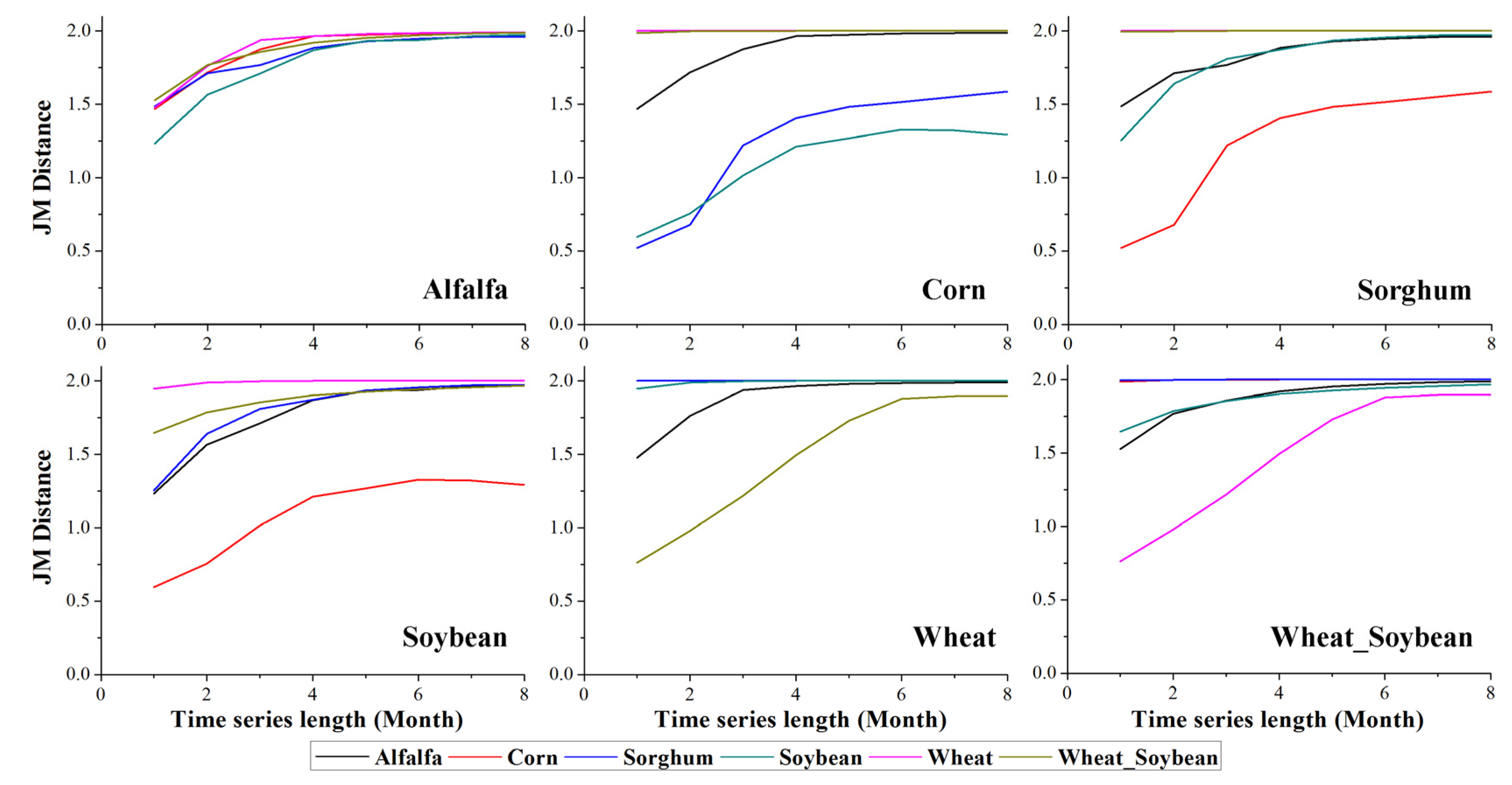
4.2. Class Separability


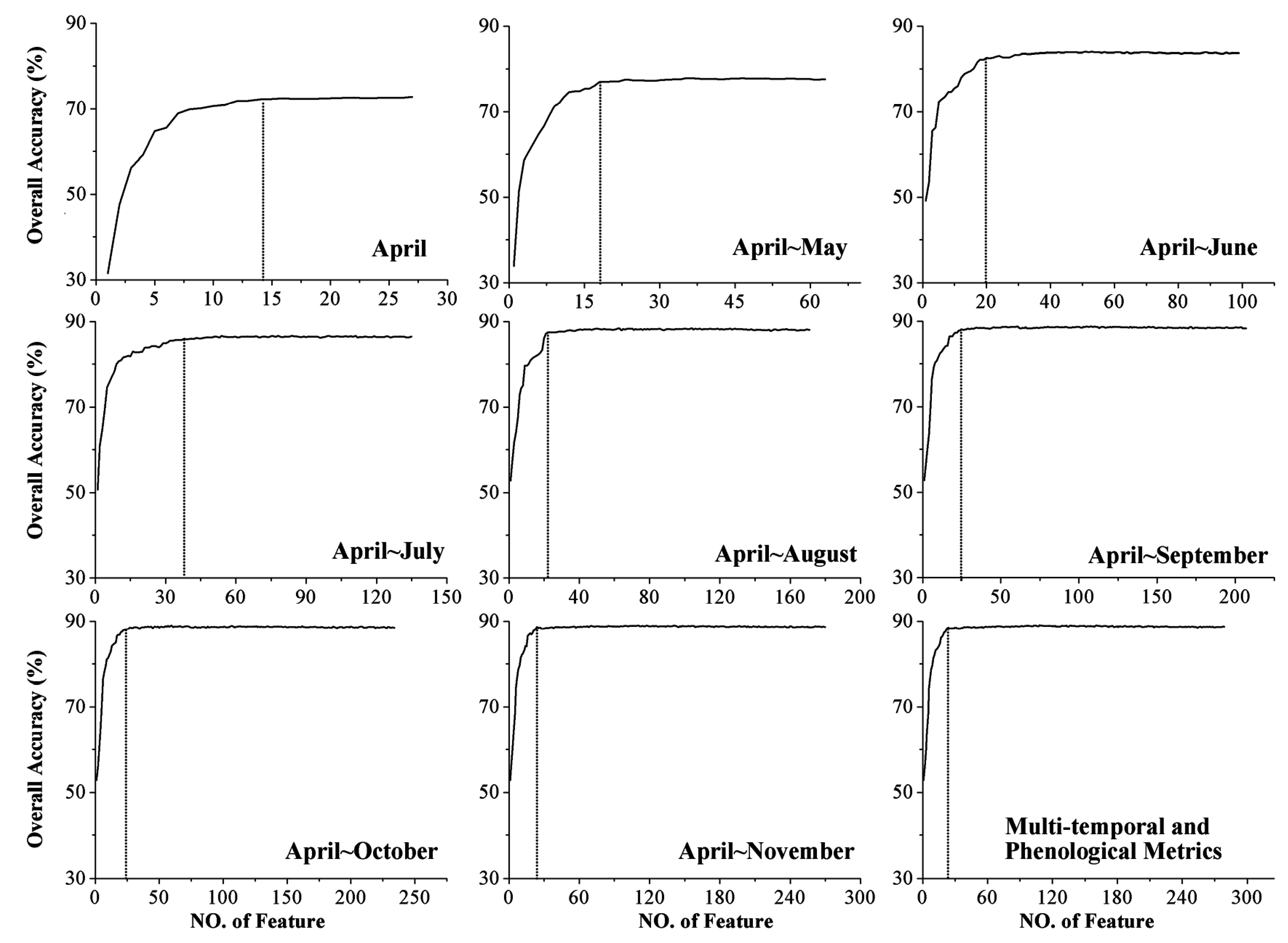
4.3. Classification Accuracy

| Alfalfa | Corn | Sorghum | Soybean | Wheat | Wheat-Soybean | |
|---|---|---|---|---|---|---|
| PA/UA | PA/UA | PA/UA | PA/UA | PA/UA | PA/UA | |
| April | 62.2%/75.9% | 70.0%/63.1% | 55.5%/67.2% | 65.7%/61.3% | 96.8%/88.0% | 56.1%/84.2% |
| April ~ May | 71.3%/87.3% | 79.3%/66.4% | 62.6%/74.5% | 66.5%/70.9% | 97.8%/88.9% | 58.4%/87.3% |
| April ~ June | 75.4%/92.4% | 83.9%/78.5% | 79.8%/81.8% | 75.8%/74.8% | 99.1%/91.3% | 61.1%/87.5% |
| April ~ July | 81.3%/92.5% | 86.1%/82.0% | 82.3%/84.0% | 78.8%/78.7% | 99.6%/93.6% | 70.3%/89.8% |
| April ~ August | 85.6%/92.1% | 86.0%/83.2% | 83.7%/87.1% | 81.8%/80.2% | 99.6%/95.4% | 76.9%/91.1% |
| April ~ September | 85.4%/92.3% | 85.8%/83.4% | 84.1%/87.3% | 82.1%/79.7% | 99.5%/96.6% | 80.8%/90.8% |
| April ~ October | 85.2%/92.1% | 86.4%/83.6% | 83.9%/87.5% | 82.1%/79.9% | 99.5%/96.7% | 81.0%/90.5% |
| April ~ November | 85.7%/93.0% | 85.7%/84.5% | 84.5%/87.1% | 82.8%/79.8% | 99.4%/96.7% | 81.0%/91.0% |
| Add Phe | 85.6%/93.3% | 85.9%/84.2% | 84.2%/87.5% | 83.2%/79.6% | 99.5%/96.5% | 81.0%/91.1% |
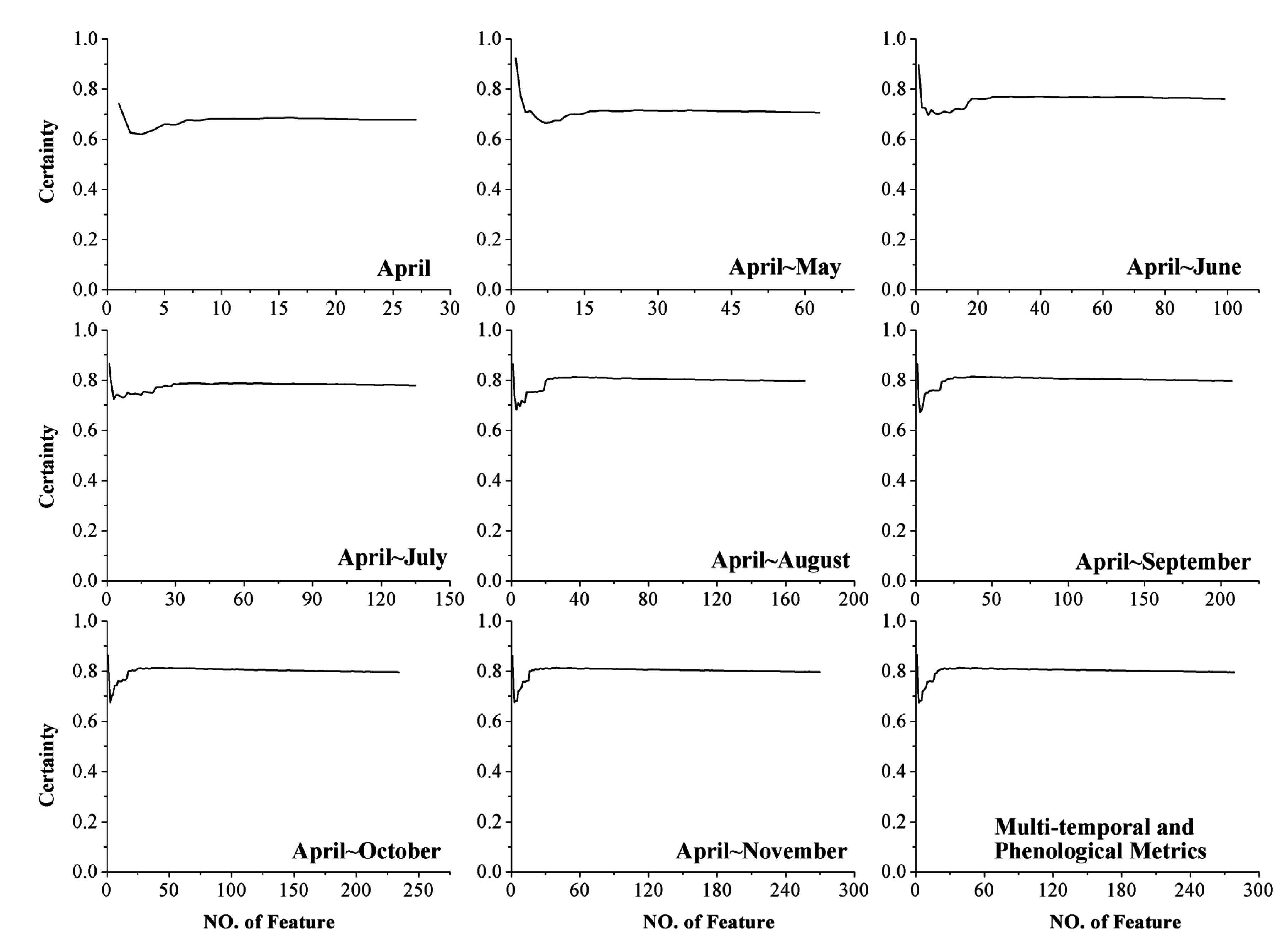
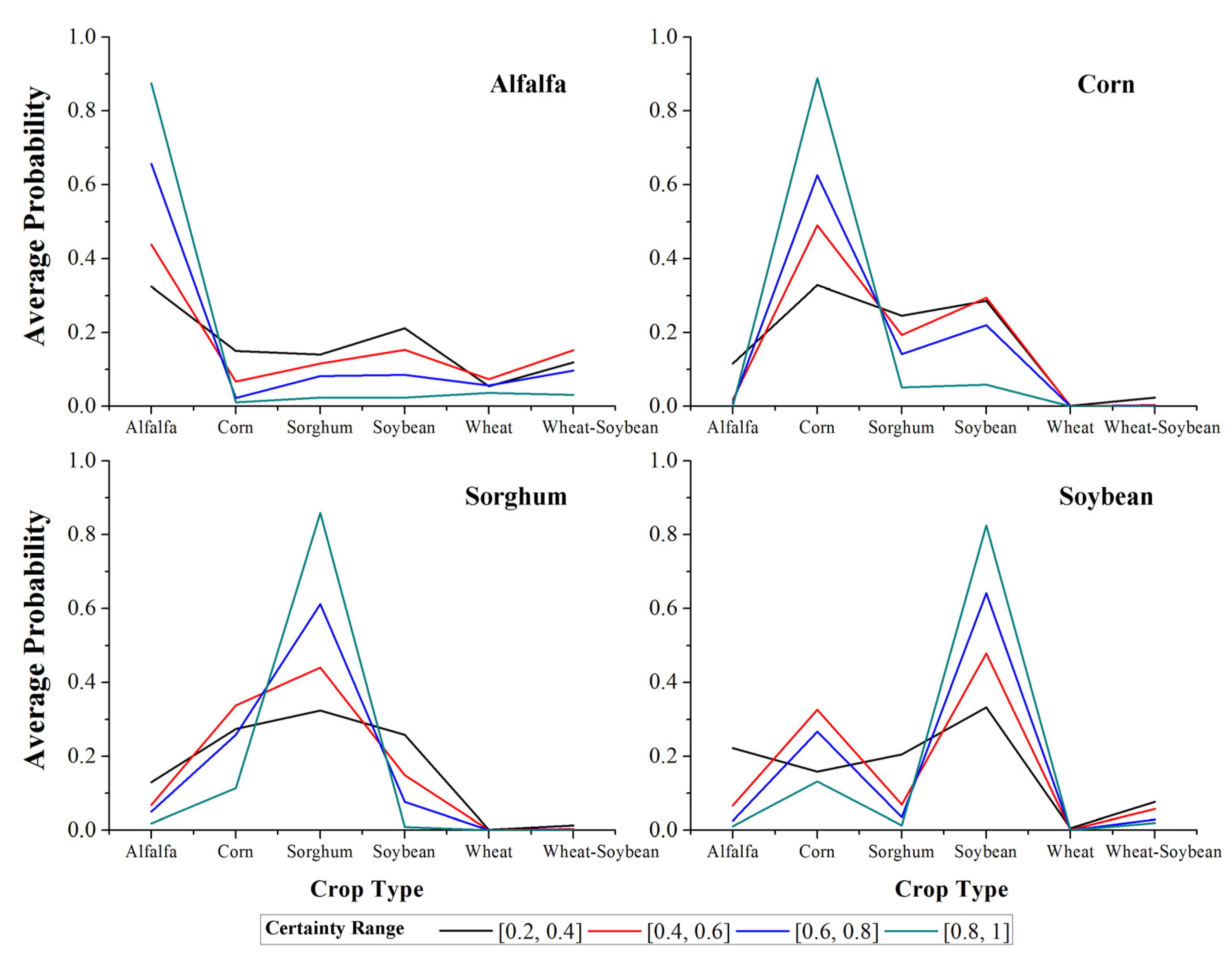
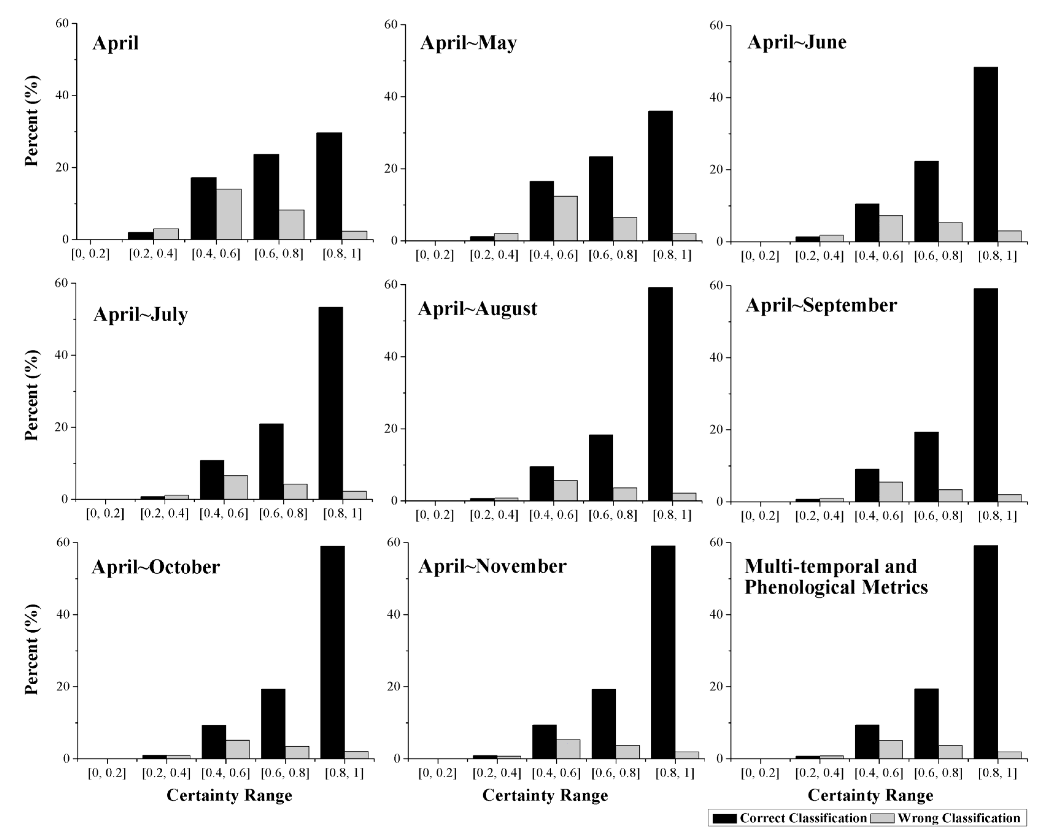
4.4. Classification Certainty

5. Discussion

6. Conclusion
- The augmentation of the time series length can improve crop classification because the separability among different crops, the classification accuracy, and the certainty are increased. In addition, the five-month time series (April to August) was the optimal time series for identifying crops in Kansas because longer time series cannot improve the classification performance (accuracy and certainty). The result also indicated that rather than the entire growing season, relatively short time series have the potential to accurately classify crops.
- For each time series used in this research, additional features improved the classification, as measured by higher separability, classification accuracy, and certainty. Additionally, a portion of these features (such as the first 23 features during the April–November time series) was sufficient to classify the crops accurately, and adding more features after this point had no significant positive effect on crop identification.
- Among the features used in this research, NDVI was the most important feature, as shown by the fact that NDVI features comprised the majority of the top ten features during the eight-month time series (April–November). In addition, the water content index (NDWI) and multi-spectral band data also contributed to distinguishing between the crop types. The phenological metrics features had a relatively low importance and were not selected as the most important features. Moreover, several phenological features, such as EOST and EOSN, can only be obtained after harvest and therefore, cannot contribute to early crop identification using short time series.
- The RF algorithm was used in this research to calculate the importance score, classify the crops, and obtain the classification certainty. When the time series was longer than five months, little change was seen among the top ten features. In addition, the classification accuracy and certainty remained stable when additional features were employed. These results indicate that the RF algorithm is a suitable algorithm for selecting features and classifying crops using a large volume of data.
Appendix
| Month | Time Period in This Study | Date Flag | Corresponding Day of Year (DOY) | Date |
|---|---|---|---|---|
| April | 1 | 097 | 097–104 | 7 April–14 April |
| 2 | 105 | 105–112 | 15 April–22 April | |
| 3 | 113 | 113–120 | 23 April–30 April | |
| May | 4 | 121 | 121–128 | 1 May–8 May |
| 5 | 129 | 129–136 | 9 May–16 May | |
| 6 | 137 | 137–144 | 17 May–24 May | |
| 7 | 145 | 145–152 | 25 May–1 June | |
| June | 8 | 153 | 153–160 | 2 June–9 June |
| 9 | 161 | 161–168 | 10 June–17 June | |
| 10 | 169 | 169–176 | 18 June–25 June | |
| 11 | 177 | 177–184 | 26 June–3 July | |
| July | 12 | 185 | 185–192 | 4 July–11 July |
| 13 | 193 | 193–200 | 12 July–19 July | |
| 14 | 201 | 201–208 | 20 July–27 July | |
| 15 | 209 | 209–216 | 28 July–4 August | |
| August | 16 | 217 | 217–224 | 5 August–12 August |
| 17 | 225 | 225–232 | 13 August–20 August | |
| 18 | 233 | 233–240 | 21 August–28 August | |
| 19 | 241 | 241–248 | 29 August–5 September | |
| September | 20 | 249 | 249–256 | 6 September–13 September |
| 21 | 257 | 257–264 | 14 September–21 September | |
| 22 | 265 | 265–272 | 22 September–29 September | |
| October | 23 | 273 | 273–280 | 30 September–7 October |
| 24 | 281 | 281–288 | 8 October–15 October | |
| 25 | 289 | 289–296 | 16 October–23 October | |
| 26 | 297 | 297–304 | 24 October–31 October | |
| November | 27 | 305 | 305–312 | 1 November–8 November |
| 28 | 313 | 313–320 | 9 November–16 November | |
| 29 | 321 | 321–328 | 17 November–24 November | |
| 30 | 329 | 329–337 | 25 November–2 December |
Acknowledgement
Author Contributions
Conflicts of Interest
References
- Vintrou, E.; Ienco, D.; Begue, A.; Teisseire, M. Data mining, a promising tool for large-area cropland mapping. IEEE J. Sel. Top. Appl. Earth Obs. Remote Sens. 2013, 6, 2132–2138. [Google Scholar] [CrossRef]
- Potgieter, A.B.; Lawson, K.; Huete, A.R. Determining crop acreage estimates for specific winter crops using shape attributes from sequential MODIS imagery. Int. J. Appl. Earth Obs. Geoinf. 2013, 23, 254–263. [Google Scholar] [CrossRef]
- Potgieter, A.B.; Apan, A.; Hammer, G.; Dunn, P. Early-season crop area estimates for winter crops in NE Australia using MODIS satellite imagery. ISPRS J. Photogramm. Remote Sens. 2010, 65, 380–387. [Google Scholar] [CrossRef]
- Howard, D.M.; Wylie, B.K. Annual crop type classification of the US Great Plains for 2000 to 2011. Photogramm. Eng. Remote Sens. 2014, 80, 537–549. [Google Scholar] [CrossRef]
- Atzberger, C. Advances in remote sensing of agriculture: Context description, existing operational monitoring systems and major information needs. Remote Sens. 2013, 5, 949–981. [Google Scholar] [CrossRef]
- Zhang, J.H.; Feng, L.L.; Yao, F.M. Improved maize cultivated area estimation over a large scale combining MODIS-EVI time series data and crop phenological information. ISPRS J. Photogramm. Remote Sens. 2014, 94, 102–113. [Google Scholar] [CrossRef]
- Senturk, S.; Sertel, E.; Kaya, S. Vineyards mapping using object based analysis. In Proceedings of 2013 Second International Conference on Agro-Geoinformatics (Agro-Geoinformatics), Fairfax, VA, USA, 12–16 August 2013.
- Amoros-Lopez, J.; Gomez-Chova, L.; Alonso, L.; Guanter, L.; Zurita-Milla, R.; Moreno, J.; Camps-Valls, G. Multitemporal fusion of Landsat/TM and ENVISAT/MERIS for crop monitoring. Int. J. Appl. Earth Obs. Geoinf. 2013, 23, 132–141. [Google Scholar] [CrossRef]
- Kuenzer, C.; Knauer, K. Remote sensing of rice crop areas. Int. J. Remote Sens. 2013, 34, 2101–2139. [Google Scholar] [CrossRef]
- Cable, J.W.; Kovacs, J.M.; Shang, J.L.; Jiao, X.F. Multi-temporal polarimetric Radarsat-2 for land cover monitoring in northeastern Ontario, Canada. Remote Sens. 2014, 6, 2372–2392. [Google Scholar] [CrossRef]
- Wang, D.; Lin, H.; Chen, J.S.; Zhang, Y.Z.; Zeng, Q.W. Application of multi-temporal ENVISAT ASAR data to agricultural area mapping in the Pearl River Delta. Int. J. Remote Sens. 2010, 31, 1555–1572. [Google Scholar] [CrossRef]
- Jia, K.; Wu, B.; Li, Q. Crop classification using HJ satellite multispectral data in the North China Plain. J. Appl. Remote Sens. 2013, 7, 073576. [Google Scholar] [CrossRef]
- Brown, J.C.; Kastens, J.H.; Coutinho, A.C.; Victoria, D.D.; Bishop, C.R. Classifying multiyear agricultural land use data from Mato Grosso using time-series MODIS vegetation index data. Remote Sens. Environ. 2013, 130, 39–50. [Google Scholar] [CrossRef]
- Murakami, T.; Ogawa, S.; Ishitsuka, N.; Kumagai, K.; Saito, G. Crop discrimination with multitemporal SPOT/HRV data in the Saga Plains, Japan. Int. J. Remote Sens. 2001, 22, 1335–1348. [Google Scholar] [CrossRef]
- Van Niel, T.G.; McVicar, T.R. Determining temporal windows for crop discrimination with remote sensing: A case study in south-eastern Australia. Comput. Electron. Agric. 2004, 45, 91–108. [Google Scholar]
- Wardlow, B.D.; Egbert, S.L.; Kastens, J.H. Analysis of time-series MODIS 250 m vegetation index data for crop classification in the US Central Great Plains. Remote Sens. Environ. 2007, 108, 290–310. [Google Scholar] [CrossRef]
- Hao, P.; Wang, L.; Niu, Z.; Aablikim, A.; Huang, N.; Xu, S.; Chen, F. The potential of time series merged from Landsat-5 tm and HJ-1 CCD for crop classification: A case study for Bole and Manas counties in Xinjiang, China. Remote Sens. 2014, 6, 7610–7631. [Google Scholar] [CrossRef]
- Gallego, J.; Craig, M.; Michaelsen, J.; Bossyns, B.; Fritz, S. Best practices for crop area estimation with remote sensing; European Commission Joint Research Centre: Ispra, Italy, 2010. [Google Scholar]
- Zhou, F.Q.; Zhang, A.N.; Townley-Smith, L. A data mining approach for evaluation of optimal time-series of MODIS data for land cover mapping at a regional level. ISPRS J. Photogramm. Remote Sens. 2013, 84, 114–129. [Google Scholar] [CrossRef]
- Zhong, L.H.; Gong, P.; Biging, G.S. Phenology-based crop classification algorithm and its implications on agricultural water use assessments in California’s Central Valley. Photogramm. Eng. Remote Sens. 2012, 78, 799–813. [Google Scholar] [CrossRef]
- Zhong, L.H.; Gong, P.; Biging, G.S. Efficient corn and soybean mapping with temporal extend ability: A multi-year experiment using Landsat imagery. Remote Sens. Environ. 2014, 140, 1–13. [Google Scholar] [CrossRef]
- Wardlow, B.D.; Egbert, S.L. A comparison of MODIS 250-m EVI and NDVI data for crop mapping: A case study for Southwest Kansas. Int. J. Remote Sens. 2010, 31, 805–830. [Google Scholar] [CrossRef]
- Da Silva, C.A.; Frank, T.; Rodrigues, T.C.S. Discrimination of soybean areas through images EVI/MODIS and analysis based on geo-object. Rev. Bras. Eng. Agric. Ambient. 2014, 18, 44–53. [Google Scholar]
- Low, F.; Michel, U.; Dech, S.; Conrad, C. Impact of feature selection on the accuracy and spatial uncertainty of per-field crop classification using support vector machines. ISPRS J. Photogramm. Remote Sens. 2013, 85, 102–119. [Google Scholar] [CrossRef]
- Vieira, M.A.; Formaggio, A.R.; Renno, C.D.; Atzberger, C.; Aguiar, D.A.; Mello, M.P. Object based image analysis and data mining applied to a remotely sensed Landsat time-series to map sugarcane over large areas. Remote Sens. Environ. 2012, 123, 553–562. [Google Scholar] [CrossRef]
- Loosvelt, L.; Peters, J.; Skriver, H.; De Baets, B.; Verhoest, N.E.C. Impact of reducing polarimetric SAR input on the uncertainty of crop classifications based on the random forests algorithm. IEEE Trans. Geosci. Remote Sens. 2012, 50, 4185–4200. [Google Scholar] [CrossRef]
- Congalton, R.G. A review of assessing the accuracy of classifications of remotely sensed data. Remote Sens. Environ. 1991, 37, 35–46. [Google Scholar] [CrossRef]
- Bloch, I. Information combination operators for data fusion: A comparative review with classification. IEEE Trans. Syst. Man Cybern. Part A: Syst. Humans 1996, 26, 52–67. [Google Scholar] [CrossRef]
- Mountrakis, G.; Im, J.; Ogole, C. Support vector machines in remote sensing: A review. ISPRS J. Photogramm. Remote Sens. 2011, 66, 247–259. [Google Scholar] [CrossRef]
- Breiman, L. Random forests. Mach. Learn. 2001, 45, 5–32. [Google Scholar] [CrossRef]
- Cropscape-Cropland Data Layer. Available online: http://nassgeodata.gmu.edu/CropScape/ (accessed on 2 December 2014).
- Wardlow, B.D.; Egbert, S.L. Large-area crop mapping using time-series MODIS 250-m NDVI data: An assessment for the U.S. Central Great Plains. Remote Sens. Environ. 2008, 112, 1096–1116. [Google Scholar] [CrossRef]
- Masialeti, I.; Egbert, S.; Wardlow, B.D. A comparative analysis of phenological curves for major crops in Kansas. Gisci. Remote Sens. 2010, 47, 241–259. [Google Scholar] [CrossRef]
- Kansas crop planting guide. Available online: http://www.ksre.k-state.edu/bookstore/pubs/l818.pdf (accessed on 23 April 2015).
- Land Processes Distributed Active Archive Center. Available online: http://lpdaac.usgs.gov/ (accessed on 23 April 2015).
- Gao, B.C. NDWI—A normalized difference water index for remote sensing of vegetation liquid water from space. Remote Sens. Environ. 1996, 58, 257–266. [Google Scholar] [CrossRef]
- Viña, A.; Tuanmu, M.-N.; Xu, W.; Li, Y.; Qi, J.; Ouyang, Z.; Liu, J. Relationship between floristic similarity and vegetated land surface phenology: Implications for the synoptic monitoring of species diversity at broad geographic regions. Remote Sens. Environ. 2012, 121, 488–496. [Google Scholar] [CrossRef]
- Remote Sensing Phenology. Available online: http://phenology.cr.usgs.gov/ (accessed on 11 December 2014).
- USDA National agricultural statistics service, 2013 Kansas cropland data layer. Available online: http://www.nass.usda.gov/research/Cropland/metadata/metadata_ks13.htm (accessed on 11 December 2014).
- Surface Reflectance 8-Day L3 Global 500m. Available online: https://lpdaac.usgs.gov/products/MODIS_products_table/mod09a1 (accessed on 12 December 2014).
- Rodriguez-Galiano, V.F.; Ghimire, B.; Rogan, J.; Chica-Olmo, M.; Rigol-Sanchez, J.P. An assessment of the effectiveness of a random forest classifier for land-cover classification. ISPRS J. Photogramm. Remote Sens. 2012, 67, 93–104. [Google Scholar] [CrossRef]
- Liaw, A.; Wiener, M. Randomforest: Breiman and Cutler’s Random Forests for Classification and Regression. Available online: http://cran.r-project.org/web/packages/randomForest/index.html (accessed on 15 December 2014).
- Loosvelt, L.; Peters, J.; Skriver, H.; Lievens, H.; Van Coillie, F.M.B.; De Baets, B.; Verhoest, N.E.C. Random forests as a tool for estimating uncertainty at pixel-level in SAR image classification. Int. J. Applied Earth Obs. Geoinf. 2012, 19, 173–184. [Google Scholar] [CrossRef]
- Van Niel, T.G.; McVicar, T.R.; Datt, B. On the relationship between training sample size and data dimensionality: Monte Carlo analysis of broadband multi-temporal classification. Remote Sens. Environ. 2005, 98, 468–480. [Google Scholar]
- Adam, E.; Mutanga, O. Spectral discrimination of papyrus vegetation (Cyperus Papyrus L.) in swamp wetlands using field spectrometry. ISPRS J. Photogramm. Remote Sens. 2009, 64, 612–620. [Google Scholar] [CrossRef]
- Bruzzone, L.; Roli, F.; Serpico, S.B. An extension of the Jeffreys-Matusita distance to multiclass cases for feature selection. IEEE Trans. Geosci. Remote Sens. 1995, 33, 1318–1321. [Google Scholar] [CrossRef]
- Huang, X.; Zhang, L. An SVM ensemble approach combining spectral, structural, and semantic features for the classification of high-resolution remotely sensed imagery. IEEE Trans. Geosci. Remote Sens. 2013, 51, 257–272. [Google Scholar] [CrossRef]
- Pal, M.; Foody, G.M. Feature selection for classification of hyperspectral data by SVM. IEEE Trans. Geosci. Remote Sens. 2010, 48, 2297–2307. [Google Scholar] [CrossRef]
- Wardlow, B.D.; Kastens, J.H.; Egbert, S.L. Using USDA crop progress data for the evaluation of greenup onset date calculated from MODIS 250-meter data. Photogramm. Eng. Remote Sens. 2006, 72, 1225–1234. [Google Scholar] [CrossRef]
© 2015 by the authors; licensee MDPI, Basel, Switzerland. This article is an open access article distributed under the terms and conditions of the Creative Commons Attribution license (http://creativecommons.org/licenses/by/4.0/).
Share and Cite
Hao, P.; Zhan, Y.; Wang, L.; Niu, Z.; Shakir, M. Feature Selection of Time Series MODIS Data for Early Crop Classification Using Random Forest: A Case Study in Kansas, USA. Remote Sens. 2015, 7, 5347-5369. https://doi.org/10.3390/rs70505347
Hao P, Zhan Y, Wang L, Niu Z, Shakir M. Feature Selection of Time Series MODIS Data for Early Crop Classification Using Random Forest: A Case Study in Kansas, USA. Remote Sensing. 2015; 7(5):5347-5369. https://doi.org/10.3390/rs70505347
Chicago/Turabian StyleHao, Pengyu, Yulin Zhan, Li Wang, Zheng Niu, and Muhammad Shakir. 2015. "Feature Selection of Time Series MODIS Data for Early Crop Classification Using Random Forest: A Case Study in Kansas, USA" Remote Sensing 7, no. 5: 5347-5369. https://doi.org/10.3390/rs70505347