Article

Mapping Above-Ground Biomass in a Tropical Forest in Cambodia Using Canopy Textures Derived from Google Earth

1
Forest Ecology and Conservation Group, Department of Plant Sciences, University of Cambridge, Cambridge CB2 3EA, UK
2
École française d’Extrême-Orient, Siem Reap, Cambodia
3
Department of Geography, National University of Singapore, 1 Arts Link, 117570 Singapore
4
APSARA National Authority, Angkor International Research and Documentation Centre, Siem Reap, Cambodia
5
APSARA National Authority, Department of Forestry Management, Cultural Landscape and Environment, Siem Reap, Cambodia
*
Author to whom correspondence should be addressed.
Remote Sens. 2015, 7(5), 5057-5076; https://doi.org/10.3390/rs70505057
Submission received: 17 December 2014 / Revised: 8 April 2015 / Accepted: 13 April 2015 / Published: 23 April 2015

Abstract

:
This study develops a modelling framework for utilizing very high-resolution (VHR) aerial imagery for monitoring stocks of above-ground biomass (AGB) in a tropical forest in Southeast Asia. Three different texture-based methods (grey level co-occurrence metric (GLCM), Gabor wavelets and Fourier-based textural ordination (FOTO)) were used in conjunction with two different machine learning (ML)-based regression techniques (support vector regression (SVR) and random forest (RF) regression). These methods were implemented on both 50-cm resolution Digital Globe data extracted from Google Earth™ (GE) and 8-cm commercially obtained VHR imagery. This study further examines the role of forest biophysical parameters, such as ground-measured canopy cover and vertical canopy height, in explaining AGB distribution. Three models were developed using: (i) horizontal canopy variables (i.e., canopy cover and texture variables) plus vertical canopy height; (ii) horizontal variables only; and (iii) texture variables only. AGB was variable across the site, ranging from 51.02 Mg/ha to 356.34 Mg/ha. GE-based AGB estimates were comparable to those derived from commercial aerial imagery. The findings demonstrate that novel use of this array of texture-based techniques with GE imagery can help promote the wider use of freely available imagery for low-cost, fine-resolution monitoring of forests parameters at the landscape scale.

Graphical Abstract

1. Introduction

Although tropical forests cover only 6% of the Earth’s surface, they are a crucial reservoir of biodiversity, providing a multitude of ecosystem services from the local to the global scale, such as carbon storage and the provision of timber and non-timber forest products to local communities. Forest loss and associated anthropogenic disturbance contribute approximately 6% to 17% of global carbon emissions [1], with a significant proportion of global deforestation concentrated within the tropics. Tropical forest loss has been especially severe in Southeast Asia [2], especially in countries with turbulent political histories that experienced several decades of war (e.g., Cambodia, Laos and Vietnam). Post-war periods in these countries have seen a sharp rise in forest loss and illegal logging. Cambodia, in particular, has experienced some of the highest percentage rates of deforestation globally [3], with rates increasing through time [4], resulting in a loss of 12,600 km2 of forest between 2000 and 2012 [5].
Payments for ecosystem service (PES) instruments, such as Reduced Emissions from Degradation and Deforestation (REDD+), provide mechanisms to incentivise tropical forest conservation and avoid deforestation through payments that protect forest carbon stocks. The implementation of REDD+ strategies requires quantification of the above-ground biomass (AGB) stored in the forests, from which the carbon storage of a given ecosystem can be estimated. Remote sensing data play an important role in landscape-scale AGB estimation and the subsequent evaluation of land use change impacts on AGB stocks [6]. While remotely-sensed imagery allows us to obtain very high-resolution (VHR) data (pixel size <1 m) over inaccessible forest terrain, such as that found in Cambodia, it is usually expensive to procure, both as a vendor and a customer [7]. Recently, Google Earth™ (GE) has offered free public access to VHR Digital Globe imagery. Although GE has a huge repository of high-resolution imagery (including VHR over tropical forests), this has been underutilized in quantitative environmental research until recently [8].
Aerial imagery is a valuable tool for forest monitoring in tropical countries, offering the potential to characterize forest canopy cover, crown size distributions, AGB and other forest structure parameters. Forest loss and tree removal may influence the canopy structure, which, in turn, has a cascading impact on forest structure and AGB [9]. Furthermore, canopy structure and crown size distribution are intimately linked with forest succession and regeneration. Using aerial imagery, these variables can be characterized at the landscape scale [10]. Additionally, horizontal canopy structure, which is known to influence AGB stocks of open-canopied forest systems [11], can also be characterized via these data. Indeed, a criticism of remote sensing for monitoring tropical forest AGB is that variables related to horizontal canopy structure have not been adequately incorporated or accounted for [10].
Horizontal forest structure and AGB can be determined by texture analysis of high-resolution remote sensing data [10,11]. Texture is a qualitative characterization of a given object in terms of its spatial and structural attributes. Statistical texture measures, notably grey level co-occurrence metrics (GLCMs), are widely used in remote sensing studies of tropical forest AGB and structure [11] and have been applied to moderate-resolution remote sensing data to derive landscape-scale AGB models in Indonesia [12] and the Brazilian Amazon [13]. However, Singh et al. [9] indicate that while GLCM textures are strong predictors for AGB values of forests that have undergone varying rounds of logging, they tend to underestimate field-measured AGB values due to data saturation at higher AGB values. A less common canopy texture technique is Fourier-based textural ordination (FOTO). This method uses a combination of Fourier transforms and ordination approaches (such as principal component analysis (PCA)) to quantify canopy structure and AGB heterogeneity and how this influences AGB variations [10]. This method has been used for quantifying AGB stock variability in varied tropical forested ecosystems, such as coastal mangrove forests [14] and natural and plantation forests [10,15]. Wavelet-derived texture methods are also increasingly used to characterize different forest types, particularly their areal delineation. For example, discrete wavelet transforms (DWT) were used to differentiate five tropical forests with similar canopy heights [16]. Gabor wavelets have been used to delineate different temperate forest types in the Swiss Alps [17]. However, wavelet-based texture analysis holds great promise for the quantification of AGB stocks and forest structure variations. In addition to texture-based methods, machine learning-based modelling techniques are increasingly utilized in AGB modelling. ML is a data-centric analysis technique that provides a robust means of modelling forestry data for both classification and predictive analysis-related tasks, such as estimation of AGB values [18,19].

2. Goal and Objectives

This study examined the utility of three-band remote sensing imagery obtained from two different sources—50-cm resolution Digital Globe imagery (extracted from Google Earth™) and 8-cm VHR aerial imagery—in examining variation in AGB stocks. Different texture-based and machine learning (ML) techniques were used to: (i) compare the utility of GLCMs, Fourier and Gabor wavelet-based texture measures for predicting AGB from both 50-cm and 8-cm aerial data; (ii) identify which of the two ML algorithms, random forest (RF) or support vector regression (SVR), produces better AGB estimation models; and (iii) examine whether the inclusion of height-related variables and canopy cover data improves AGB estimates. These results can facilitate the development of a remote sensing-based AGB monitoring framework that utilises a combination of low-cost/free high-resolution aerial imagery, field data and novel modelling techniques.

3. Materials and Methods
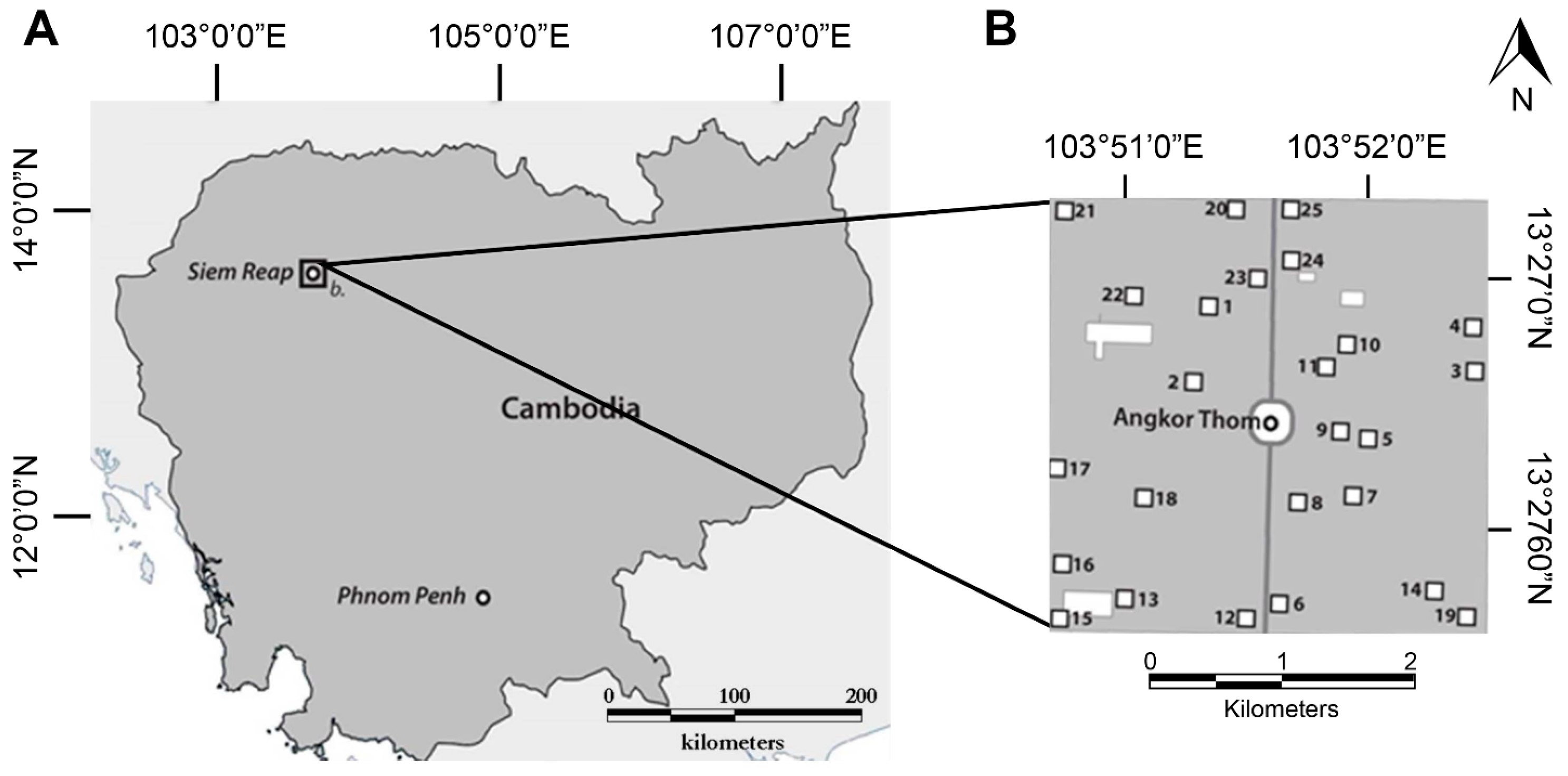
3.1. Study Area

Angkor Thom in northwest Cambodia is a 3 km × 3 km walled city (originally built in the 12th to 13th century AD) located within the Angkor Archaeological Park, much of which is forested (Figure 1).
Figure 1. (A) Regional setting; and (B) Angkor Thom and the location of the 25, 1-ha above-ground biomass (AGB) field plots.
Remotesensing 07 05057 g001
The surrounding forests are semi-evergreen forests dominated by dipterocarp tree species, ranging in height from 25 m to 40 m [20]. While Cambodia has distinct dry and wet seasons (like much of continental SE Asia), these forests are mostly dominated by evergreen tree species. Given its deep cultural significance, historical evolution and current land use changes, Angkor Thom and its associated forests can be considered a “living landscape”. Although these forests enjoy a high level of protection owing to Angkor Thom’s UNESCO World Heritage designation, the issue of tree removal and degradation persists within these forests [21].

3.2. Field Data Collection

Field data collection was conducted from December, 2013, to January, 2014. Twenty five randomly-stratified 1-ha plots were established in the forested portion of Angkor Thom (Figure 1), as per the RAINFOR protocol [22]. One-hectare plots were chosen, as smaller plot sizes may increase the dominance of larger trees, causing an increase in the root-mean-square error (RMSE) [23,24]. Stratification was conducted on the basis of the four forest quadrants that lead to the north, south, east and west gateways of Angkor Thom. All of the forested areas leading inwards have faced different levels of anthropogenic disturbance and have been occupied by different disturbance niches. Plots were randomly located within each of the quadrants. Diameter at breast height (DBH) was recorded for all trees where DBH ≥10 cm. The tree height (H) of 150 trees was measured using a clinometer. A DBH-to-tree height relationship was derived using field-measured tree heights and DBH, which, in turn, was used to estimate the heights of trees for which only DBH was measured. For more detail, see Tables S1–S3. AGB stocks were estimated from tree height and DBH measurements using the following allometric equation recommended by Chave et al. [25]:
A G B = 0.0509 × ρ × D B H 2 × H
Here, ρ represents specific wood density, where a mean value of 0.57 Mg/m3 was used [26]. Aside from the required variables in Equation (1), canopy cover was estimated in each 1-ha plot from 20 to 25 canopy cover readings using a densitometer. More specifically, 20 to 25 canopy cover readings were recorded from random locations within each of the 1-ha plots (Table S2).

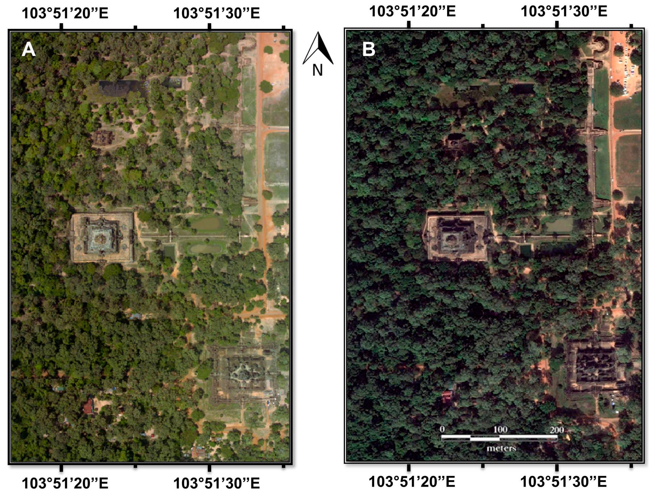
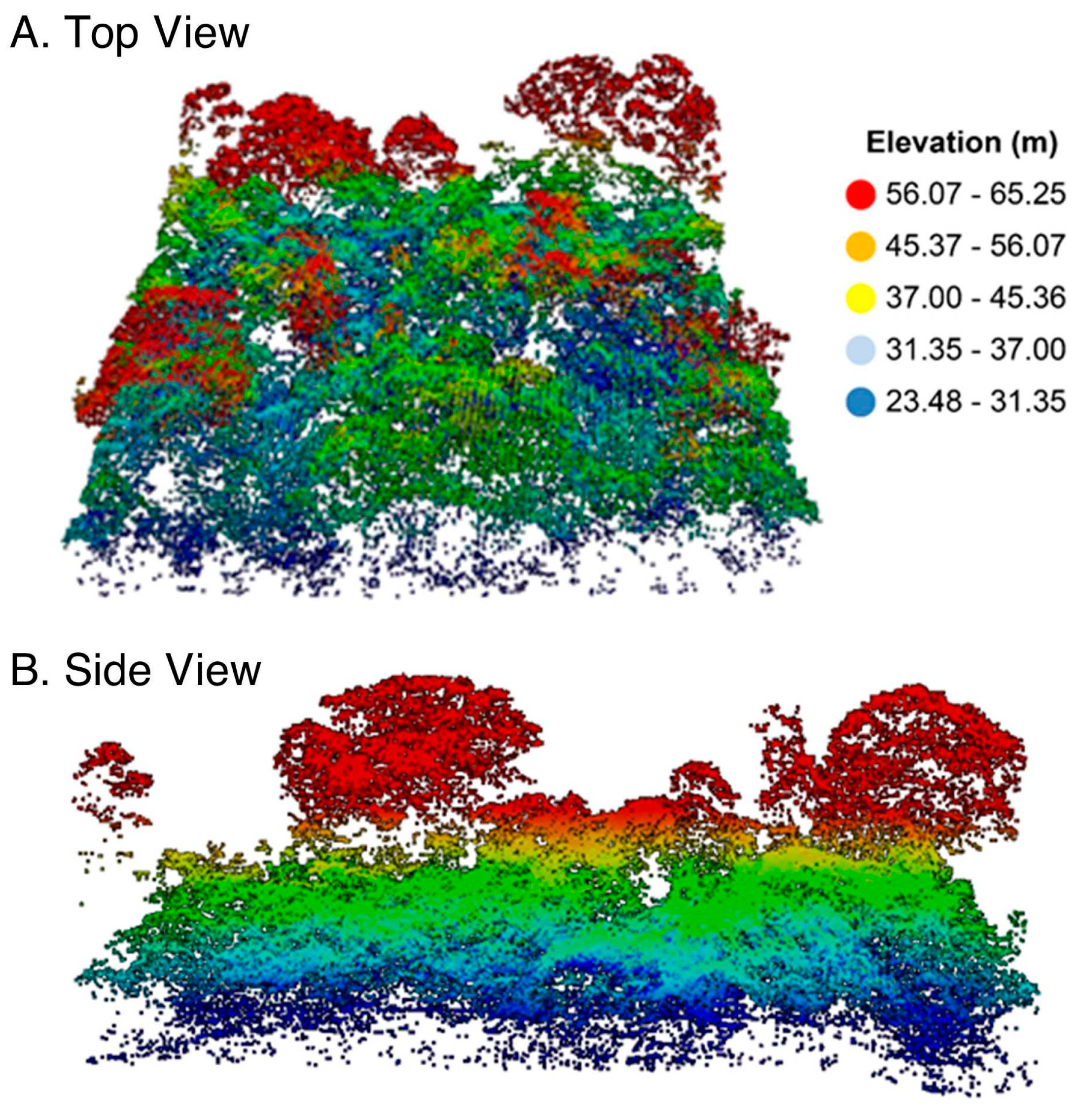
3.3. Analysis of Aerial Imagery Data

Fifty-centimetre resolution Digital Globe data (images dated 26 December 2012) were extracted over Angkor Thom, north-western Cambodia directly from Google Earth™ using Google Satellite Map Downloader® (Version 7.20) [27]. These data have three spectral bands (red, green and blue (RGB)) and covered the entire Angkor Thom area (Figure 1). Eight-centimetre resolution aerial multispectral data were acquired in April 2013, using a 40-megapixel Leica RCD105 medium-format camera, collected by a helicopter at a flying height of 800 m above ground level. Aerial multispectral data also consisted of three RGB spectral bands. The wavelengths of RGB bands for high-resolution aerial data, including those from Google Earth™, are 0.45 to 0.52 nm, 0.52 to 0.60 nm and 9.62 to 0.69 nm, respectively. Radiometric, atmospheric and geometric corrections were conducted by the data provider. Figure 2 shows the 50-cm GE and 8-cm VHR image over a portion of Angkor Thom.
Figure 2. Aerial imagery used in the study: (A) Google Earth™ (GE) imagery and (B) very high-resolution (VHR) imagery (provided by Damian Evans) coverage over a portion of Angkor Thom
Remotesensing 07 05057 g002
Airborne LiDAR data were collected in conjunction with the aerial multispectral RGB data. The LiDAR data consisted of four returns and a point density of 12 points per square metre. Figure 3 shows the LiDAR point cloud-based 3D structure of the forest canopy. The blue regions represent the lowest elevations, while orange to red regions stand for the high tree elevations in the plot.
LiDAR data were used to develop a canopy height model (CHM) as a three-dimensional (3D) representation of the vertical canopy structure. CHMs were generated using FUSION software and are the product of subtracting the digital surface model (DSM) from the assumed digital terrain model (DTM); first and last return, respectively. The LiDAR point cloud-derived products (DTM, DSM and CHM) all had a resolution of 0.5 m. FUSION/LDV is freely available software for processing LiDAR point clouds [28]. In turn, CHM was used for deriving tree heights at the plot scale. See Figure S1 for a detailed workflow.
Figure 3. (A) Top view and (B) Side view of LiDAR point cloud-based 3D structure of forest canopy.
Remotesensing 07 05057 g003

3.4. Texture Analysis of Aerial Imagery

3.4.1. Grey Level Co-Occurrence Matrix

GLCMs quantify the tonal variability of image pixels. There are two main kinds of GLCM texture measures used in the image analyses: (i) first-order or occurrence metrics; and (ii) second-order or co-occurrence metrics. First-order occurrence metrics quantify pixel values at a given location, ignoring the relationship between adjacent pixels (e.g., common statistical measures, such as mean and standard deviation). Second-order co-occurrence metrics account for the relationship between pixels, as well as the probability of pixel occurrence in a given direction. This includes measures, such as entropy and the angular sum of moment [29]. GLCM values were extracted from the three different bands of the VHR and GE aerial imagery using a window size of 3 × 3 in the ENVI image processing software. Details of the GLCM metrics extracted using ENVI can be found in Singh et al. [9].

3.4.2. Fourier-Based Textural Ordination

FOTO aims to identify the gradients of textural variation by coupling two-dimensional (2D) Fourier spectra describing the spatial frequency distribution of image variance in canopy scenes. FOTO algorithms decompose the spatial information contained in an image into its frequency components by applying a 2D fast Fourier transform (FFT), where canopy structure variability can be encompassed within a few spatial frequencies [30]. The spectral and spatial information in the image is decomposed into the frequency domain characterized by F(p, q), which travel in the X and Y directions. This, in turn, is used to obtain Fourier coefficients. In order to best represent the extracted features/associated greyscale variance, a power spectrum was computed by squaring the amplitude of the FFT transform. Averaging was carried out across all orientations to obtain the r-spectrum, which contains the mean values of each frequency [16]. The r-value quantifies the number of times that a pattern is repeated, which, in turn, represents the spatial structure of the canopy within a given window using a select few spatial frequencies obtained by the 2D FFT [10]. The r-spectrum also captures the coarseness gradient-related textural properties, which, in turn, may be related to underlying forest structure properties. Principal component analysis (PCA) was applied to the r-spectrum. The first three principal axes were taken to be the texture indices, which, subsequently, can be used to correlate the stand parameters and biomass dynamics of the different land-use types [14]. In our study, the first PC axis explained around 98% of the variance, while the second PC axis explained 1.2% of the variance. The third PC axis explained 0.2% of the variance. The PC axis beyond this did not explain any variance and, hence, was excluded. The various steps involved in this algorithm are detailed in the flowchart shown in Figure S2.

3.4.3. Gabor Wavelet-Based Texture Measures

Unlike FOTO-based methods, wavelet-based methods belong to the family of spatial frequency-based analysis. Spatial frequency decomposition breaks down imagery data into multiple scales and orientations. The variations in scale and orientation of a given image help capture the textural variation of its pixels, as provided in Equation (2):
ψ θ , v ( z ) = k θ , v 2 σ 2 exp ( k θ , v 2 z 2 2 σ 2 ) [ exp ( i k θ , v ) exp ( σ 2 2 ) ]
where σ = 2π and θ and ν represent the orientation and scale, respectively, of the Gabor wavelet in a given spatial domain. Gabor wavelet analysis produces both real and imaginary parts. The real part encapsulates the texture variation of the canopy and repetitiveness and was retained for analysis [17].

3.5. Machine Learning to Model AGB

3.5.1. Support Vector Regression

SVR accounts for the nonlinearity, non-normality and complexity of ecological data by using kernel functions to map the original input space into a higher-dimension feature space. In Equation (3), y is the variable whose values we seek to predict, and x represents predictor variables that are mapped into the bespoken higher-dimensional feature space using a nonlinear function ϕ(x). That is,
y = ω · ϕ ( x ) + b
where ω is the weight and b is the bias of the regression function. C is a constant used to account for penalized loss when training errors occur [31], as shown in Equation (4):
C ( y ,   f (   x ,   ω ) ) = {     0   i f   | y f (   x ,   ω ) | ε | y f (   x ,   ω ) |   o t h e r w i s e  
SVR then seeks to minimize the square of the weight function and the sum of the permitted errors, ε. The value of ϕ(x) is not known, and kernel functions are used for mapping the predictor variables into higher dimensions [32]. Radial basis function (RBF) is a kernel function that is commonly used to account for such data and which produces robust results compared to other kernels [33,34]. Linear and polynomial kernels were tested statistically, as per Kuhn et al. [35], using correlation coefficients and RMSE to evaluate model performance. The correlation values between field AGB and predicted AGB obtained from different kernels was comparable; however, the lowest RMSE values were obtained from the RBF kernel; thus, linear and polynomial kernels were not used. The RBF kernel function is used for fitting hyper-planes, which allows increasing the separability of the input variables. The purpose of a basic support vector algorithm is to discover a hyper-plane that maximizes the distance between the input variables. The points from each class closest to the hyper-plane are support vectors. By projecting data into a higher dimension, nonlinear data can be visualized to be functioning as linear data. This facilitates the establishment of mathematical relationships between variables [36].

3.5.2. Random Forests Models

RF models fit multiple decision trees to input data using a random subset of the input variables for each tree constructed. For a dataset with n features, square root of n may be used in each subset. A multitude of trees are constructed, and their average is used to construct a new predictive model [37]. RF offers the advantages of being non-parametric, handling a large number of input variables and skewed data and preventing over-fitting [38]. Both of the above modelling techniques were implemented using the caret package in the R programming language. For biomass modelling purposes, 14 of the 25 plots were randomly used for training/calibration purposes, and the remaining 11 plots were used for testing/validation purposes. Plots were randomly assigned to the training or testing set via the “random” function available in R. Prior to relating texture measures to field AGB, the strongly correlated predictor texture variables were removed using the built-in functionalities provided within the caret package. Including strongly correlated predictor variables in the training model leads to the problem of multi-collinearity and over-fitting. The resulting model has limited generalizability and does not strongly predict the unseen validation data. However, by removing the strongly correlated predictors, we can build a parsimonious model containing a small subset of uncorrelated texture variables, which, in turn, helps build robust predictive models.
Training our initial model development used the 14 training plots with 25 iterations for bootstrap-based resampling (these are built-in within the “train” function used to build a model). The final predicted model was used with the test data (in this case, 11 plots) to generate predictions for the target variable. Two ML algorithms were used for generating predictions of field AGB using vertical canopy height, canopy cover and texture measures derived from different methods. The performance of the three models—(i) included vertical canopy height, horizontal canopy structure and texture variables as predictors; (ii) with canopy cover and texture variables; and (iii) with texture variables only—was compared using two different aerial datasets and ML algorithms.

4. Results

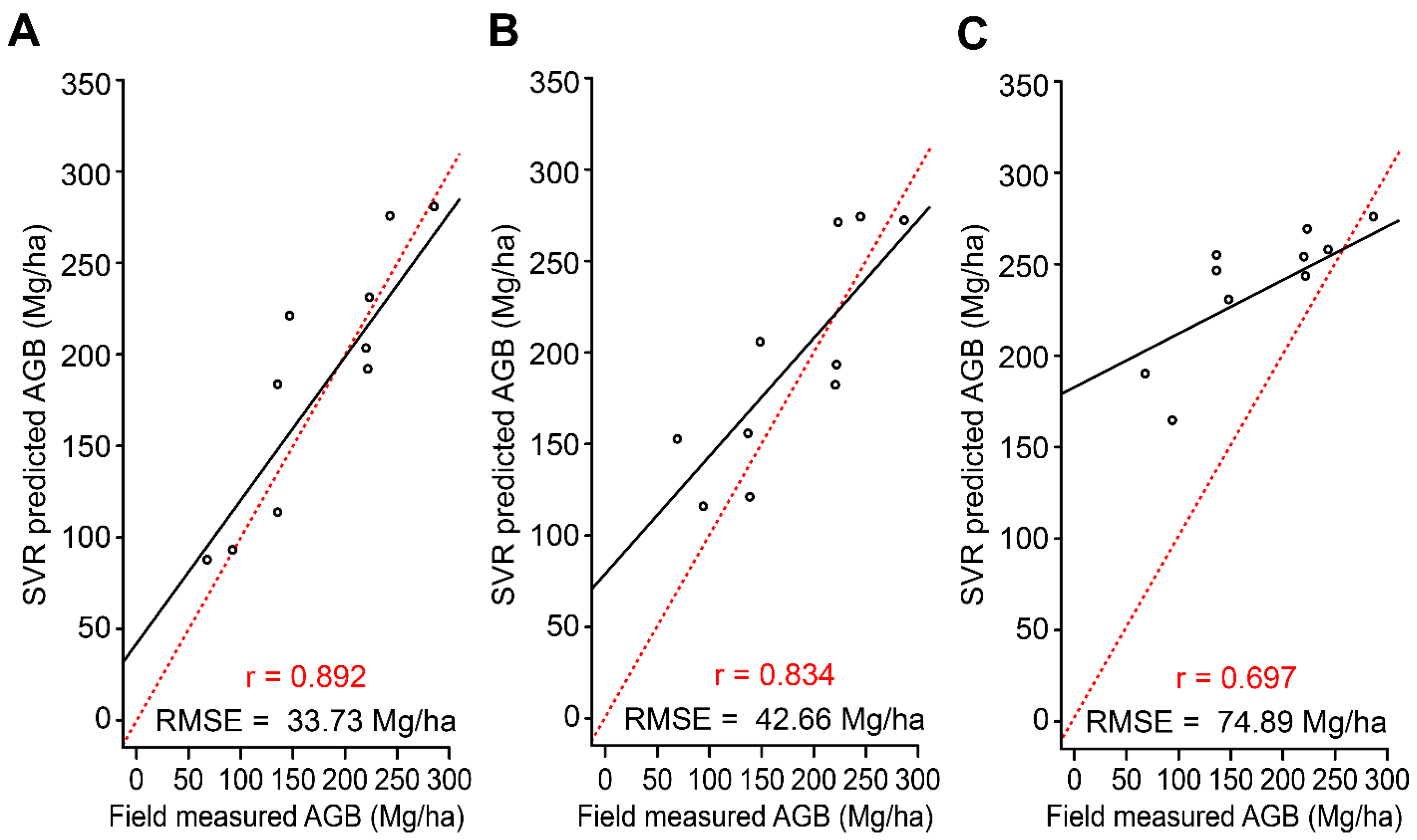
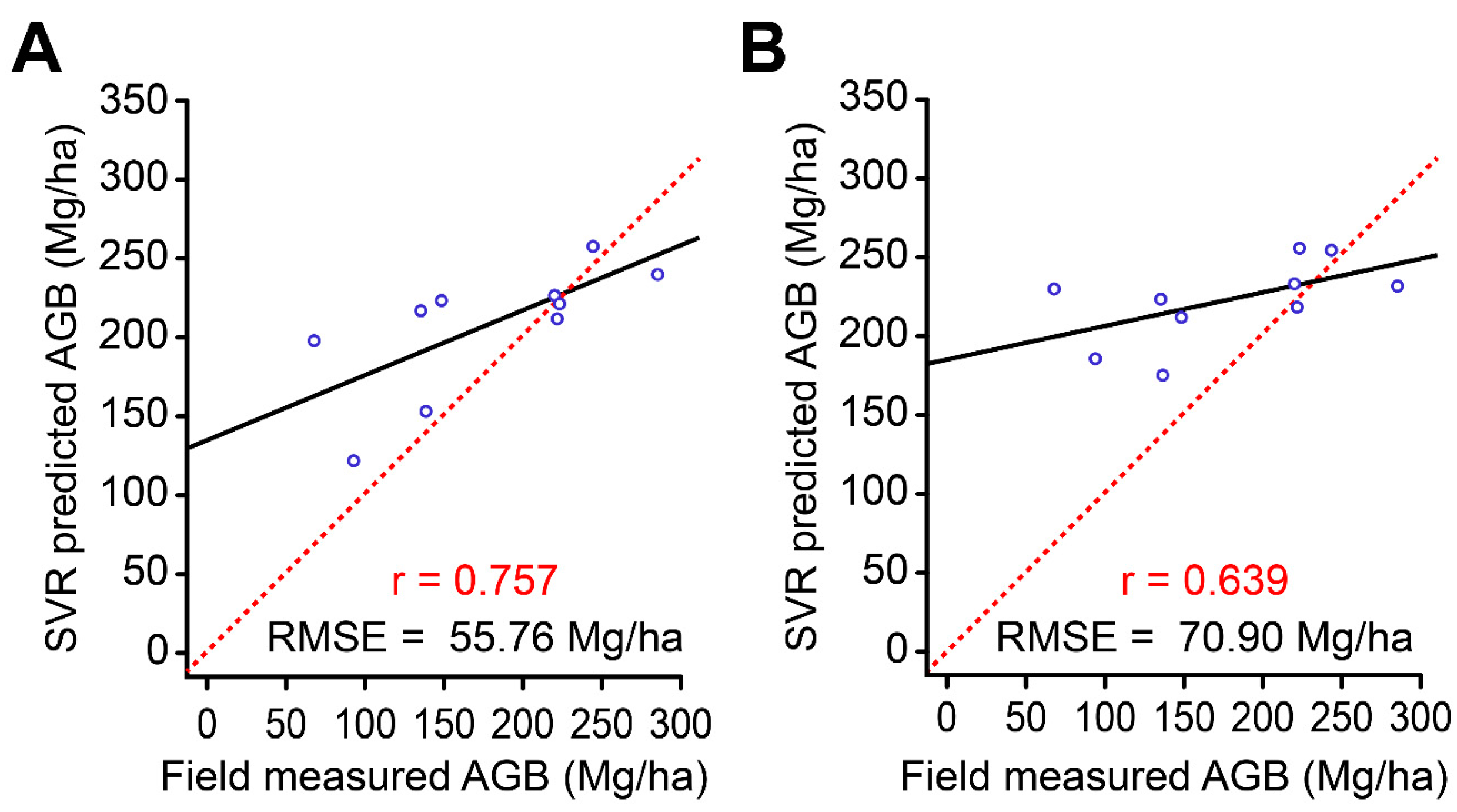
4.1. GLCM-Derived AGB Estimates

The GLCM method achieved strong to very strong positive correlations between SVR-predicted AGB and field-measured AGB for both the 50-cm resolution GE imagery and the 8-cm resolution aerial multispectral imagery, with r-values (Pearson’s product-moment correlation coefficient) ranging from 0.630 to 0.888. Pearson’s correlation was chosen in order to identify any relationship between the field-measured and SVR predicted AGB [39]. As evident in Figure 1 and Figure 2, comparatively high r-values and low RMS errors are obtained from GE imagery compared to those from VHR imagery. For both datasets, the same trend can be observed; correlation coefficient (r) was highest and RMSE was lowest when both horizontal canopy variables (HCV) and vertical canopy height (VCH) were included in the analysis.
AGB estimates from VHR imagery yielded r-values of 0.757 and 0.639 and RMS errors of 55.76 and 70.90 Mg/ha for the first (Figure 4A) and second (Figure 4B) GLCM-derived models, respectively. No significant strength of association was detected for the third GLCM model extracted from GE imagery, which only used texture variables for AGB prediction. Conversely, the AGB estimates from GE imagery yielded: (1) r = 0.892 and RMSE = 33.73 Mg/ha for the first GLCM-derived model, which combined HCV and VCH as predictors (Figure 5A); (2) r = 0.834 and RMSE = 42.66 Mg/ha for the second model, which only accounted for HCV (Figure 5B); and (3) r = 0.697 and RMSE = 74.89 Mg/ha for the third model, which used texture variables (TV) alone (Figure 5C).
Figure 4. Support vector regression (SVR)-predicted AGB vs. field-measured AGB, as derived from VHR imagery via the grey level co-occurrence metric (GLCM) method using (A) horizontal canopy variables (HCV) + vertical canopy height (VCH) and (B) HCV only. Solid black lines represent regression lines; red dashed lines represent 1:1 correspondence lines.
Remotesensing 07 05057 g004
Visual comparison of Figure 4 and Figure 5 revealed that the two GLCM models derived from VHR imagery exhibit more pronounced deviations from their respective 1:1 correspondence lines than did the three GE models. All five GLCM models, however, underestimated AGB at lower field values (AGB < 200 Mg/ha) and overestimation at higher values (AGB > 250 Mg/ha).
Furthermore, when the GLCM method was employed in conjunction with random forest regression (RFR), the resulting RFR-predicted AGB also displayed strong to very strong positive associations with field-measured AGB, although the RFR-based r-values were slightly lower than their SVR counterparts. Specifically, for GE imagery, RF regression yielded: (1) r = 0.793 and RMSE = 54.34 Mg/ha for the first GLCM model, incorporating HCV + VCH; (2) r = 0.786 and RMSE = 60.7 Mg/ha for the HCV-only model; and (3) r = 0.47 and RMSE = 76.07 Mg/ha for the TV-only model. For VHR imagery, the RFR-derived values were r = 0.783 and RMSE = 57.51 Mg/ha for the HCV + VCH model. Except for this last RMSE value, all of the other RFR-based RMS errors are higher than their SVR counterparts.
Figure 5. SVR-predicted AGB vs. field-measured AGB, as derived from Google Earth™ imagery via the GLCM method using (A) HCV + VCH, (B) HCV only and (C) texture variables (TV) only. Solid black lines represent regression lines; red dashed lines represent 1:1 correspondence lines.
Remotesensing 07 05057 g005

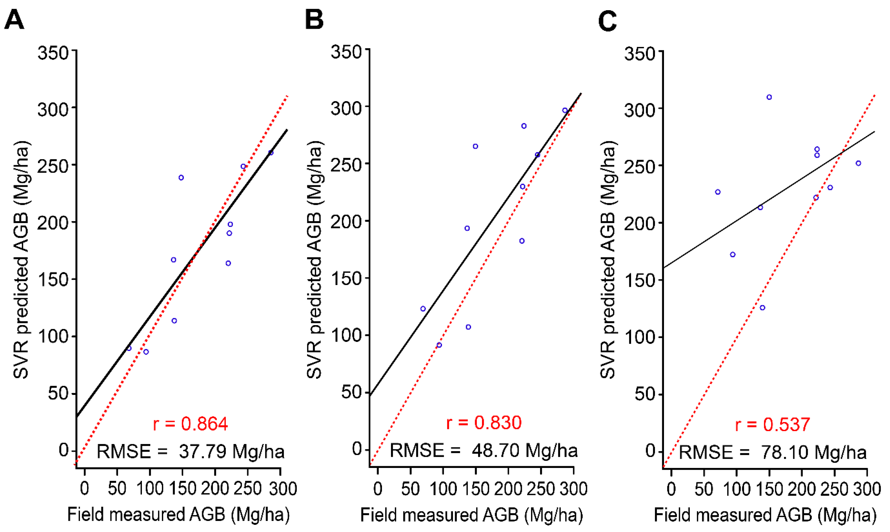
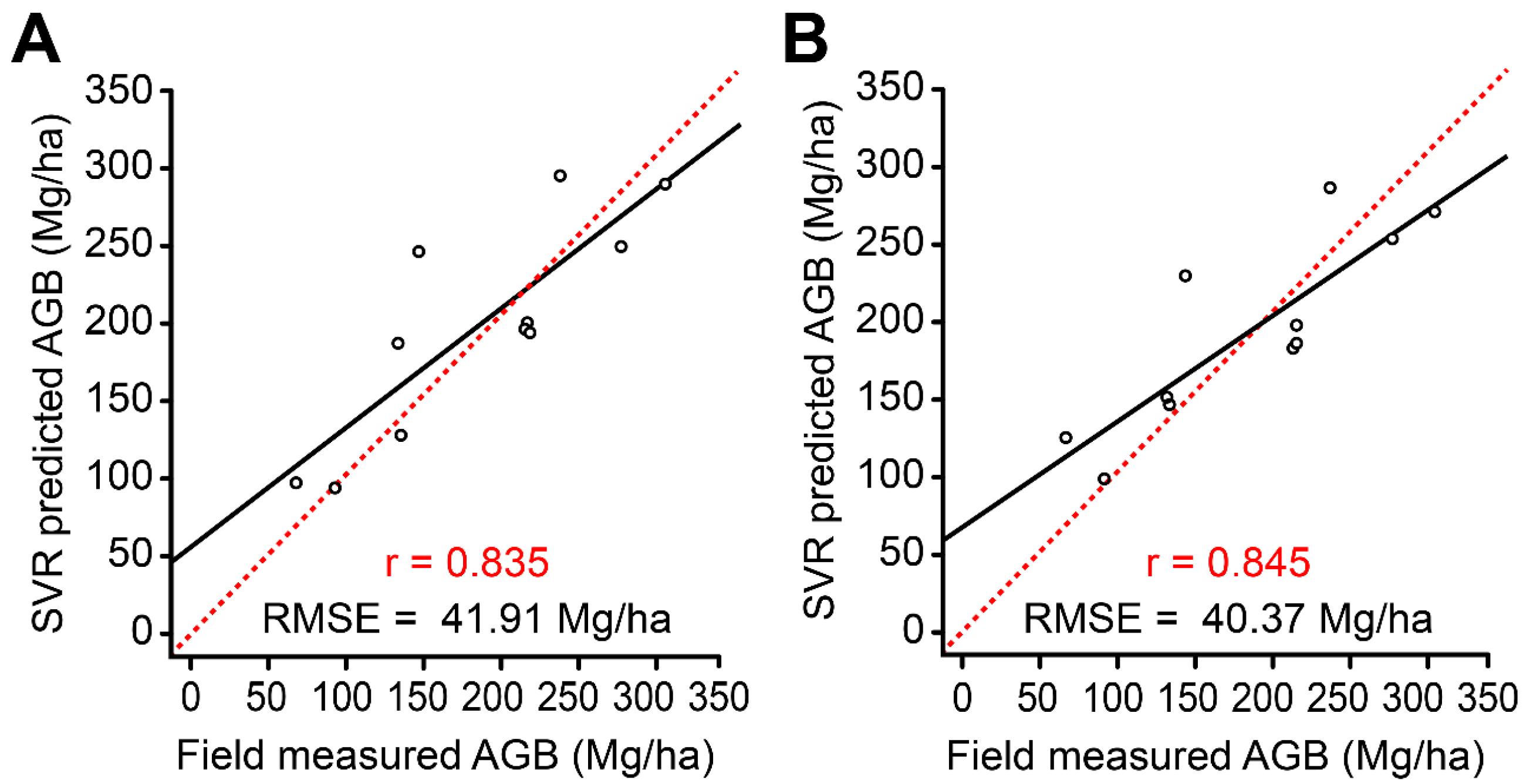
4.2. FOTO-Derived AGB Estimates

The results of the FOTO analyses were comparable to those of the GLCM analyses, establishing strong to very strong positive associations between FOTO-derived AGB estimates and field-measured AGB, e.g., with SVR-based r-values of 0.537 to 0.864 and corresponding RFR-based r-values of 0.695 to 0.864.
Trends in both r and RMSE values were similar to those of the GLCM-derived models (Figure 6), where: (1) the HCV + VCH model had the highest r and lowest RMSE, followed by (2) the HCV-only model and (3) the TV-only model with the lowest and highest RMSE. These trends were observed for both SVR-based and RFR-based values: the r-values of Models (1), (2) and (3) for the SVR-based AGB estimates were 0.864, 0.830 and 0.537, respectively, with corresponding RMS errors of 37.79, 48.70 and 78.10 Mg/ha. For the RFR-based AGB estimates, the respective r-values of Models (1), (2), and (3) were 0.745, 0.695 and 0.503, with corresponding RMS errors of 55.63, 64.25 and 76.63 Mg/ha.
For the SVR-predicted AGB, from GE imagery via the FOTO method, the first model (HCV and VCH as predictors) yielded r = 0.835 and RMSE = 41.91 Mg/ha (Figure 7A), while the second model (HCV alone) yielded r = 0.845 and RMSE = 40.37 Mg/ha (Figure 7B). For analogous analyses using RFR, the corresponding results were: (1) r = 0.764 and RMSE = 51.063 Mg/ha for the HCV + VCH model; and (2) r = 0.864 and RMSE = 48.89 Mg/ha for the HCV-only model.
In the case of FOTO-derived AGB estimates from GE imagery, the second model (which excludes the vertical canopy height) exhibited the strongest positive association between SVR-predicted AGB and field-measured AGB, as well as between RFR-derived AGB and field-measured AGB. For FOTO models extracted from VHR imagery, no significant association was detected for the third model, which only used texture variables for AGB prediction.
Figure 6. SVR-predicted AGB vs. field-measured AGB, as derived from VHR imagery via the Fourier-based textural ordination (FOTO) method using (A) HCV + VCH, (B) HCV only and (C) TV only. Solid black lines represent regression lines; red dashed lines represent 1:1 correspondence lines.
Remotesensing 07 05057 g006
Figure 7. SVR-predicted AGB vs. field-measured AGB, as derived from Google Earth™ imagery via the FOTO method using (A) HCV and VCH, and (B) TV only. Solid black lines represent regression lines; red dashed lines represent 1:1 correspondence lines.
Remotesensing 07 05057 g007

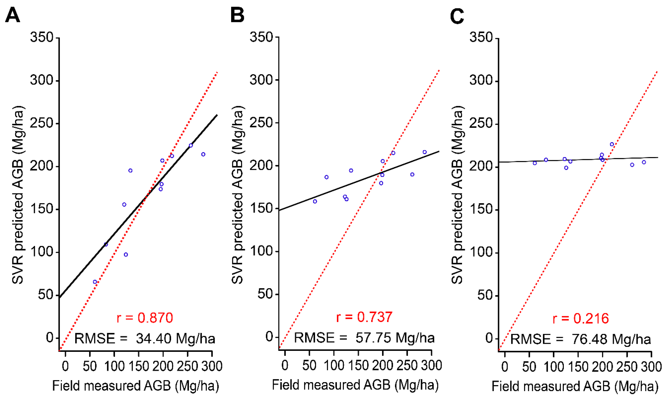
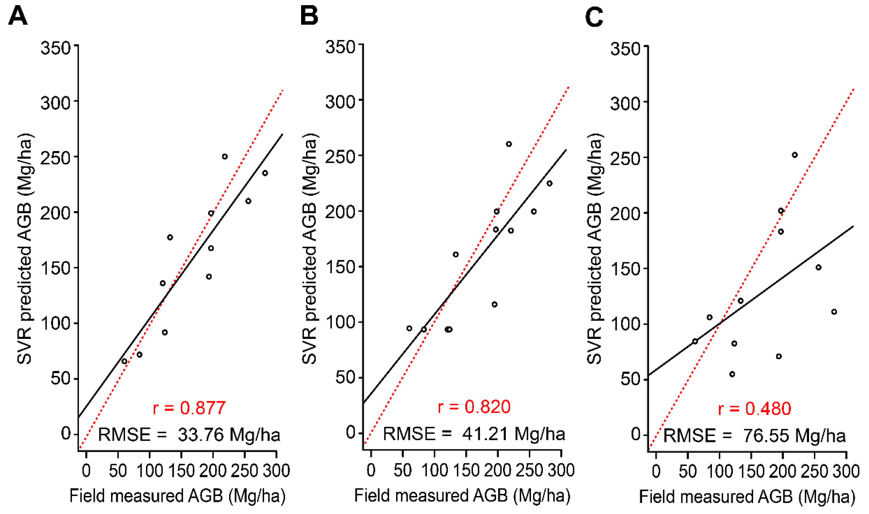
4.3. Gabor Wavelet-Derived AGB Estimates
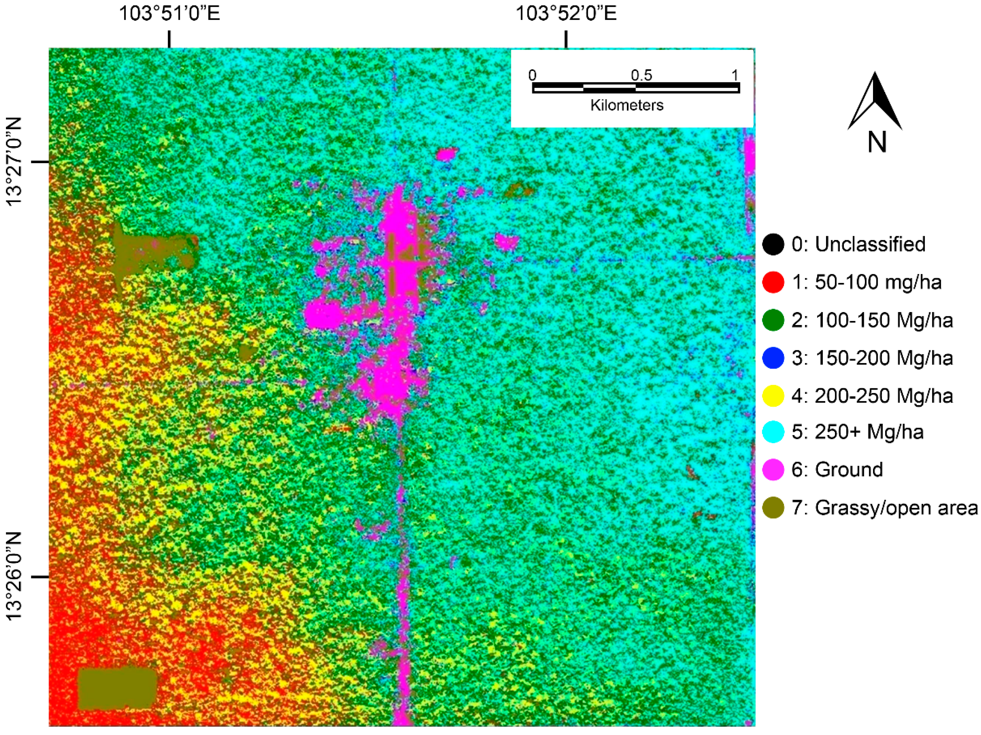
Figure 8 presents three scatter plots corresponding to three Gabor wavelet-derived models obtained from VHR imagery using different combinations of forest biophysical parameters. The following trends in both r and RMSE values are similar to those of the GLCM- and FOTO-derived models: (1) the HCV + VCH model has the highest r and lowest RMSE, followed by (2) the HCV-only model and (3) the TV-only model with the lowest r and highest RMSE. More specifically, the r-values of Models (1), (2) and (3) for the SVR-based AGB estimates are 0.870, 0.737 and 0.216, respectively, with corresponding RMS errors of 34.40, 57.75 and 76.48 Mg/ha, respectively.
Figure 8. SVR-predicted AGB vs. field-measured AGB, as derived from VHR imagery via the Gabor method using (A) HCV + VCH, (B) HCV only and (C) TV only. Solid black lines represent regression lines; red dashed lines represent 1:1 correspondence lines.
Remotesensing 07 05057 g008
Figure 9 presents three scatter plots corresponding to three Gabor wavelet-derived models obtained from GE imagery using different combinations of forest biophysical parameters. The trends in both r and RMSE values were similar to that of the GLCM- and FOTO-derived models (0.877, 0.820 and 0.480, with corresponding RMS errors of 33.76, 41.21 and 76.55 Mg/ha, respectively).
Figure 9. SVR-predicted AGB vs. field-measured AGB, as derived from Google Earth™ imagery via the Gabor method using (A) HCV + VCH, and (B) HCV only and (C) TV only. Solid black lines represent regression lines; red dashed lines represent 1:1 correspondence lines.
Remotesensing 07 05057 g009

4.4. Mapping AGB

Field-measured AGB values for Cambodia showed considerable variation (range: 44.55 to 323 Mg/ha, mean 181.1 ± 16.6 Mg/ha). This study developed different GLCM-derived and FOTO-derived models in conjunction with SVR and RFR, many of which capture AGB variations to a high level of accuracy. Table 1 summarizes the various method and model combinations and their corresponding r and RMSE values for both Google Earth™ and commercial VHR imagery.
Table 1. Summary of the different method and model combinations used in AGB prediction. RF, random forest.
Model Combination50 cm Google Earth8 cm Aerial Multispectral
RMSE (Mg/ha)Association with Field AGB (r)RMSE (Mg/ha)Association with Field AGB (r)
GLCM
HCV + VCHSVR33.730.89255.760.757
(RF)(54.34)(0.793)(57.8)(0.787)
HCV onlySVR42.660.83470.900.639
(RF)(60.78)(0.78)n/an/a
TV onlySVR74.890.697n/an/a
(RF)(76.07)(0.47)n/an/a
FOTO
HCV + VCHSVR41.910.83537.790.864
(RF)(53.2)(0.758)(56.039)(0.732)
HCV onlySVR40.370.84548.700.830
(RF)(44.23)(0.86)(57.32)(0.72)
TV onlySVRn/an/a78.100.537
(RF)n/an/a(74.061)(0.52)
Gabor
HCV + VCHSVR33.760.8734.400.870
(RF)46.80.74254.30.808
HCV onlySVR41.210.82057.750.737
(RF)60.180.625n/a0.68
TV onlySVR76.550.48076.480.216
(RF)61.10.54n/a0.17
Of all the remote sensing models presented in this study, the AGB estimates derived via a combination of vertical canopy structure, ground canopy cover variables and GLCM texture variables within an SVR modelling framework showed the strongest association with field-measured AGB (r = 0.892). Figure 10 shows the resulting spatial distribution of AGB in Angkor Thom, as derived using all of the aforementioned parameters.
AGB exhibits a distinct pattern across Angkor Thom, with the highest values recorded at the northeast corner and the lowest in the southwest corner (Figure 3).
Figure 10. Spatial distribution of above-ground biomass in Angkor Thom, based on a best-fit SVR + vertical canopy + horizontal canopy + GLCM model.
Remotesensing 07 05057 g010

5. Discussion

5.1. Spatial Patterns of AGB in Angkor Thom

AGB stocks differed across the Angkor Thom landscape, with some areas holding high AGB stocks (up to 300 Mg/ha), while other areas held much lower stocks. A distinct pattern of AGB stock distribution can be seen across the site, with the southern portion (especially the southwest) having a much lower AGB stock value. Since the southern portion of Angkor Thom serves as the main access to most of the historical buildings in the area, it receives a significant flow of tourists. This massive inflow of people is likely to cause anthropogenic disturbance, thereby influencing AGB in the area. However, as one moves toward the archaeological sites, there is an increased level of security (restricted tourist access, presence of security guards), dramatically reducing the chances of illegal forest loss.
The variation in AGB distribution may be seen as a problem of “leakage” that is usually associated with protected areas. A similar situation has been observed in the buffer zones around tropical protected areas [31]. Closer proximity to the core of the protected area affords a much higher level of protection as compared to buffer zones; core areas are thus subject to lower rates of forest loss and resource extraction. Another major cause of AGB loss that is apparent not only in Angkor Thom, but also in other parts of tropical Asia [32] is the proximity of an area to various sources of anthropogenic disturbance, such as roads.

5.2. The Effectiveness of Different Model Combinations for Estimating AGB

5.2.1. The Importance of Structural Parameters

The present study employed several model combinations to estimate AGB stocks and their spatial distribution. Previous studies have utilized solely multispectral sources to estimate AGB [10,15], although in the majority of the texture models—GLCM, FOTO and Gabor wavelets—the inclusion of vertical height data provided marginally improves AGB estimates. However, ground-measured canopy cover percentage was strongly associated with field AGB values (r = 0.698). Previous studies in the tropics using different datasets, and modelling approaches have established the role of vertical canopy height in producing accurate estimates of AGB [23]. However, the corresponding role of the percentage of canopy cover was not previously examined in the literature. While this study establishes the role of canopy cover in explaining AGB variation, there are no universally accepted protocols for measuring canopy cover, either in the field or using remote sensing data. This makes the comparison of our canopy cover-based results with other research difficult.

5.2.2. Performance of Different Modelling Approaches

In all cases, the SVR-based models outperformed the RFR-based models. SVR also produced more robust estimates of AGB variation than did multiple regression models [40]. ML methods, such as SVR, are capable of producing robust and generalizable models of forest parameters. Furthermore, they can characterize forest structural complexity at finer scales, which is poorly captured by traditional linear and non-linear regression models. This enables detailed AGB models that can facilitate monitoring and conservation activities. In addition to the efficacy of ML models, it was found that GE aerial imagery (in conjunction with different texture measures) can produce robust AGB estimates.

5.2.3. Performance of Google Earth™ Imagery vs. VHR Imagery for AGB Estimation

GLCM-, Gabor- and Fourier-based texture variables derived from GE and VHR imagery (along with vertical canopy height and canopy cover) showed a strong association with field-measured AGB. In all cases, SVR-predicted AGB values were more similar to field AGB with lower RMSE than were RF-predicted AGB values. SVR is known to produce accurate AGB estimates [40] and to outperform other ML techniques, such as RF regression [41]. On the basis of the results obtained using both ML techniques, textural variables, both statistical and Fourier-based, are powerful predictors of AGB stock variation. The strength of association did not decline considerably between models that used both horizontal and vertical variables and those that used horizontal variables (canopy cover and texture metrics) only. Thus, in open-canopied forest ecosystems, such as the one in our study area, consideration of vertical canopy structure does not significantly improve AGB estimates, while inclusion of percentage canopy cover estimates is more important. However, models that used a combination of percentage canopy cover and texture variables (derived from either of the methods) tended to underestimate AGB values, especially for lower AGB values, whereas the inclusion of vertical canopy height improved the fit between predicted AGB and the 1:1 line. Texture variables themselves had limited utility for AGB prediction. AGB predicted using GLCM variables derived from GE imagery, VHR-based Fourier texture and Gabor wavelet variables had a moderate strength of association with field AGB values and deviated considerably from the 1:1 line.
Ground canopy cover is often ignored in most tropical forest inventories, whereas this study makes a strong case for its inclusion in AGB monitoring. Vertical canopy height is an important variable in its own right, but its collection either through LiDAR surveys or field measurements can be expensive and/or cumbersome.

5.3. Implications of Freely Available Remote Sensing Imagery for Conservation

This study has shown the utility of freely available remote sensing sources, such as GE and other Digital Globes, for robust, quantitative mapping of forest parameters, such as AGB, although this is rarely conducted. However, see Ploton et al. [42] for an example of AGB estimation using GE for forests in the Western Ghats, India. Such data sources could allow regular and cost-effective monitoring of tropical forested ecosystems.
While high-resolution GE imagery is not available for the entire Asian tropics (especially some inaccessible forested areas), its coverage is increasing. Other endeavours, such as the Digital Globe Foundation, offer free/low-cost VHR imagery for researchers. Structural parameters, such as canopy height, improve the accuracy of AGB estimations, but are relatively difficult and expensive to obtain. Thus, multispectral-only models derived from VHR Digital Globe imagery could play an important role in the repeated monitoring of tropical landscape-scale AGB stocks. Repeated monitoring is vital for accurate reporting, monitoring and verification of forest carbon stocks for conservation instruments, such as REDD+, to support enforcement and enable reliable accounting of ecosystem service provision [43], especially at sites and in ecosystems that are dynamic and affected by surrounding land use decisions and external stressors [44]. However, there is a need to test these models in other ecosystems (notably, closed-canopy forests, mangroves) at different spatial scales, different plot sizes and with other VHR data to improve their general applicability. Finally, not much is known about the data quality of the different image sources present within the GE database, acquisition errors and pre-processing algorithms applied to them. Detailed information relating to acquisition conditions and pre-processing protocols are needed for aerial data (including GE acquired data) to improve the interpretability of results.

6. Conclusions

This study highlights the potential to harness the power of freely-available Digital Globe imagery, such as Google Earth™, in conjunction with novel methods, such as grey level co-occurrence metrics, Gabor wavelets and Fourier-based textural ordination, to quantify biophysical forest parameters of importance to conservation. This study was unique in the range of texture methods utilized, in addition to the comparison of freely available and commercial imagery. Combinations of these techniques were able to quantify fine-scale changes and gradients in forest parameters, such as AGB across a disturbed, open canopy site that is experiencing several threats to forest permanence.
The testing and comparison of GE-derived results against traditional remotely-sensed data sources highlights its potential utility as part of a framework for robust, low-cost, fine-resolution, quantitative mapping of forest parameters, such as above-ground biomass, at the landscape scale in open-canopied forests. The use of freely available data sources, such as GE, could allow regular and cost-effective monitoring of imperilled tropical forested ecosystems in the future. Future studies should focus on the use of the presented framework for repeated monitoring, comparing the different modelling methods to see which best represent changes in forest parameters through time.

Acknowledgments

We are grateful to the APSARA National Authority for permission to undertake field research in the Angkor Thom area, including Bun Chamrouen and Ley Kimsy for their assistance in the field. So Malay, Martin Polkinghorne, Son Rothaphum and the Robert Christie Foundation made essential contributions to the logistical and administrative aspects of the field programme. We thank PT McElhanney Indonesia for their contribution to the LiDAR acquisition and acknowledge support and funding from the eight institutions of the Khmer Archaeology LiDAR Consortium: the APSARA Authority, the University of Sydney, the École française d’Extrême Orient, Société Concessionaire d’Aéroport, the Hungarian Southeast Asian Research Institute, Japan-APSARA Safeguarding Angkor, the Archaeology and Development Foundation and the World Monuments Fund.

Author Contributions

Minerva Singh developed the research concept, collected the field data and performed data analysis. Damian Evans provided the commercial airborne aerial data and LiDAR data and performed the pre-processing operations on these. Daniel A. Friess helped develop the methodology and interpret the data analysis results. Both Damian Evans and Daniel A. Friess advised on the research direction. Boun Suy Tan and Chan Samean Nin provided logistical support and arranged permits, research assistants and access to the study area. Minerva Singh wrote the manuscript with contributions and approval from all of the authors.

Supplementary Files

Supplementary File 1

Conflicts of Interest

The authors declare no conflict of interest.

References

  1. Pan, Y.; Birdsey, R.; Fang, J.; Houghton, R.; Kauppi, P.; Kurz, W.; Phillips, O. A large and persistent carbon sink in the world’s forests. Science 2011, 333, 988–993. [Google Scholar] [CrossRef] [PubMed]
  2. Sodhi, N.; Koh, L.; Brook, B.; Ng, P. Southeast Asian biodiversity: An impending disaster. Trends Ecol. Evol. 2004, 19, 654–660. [Google Scholar] [CrossRef] [PubMed]
  3. Hansen, M.; Potapov, P.; Moore, R.; Hancher, M.; Turubanova, S.; Tyukavina, A.; Thau, D.; Stehman, S.; Goetz, S.; Loveland, T.; et al. High-resolution global maps of 21st-century forest cover change. Science 2013, 342, 850–853. [Google Scholar] [CrossRef] [PubMed]
  4. Southworth, J.; Nagendra, H.; Cassidy, L. Forest transition pathways in Asia—Studies from Nepal, India, Thailand and Cambodia. J. Land Use Sci. 2012, 7, 51–65. [Google Scholar] [CrossRef]
  5. Zsombor, P. Loss of Forest in Cambodia among Worst in the World. The Cambodia Daily, 19 November 2013. [Google Scholar]
  6. Jakubowski, M.; Li, W.; Guo, Q.; Kelly, M. Delineating individual trees from LiDAR data: A comparison of vector-and raster-based segmentation approaches. Remote Sens. 2013, 5, 4163–4186. [Google Scholar] [CrossRef]
  7. Mumby, P.; Green, E.; Edwards, A.; Clark, C. The cost-effectiveness of remote sensing for tropical coastal resources assessment and management. J. Environ. Manag. 1999, 55, 157–166. [Google Scholar] [CrossRef]
  8. Friess, D.; Kudavidanage, E.; Webb, E. The digital globe is our oyster. Front. Ecol. Environ. 2011, 9, 542–552. [Google Scholar] [CrossRef]
  9. Singh, M.; Malhi, Y.; Bhagwat, S. Evaluating land use and aboveground biomass dynamics in an oil palm-dominated landscape in Borneo using optical remote sensing. J. Appl. Remote Sens. 2014, 8, 83695–83695. [Google Scholar] [CrossRef]
  10. Bastin, J.; Barbier, N.; Couteron, P.; Adams, B.; Shapiro, A.; Bogaert, J.; de Cannière, C. Aboveground biomass mapping of African forest mosaics using canopy texture analysis: Towards a regional approach. Ecol. Appl. 2014, 24, 1984–2001. [Google Scholar] [CrossRef]
  11. Drake, J.; Knox, R.; Dubayah, R.; Clark, D.; Condit, R.; Blair, J.; Hofton, M. Above-ground biomass estimation in closed canopy neotropical forests using LiDAR remote sensing: Factors affecting the generality of relationships. Glob. Ecol. Biogeogr. 2003, 12, 147–159. [Google Scholar] [CrossRef]
  12. Wijaya, A.; Kusnadi, S.; Gloaguen, R.; Heilmeier, H. Improved strategy for estimating stem volume and forest biomass using moderate resolution remote sensing data and GIS. J. For. Res. 2010, 21, 1–12. [Google Scholar] [CrossRef]
  13. Lu, D. The potential and challenges of remote sensing based biomass estimates. Int. J. Remote Sens. 2006, 27, 1297–1328. [Google Scholar] [CrossRef]
  14. Singh, M.; Malhi, Y.; Bhagwat, S. Biomass estimation of mixed forest landscape using a Fourier transform texture-based approach on very-high-resolution optical satellite imagery. Int. J. Remote Sens. 2014, 35, 3331–3349. [Google Scholar] [CrossRef]
  15. Proisy, C.; Couteron, P.; Fromard, F. Predicting and mapping mangrove biomass from canopy grain analysis using Fourier-based textural ordination of IKONOS images. Remote Sens. Environ. 2007, 109, 379–392. [Google Scholar] [CrossRef]
  16. Kennel, P.; Tramon, M.; Barbier, N.; Vincent, G. Canopy height model characteristics derived from airborne laser scanning and its effectiveness in discriminating various tropical moist forest types. Int. J. Remote Sens. 2013, 34, 8917–8935. [Google Scholar] [CrossRef]
  17. Wang, Z.; Boesch, R.; Ginzler, C. Forest delineation of aerial images with Gabor wavelets. Int. J. Remote Sens. 2012, 33, 2196–2213. [Google Scholar] [CrossRef]
  18. Goetz, S.; Baccini, A.; Laporte, N.; Johns, T.; Walker, W.; Kellndorfer, J.; Houghton, R.; Sun, M. Mapping and monitoring carbon stocks with satellite observations: A comparison of methods. Carbon Balance Manag. 2009, 4, 2–8. [Google Scholar] [CrossRef] [PubMed]
  19. Zhang, J.; Huang, S.; Hogg, E.; Lieffers, V.; Qin, Y.; He, F. Estimating spatial variation in Alberta forest biomass from a combination of forest inventory and remote sensing data. Biogeosciences 2014, 11, 2793–2808. [Google Scholar] [CrossRef] [Green Version]
  20. Maxwell, J. Vegetation and vascular flora of the Ban Saneh Pawng area, Lai Wo subdistrict, Sangklaburi district, Kanchanaburi Province, Thailand. Nat. Hist. Bull. Siam Soc. 1995, 43, 131–170. [Google Scholar]
  21. Wales, N. Combining Remote Sensing Change Detection and Qualitative Data to Examine Landscape Change in the Context of World Heritage. Ph.D. Thesis, University of Sydney, Sydney, Australia, October 2012. [Google Scholar]
  22. Marthews, T.; Metcalfe, D.; Malhi, Y.; Phillips, O.; Huasco, W.; Riutta, T.; Jaén, M.; Girardin, C.; Urrutia, R.; Butt, N. Measuring Tropical Forest Carbon Allocation and Cycling: A RAINFOR-GEM Field Manual for Intensive Census Plots (v2.2); University of Oxford: Oxford, UK, 2012. [Google Scholar]
  23. Asner, G.; Mascaro, J. Mapping tropical forest carbon: Calibrating plot estimates to a simple LiDAR metric. Remote Sens. Environ. 2014, 140, 614–624. [Google Scholar] [CrossRef]
  24. Meyer, V.; Saatchi, S.; Chave, J.; Dalling, J.; Bohlman, S.; Fricker, G.; Robinson, C.; Neumann, M.; Hubbell, S. Detecting tropical forest biomass dynamics from repeated airborne LiDAR measurements. Biogeosciences 2013, 10, 1957–1992. [Google Scholar] [CrossRef]
  25. Chave, J.; Andalo, C.; Brown, S.; Cairns, M.; Chambers, J.; Eamus, D.; Folster, H.; Fromard, F.; Higuchi, N.; Kira, T.; et al. Tree allometry and improved estimation of carbon stocks and balance in tropical forests. Oecologia 2005, 145, 87–99. [Google Scholar] [CrossRef] [PubMed]
  26. Brown, S.; Iverson, L.; Prasad, A.; Liu, D. Geographical distributions of carbon in biomass and soils of tropical Asian forests. Geocarto Int. 1993, 8, 45–59. [Google Scholar] [CrossRef]
  27. Google Satellite Maps Downloader. Available online: http://www.allallsoft.com/gsmd/ (accessed on (20 December 2012).
  28. McGaughey, R. Fusion/ldv: Software for LiDAR Data Analysis and Visualization [Computer Program]; U.S. Department of Agriculture, Forest Service, Pacific Northwest Research Station: Seattle, WA, USA, 2010. [Google Scholar]
  29. St-Louis, V.; Pidgeon, A.; Radeloff, V.; Hawbaker, T.; Clayton, M. High-resolution image texture as a predictor of bird species richness. Remote Sens. Environ. 2006, 105, 299–312. [Google Scholar] [CrossRef]
  30. Couteron, P.; Pélissier, R.; Nicolini, E.; Paget, D. Predicting tropical forest stand structure parameters from Fourier transform of very high-resolution remotely sensed canopy images. J. Appl. Ecol. 2005, 42, 1121–1128. [Google Scholar] [CrossRef] [Green Version]
  31. Yu, P.; Chen, S.; Chang, I. Support vector regression for real-time flood stage forecasting. J. Hydrol. 2006, 328, 704–716. [Google Scholar] [CrossRef]
  32. Yu, X.; Wang, X.; Chen, J. Support vector machine regression for reactivity parameters of vinyl monomers. J. Chil. Chem. Soc. 2011, 56, 746–751. [Google Scholar] [CrossRef]
  33. Paneque-Gálvez, J.; Mas, J.-F.; More, G.; Cristobal, J.; Orta-Martinez, M.; Luz, A.C.; Gueze, M.; Macia, M.J.; Reyes-Garcia, V. Enhanced land use/cover classification of heterogeneous tropical landscapes using support vector machines and textural homogeneity. Int. J. Appl. Earth Obs. Geoinf. 2013, 23, 372–383. [Google Scholar] [CrossRef]
  34. Zeng, Z.; Hsieh, W.W.; Shabbar, A.; Burrows, W.R. Seasonal prediction of winter extreme precipitation over Canada by support vector regression. Hydrol. Earth Syst. Sci. 2011, 15, 65–74. [Google Scholar] [CrossRef]
  35. Kuhn, M. Caret: Classification and Regression Training, R package version 4.58 2014; Available online: http://CRAN.R-project.org/package=caret (accessed on 21 April 2015).
  36. Lantz, B. Machine Learning with R; Packt Publishing Ltd.: Birmingham, UK, 2013. [Google Scholar]
  37. Breiman, L. Random forests. Mach. Learn. 2001, 45, 5–32. [Google Scholar] [CrossRef]
  38. Mascaro, J.; Detto, M.; Asner, G.; Muller-Landau, H. Evaluating uncertainty in mapping forest carbon with airborne LiDAR. Remote Sens. Environ. 2011, 115, 3770–3774. [Google Scholar] [CrossRef]
  39. Townend, J. Practical Statistics for Environmental and Biological Scientists; John Wiley & Sons: Hoboken, NJ, USA, 2013. [Google Scholar]
  40. Chen, G.; Hay, G.; St-Onge, B. A GEOBIA framework to estimate forest parameters from LiDAR transects, QuickBird imagery and machine learning: A case study in Quebec, Canada. Int. J. Appl. Earth Obs. Geoinf. 2012, 15, 28–37. [Google Scholar] [CrossRef]
  41. Shataee, J. Forest attributes estimation using aerial laser scanner and TM data. For. Syst. 2013, 22, 484–496. [Google Scholar]
  42. Ploton, P.; Pélissier, R.; Proisy, C.; Flavenot, T.; Barbier, N.; Rai, S.N.; Couteron, P. Assessing aboveground tropical forest biomass using Google Earth canopy images. Ecol. Appl. 2012, 22, 993–1003. [Google Scholar] [CrossRef] [PubMed]
  43. Gupta, A.; Lövbrand, E.; Turnhout, E.; Vijge, M. In pursuit of carbon accountability: The politics of REDD+ measuring, reporting and verification systems. Curr. Opin. Environ. Sustain. 2012, 4, 726–731. [Google Scholar] [CrossRef]
  44. Friess, D.; Phelps, J.; Garmendia, E.; Gómez-Baggethun, E. Payments for ecosystem services (PES) in the face of external biophysical stressors. Glob. Environ. Chang. 2015, 30, 31–42. [Google Scholar] [CrossRef]

