1. Introduction
Land surface temperature (LST) is a very important parameter in the surface process of land-air interaction [
1,
2]. Due to their very high spatial resolution, the thermal band data of the Landsat series, such as the Landsat 5 Thematic Mapper (TM) and the Landsat 7 Enhanced Thematic Mapper (ETM), have been widely applied for LST retrieval for such studies as surface energy budget estimation [
3,
4], surface moisture and evapotranspiration monitoring [
5,
6], urban heat island monitoring [
7,
8] and environmental biogeochemistry process simulation [
9], requiring LST as a basic input.
The Landsat 8 thermal infrared (TIR) instrument designed with two TIR bands is very suitable for the split-window algorithm for LST retrieval. Recently, Rozenstein
et al. [
10] adapted the two-factor split-window algorithm of Qin
et al. [
11] for Landsat 8 Thermal Infrared Sensor (TIRS) data. Jiménez-Muñoz
et al. [
12] also adapted their single-channel (SC) algorithms and split-window algorithms to Landsat 8 TIRS data for LST retrieval. However, several artifacts, including banding and absolute calibration discrepancies that violate the requirements in some scenes [
13], had been observed in the TIRS data. Recently, the United States Geological Survey (USGS) issued a notice on its websites relating to the calibration of Landsat 8 TIRS thermal bands [
14]. Prior to the early-2014 update, users might subtract 0.29 W/(m
2·sr·μm) from every TIRS Band 10 calibrated radiance value and 0.51 W/(m
2·sr·μm) for every TIRS Band 11 calibrated radiance value to provide values closer (on average) to the actual radiances. The root mean square (RMS) variability in the required adjustment was roughly 0.12 W/(m
2·sr·μm) (0.8 K) for Band 10 and 0.2 W/(m
2·sr·μm) (1.75 K) for Band 11 [
15]. Moreover, the USGS pointed out that, given the larger uncertainty in the Band 11 values, users should work with TIRS Band 10 data as a single spectral band (like Landsat 7 Enhanced Thematic Mapper Plus (ETM+)) and should not attempt a split-window correction using both TIRS Bands 10 and 11. Therefore, it is still necessary to develop a practical algorithm with detailed determination of the required parameters for LST retrieval from the single Landsat 8 TIRS Band 10 data.
Several LST retrieval algorithms had been developed for previous Landsat series (such as TM and ETM+) with single TIRS band data. The widely used mono-window algorithm developed by Qin
et al. [
16] requires three essential parameters for LST retrieval from the one TIR band data of Landsat TM/ETM+: ground emissivity, atmospheric transmittance and effective mean atmospheric temperature. The method to determine the atmospheric transmittance was given in Qin
et al. [
16] through simulation of atmospheric conditions with the LOWTRAN 7 program. A practicable approach to estimating the effective mean atmospheric temperature from local meteorological observation was also proposed in the paper, when the
in situ atmospheric profile data are unavailable at the satellite pass, which is the general case in the real world, especially for the images in the past. However, one of the main limitations in this algorithm is that the range of water vapor content was designed from 0 to 3 g·cm
−2, which limits LST retrieval beyond these values [
17]. The SC algorithm developed by Jiménez-Muñoz and Sobrino [
18] is a water vapor- and emissivity-dependent method to minimize the required input data for LST retrieval from the Landsat 5 TM data [
18]. Since input data were minimized to only one atmospheric parameter, an error in water vapor content estimation could increase the error in LST retrievability of the SC algorithm. The possible errors in LST retrieval of the SC algorithm are also expected to be increased with the amount of atmospheric water vapor content. The SC algorithm had been updated and extended to Landsat 4 and Landsat 7 band data in Jiménez-Muñoz
et al. [
19], in which the feasibility had been analyzed through look-up tables (LUTs) to avoid the problem relevant to uncertainties introduced from fitting the atmospheric parameters to water vapor content for their estimation.
Both the mono-window algorithm and single-channel algorithm require atmospheric profiles to model the radiative transfer process. The atmosphere has important effects on the remote sensing of LST [
20,
21,
22]. The required parameters for atmospheric thermal radiance can be calculated from atmospheric profiles obtained from local temporarily coincident radiosondes [
16]. Masiello
et al. [
23] presented an atmospheric profile forecasting method for the required parameters with the Spinning Enhanced Visible and Infrared Imager (SEVIRI) data and Infrared Atmospheric Sounding Interferometer (IASI) data [
23]. The SEVIRI is on-board the geostationary meteorological satellites covering Europe, Africa and part of South America. For the regions where the
in situ atmospheric profile data were unavailable at Landsat 8 satellite overpass, the local station measurements of climatological data have to be used for estimation of the atmospheric effects [
16].
The objective of this paper is to develop an improved mono-window (IMW) algorithm for LST retrieval from the Landsat 8 TIRS data, considering the USGS’s notice on calibration of the data. In the following sections, we firstly present the derivation of the algorithm and the computation of the brightness temperature for the LST retrieval. Then, we establish the approaches to estimate the required parameters (i.e., effective mean atmospheric temperature, atmospheric transmittance and ground emissivity) for the algorithm. Thirdly, we perform the sensitivity analysis of the algorithm for the parameters and validate it by the simulated data for various situations of seven typical atmospheres. Finally, we present an example of applying the algorithm to Nanjing and its vicinity in east China for LST retrieval.
2. Development of the IMW Algorithm for Landsat 8 Data
The theoretical basis of thermal remote sensing is that the observed thermal radiance by the remote sensor is mainly from the ground emittance, which, according to the blackbody theorem of radiance, can be determined as a function of temperature at a specific wavelength,
i.e., the thermal range of the spectrum [
20,
21,
24]. However, the atmosphere through which the ground emittance travels to reach the sensor in space has significant effects on the observed thermal radiance. At the same time, the ground is not a perfect blackbody for thermal emittance [
25]. This makes the retrieval of land surface temperature from the observed thermal radiance in space become much more complicated, because the effects from both the atmosphere and the ground have to be considered for the LST retrieval in order to obtain an accurate result. Generally, the LST retrieval from the thermal band data of a remote sensing system can be done through the solution of the thermal radiance transfer equation expressing the composition of the observed thermal radiance by the system in space.
The thermal radiance reaching Landsat 8 TIRS can be divided into three parts: the ground emittance, which is attenuated by atmospheric absorption when traveling through the atmosphere to reach the TIRS sensor, the upwelling atmospheric emittance representing the thermal capability of the atmosphere and the downwelling atmospheric emittance reflected by the ground as a non-blackbody and travelling through the atmosphere to reach the sensor. Considering all of these possible effects from both the atmosphere and the ground, according to Qin
et al. [
16] and Sobrino
et al. [
20], the observed thermal radiance for Landsat 8 TIRS can be expressed as follows for remote sensing of LST:
where
Ts is land surface temperature in Kelvin degrees;
Ti is the brightness temperature of Landsat 8 TIRS band
i; τ
i and ε
i are the atmospheric transmittance and ground emissivity, respectively, for band
i;
Bi(
Ti) represents the observed thermal radiance by the Landsat 8 TIRS, which is expressed as the Planck function at brightness temperature
Ti for band
i;
Bi(
Ts) represents the ground emittance expressed as the Planck function at surface temperature
Ts for band
i;
Ii↓ and
Ii↑ are the downwelling atmospheric emittance and upwelling atmospheric emittance, respectively, for band
i.
Provided that the ground emissivity and atmospheric transmittance can be estimated and assuming the land surface as Lambertian, Qin
et al. [
16] had developed a mono-window algorithm through the solution of Equation (1) for LST retrieval from Landsat 5 TM data, which only have one thermal band (Band 6). Derivation of the algorithm was composed of several reasonable assumptions and approximations used to solve
Ts from Equation (1). The upwelling and downwelling atmospheric emittances were computed as an integrative function of atmospheric emittance (expressed as the Planck radiance function with profile air temperature) at various altitudes and approximated through a mean atmospheric emittance with an effective mean atmospheric temperature (
Ta). Moreover, Planck’s radiance function was linearized through Taylor expansion to approximate the radiance of the ground by the received radiance. With these assumptions and approximations, the LST was solved from Equation (1) for Band 6 (
i = 6) data of Landsat 5 TM as follows:
where
Ts is the LST in Kelvin degrees;
Ta is the effective mean atmospheric temperature;
T6 is the brightness temperature of Landsat 5 TM Band 6;
a6 and
b6 are the coefficients used to approximate the derivative of the Planck radiance function for the thermal band; and
C6 and
D6 are the internal parameters for the algorithm based on the atmospheric parameters and ground emissivity.
Though Landsat 8 TIRS has two thermal bands (10 and 11), only data from Band 10 are suitable at the moment for LST retrieva1 due to the larger uncertainty in the Band 11 values [
13,
14,
15]. Therefore, we improved the mono-window algorithm in the following form for LST retrieval from the Landsat 8 TIRS Band 10 data:
where
Ts is the LST retrieved from the Landsat 8 TIRS Band 10 data;
Ta is the effective mean atmospheric temperature;
T10 is the brightness temperature of Landsat 8 TIRS Band 10;
a10 and
b10 are the constants used to approximate the derivative of the Planck radiance function for the TIRS Band 10 given in
Table 1;
C10 and
D10 are the internal parameters for the algorithm, given as follows:
where τ
10 is atmospheric transmittance of Landsat 8 TIRS Band 10 and ε
10 is the ground emissivity for the band. The improvement was mainly in the determination of the three required parameters (τ
10, ε
10 and
Ta) in the mono-window algorithm for LST retrieval from Landsat 8 TIRS Band 10 data, presented in the following sections. Thus, our algorithm can be termed an improved mono-window (IMW) algorithm for LST retrieval from the available Landsat 8 TIRS Band 10 data.
Table 1.
Determination of coefficients a10 and b10 for the Landsat 8 TIRS Band 10.
Table 1.
Determination of coefficients a10 and b10 for the Landsat 8 TIRS Band 10.
| Temperature Range | a10 | b10 | R2 |
|---|
| 20 °C–70 °C | −70.1775 | 0.4581 | 0.9997 |
| 0 °C–50 °C | −62.7182 | 0.4339 | 0.9996 |
| −20 °C–30 °C | −55.4276 | 0.4086 | 0.9996 |
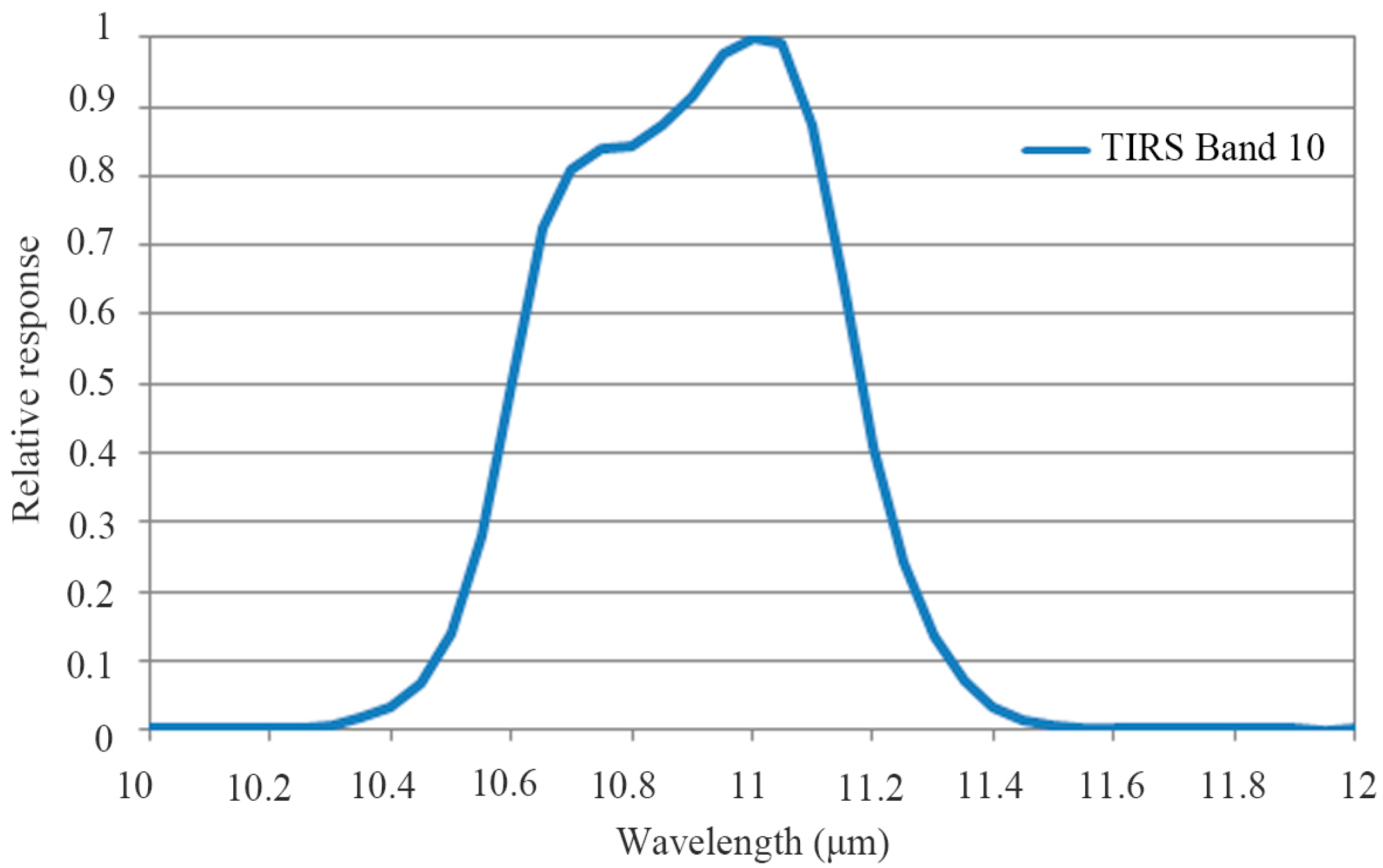
Meanwhile, the TIRS Band 10 (10.6–11.2 µm) of Landsat 8 is different with TM Band 6 (10.4–2.5 µm) of Landsat 5. The upwelling radiance, the downwelling atmospheric radiance and atmospheric transmittance should all be reprocessed according to the spectral region of TIRS Band 10 and its spectral response function:
where
X10 is a weighted average value of radiance or transmittance in TIRS Band 10,
X(
λ) is any spectral parameter considered as radiance and transmittance and
f(
λ) is the spectral response function given in
Figure 1.
Figure 1.
Spectral response function of Landsat 8 TIRS Band 10.
Figure 1.
Spectral response function of Landsat 8 TIRS Band 10.
3. Computation of Brightness Temperature
Retrieval of LST from Landsat 8 TIRS data is with the premise that brightness temperature Ti can be computed for the pixels of Band 10 by the mono-window algorithm (Equation (3)). Since the observed thermal radiance for Band 10 of Landsat 8 TIRS is transformed into digital numbers (DNs) for storage and transfer in a format of 16 digits, which gives the range of 0–65,535, we are able to compute the brightness temperature from Landsat 8 TIRS data through transformation of the DN value into thermal radiance and then conversion of the radiance into brightness temperature.
Considering the calibration notices of USGS [
14], the DN value of Landsat 8 TIRS band data can be converted into thermal spectral radiance through the radiance rescaling factors provided in the metadata file of Landsat 8 data as follows:
where
Ri is the spectral radiance (W·m
−2·sr
−1·μm
−1) of band
i;
Mi is the band-specific multiplicative rescaling factor for band
i;
Ai is the band-specific additive rescaling factor for band
i; and
Qi is the DN value for the quantized and calibrated standard product pixel of band
i;
Oi is the offsets issued by USGS for the calibration of TIRS bands. The values of factors
Mi and
Ai can be obtained from the metadata file of Landsat 8 image. However, according to USGS [
14], the offset
O10 of the images before February 3, 2014, is 0.29 (W·m
−2·sr
−1·μm
−1) for TIRS Band 10, and
O10 of the images after February 3, 2014, should not be considered, because the USGS has reprocessed the data including that radiance offsets. For convenience, we present the values in
Table 2.
The thermal spectral radiance
R computed from Equation (7) for Band 10 can be converted to brightness temperature through approximation of the Planck radiance function using the thermal constants provided in the metadata file:
where
T10 is the brightness temperature (K) of Band 10;
K1 and
K2 are the band-specific thermal conversion constants for Band 10.
Table 2 shows the values of constants
K1, and
K2, which can also be found in the metadata file of the Landsat 8 image.
Table 2.
Constants for computing brightness temperature from Landsat 8 TIRS Band 10 data.
Table 2.
Constants for computing brightness temperature from Landsat 8 TIRS Band 10 data.
| M10 | A10 | O10 (W·m−2·sr−1·μm−1) | K1 (W·m−2·sr−1·μm−1) | K2 (K) |
|---|
| 0.0003342 | 0.1 | 0.29 | 774.89 | 1321.08 |
4. Determination of Effective Mean Atmospheric Temperature
The upwelling atmospheric radiance is usually estimated by the effective mean atmospheric temperature (
Ta) [
20]. The determination of
Ta requires the distribution of atmospheric temperature and water vapor content at each layer of the atmospheric profile at satellite pass time. According to Sobrino
et al. [
16,
20], the effective mean atmospheric temperature could be approximated as:
where
w is total water vapor content in the atmosphere from the ground to sensor altitude
Z,
Tz is the atmospheric temperature at altitude
z and
w(
z,
Z) represents water vapor content between
z and
Z.
This is generally acceptable for the places where it could be easy to obtain or forecast the
in situ atmospheric profile data at Landsat 8 satellite pass. However, for many studies, such as our case, the
in situ atmospheric profile data were unavailable. Qin
et al. [
16] attempted to demonstrate that the standard atmospheric profiles for typical climatologic zones could be used to combine with local meteorological data for
Ta estimation. Using the standard atmospheric files, Qin
et al. [
16] proposed the following linear relations (
Table 3) for approximation of
Ta from the near surface air temperature (
T0).
Table 3.
Linear relations for the approximation of effective mean atmospheric temperature (
Ta) from the near surface air temperature (
T0) [
16].
Table 3.
Linear relations for the approximation of effective mean atmospheric temperature (Ta) from the near surface air temperature (T0) [16].
| Atmospheres | Linear Relations Equations |
|---|
| Tropical model | Ta = 17.9769 + 0.9172T0 |
| Mid-latitude summer | Ta = 16.0110 + 0.9262T0 |
| Mid-latitude winter | Ta = 19.2704 + 0.9112T0 |
There are mainly two problems to acquire the T
0 for every TIR pixel with local meteorological data at the short time of the Landsat 8 satellite pass. A scene of a Landsat 8 image generally covers an area of 185 × 185 km
2. Within the image scene, the spatial distribution of T
0 may be obviously different for various terrains, especially hills and mountains. In order to have a relatively accurate estimate of T
a at the pixel scale, we have to spatialize the meteorological data with the digital elevation model (DEM). At the same time, data missing is a common problem in meteorological and hydrologic observational datasets [
26]. In addition to average air temperature, datasets from local meteorological measurements are also included the values of daily maximum and minimum air temperature. To obtain the full diurnal variation of near surface air temperature, an interpolation scheme is necessary. The daytime variation in air temperature is known to follow a sine curve on a clear sky day, similar to several other variables, like surface temperature and incoming solar radiation [
27]. Here, we used a relatively simple formulation to describe the daytime air temperature fluctuation [
28].
where
T0,t is the near surface air temperature at time
t and
Tmin and
Tmax are the daily minimum and maximum near surface air temperatures.
tdl is the day length in hours, and
tTmax is the number of hours between local solar noon and the time of
Tmax.
tTmax has to be determined empirically.
With this consideration, we can compute the near surface air temperature at satellite pass time as Equation (10). However, the computation is just the point data at the meteorological station. Additionally, what we need is the estimated T
0 at any pixel. Thus, we have to conduct spatial interpolation before the computation. For this, we suggested using the MicroMet method [
29] for interpolation.
Then, we adjust the station air temperatures to a common level, using the following equation:
where
Tstn (K) is the observed station air temperature at the station elevation,
zstn (m);
Tr (K) is the air temperature at the reference elevation,
z0 (m) (sea level, or
z0 = 0 m); and the lapse rate
Γ (K·km
−1) is given in
Table 4 and varies depending on the month of the year [
30] or calculated based on adjacent station data. The reference-level station temperatures are then interpolated to the model grid using the Barnes objective analysis scheme [
31]. The gridded topography data and lapse rate are then used to adjust the reference-level gridded temperatures to the elevations provided by the DEM dataset, using:
where
Tr is now the gridded air temperature at the reference elevation,
z0, and
T0 (K) is the gridded air temperature at the elevation of the topographic DEM dataset,
z (m).
Table 4.
Air temperature lapse rate (Γ) variations for each month of the year in the Northern Hemisphere.
Table 4.
Air temperature lapse rate (Γ) variations for each month of the year in the Northern Hemisphere.
| Month | January | February | March | April | May | June | July | August | September | October | November | December |
|---|
| Γ (K·km−1) | 4.40 | 5.90 | 7.10 | 7.80 | 8.10 | 8.20 | 8.10 | 7.70 | 7.70 | 6.80 | 5.50 | 4.70 |
5. Estimation of Atmospheric Transmittance
Atmospheric absorption would reduce thermal radiance traveling to the sensor in space. The magnitude of the absorption is atmospheric transmittance, which is determined by many factors, such as wavelength, path length, ozone, atmospheric chemicals, aerosols and water vapor. It has been commonly understood that atmospheric water vapor has the maximal importance in governing the change of atmospheric transmittance in the thermal range of the spectrum. Therefore, the parameter of atmospheric transmittance required for LST retrieval is usually estimated through atmospheric water vapor content [
16].
In order to establish an approach to estimate atmospheric transmittance for Landsat 8 thermal bands, we have to simulate the change of atmospheric transmittance with water vapor content under various atmospheric conditions. The atmospheric simulation program, Moderate Resolution Atmospheric Transmission (MODTRAN) 4, was used for the simulation [
32]. Three standard atmospheres available in MODTRAN 4 were considered in our simulation for the variation of atmospheric transmittance with water vapor contents: mid-latitude summer, mid-latitude winter and tropical atmospheres. Water vapor content in the atmospheric profile is usually determined by many factors, indicating the dynamics of atmospheric conditions in the profile. The water vapor content for the standard atmosphere of mid-latitude summer is 2.92 g·cm
−2 and for the winter 0.85 g·cm
−2. Tropical atmosphere has the highest water vapor content, which is 4.11 g·cm
−2. Then, MODTRAN allows the user to change the water content and distribute the water content to different heights in the atmospheric profile.
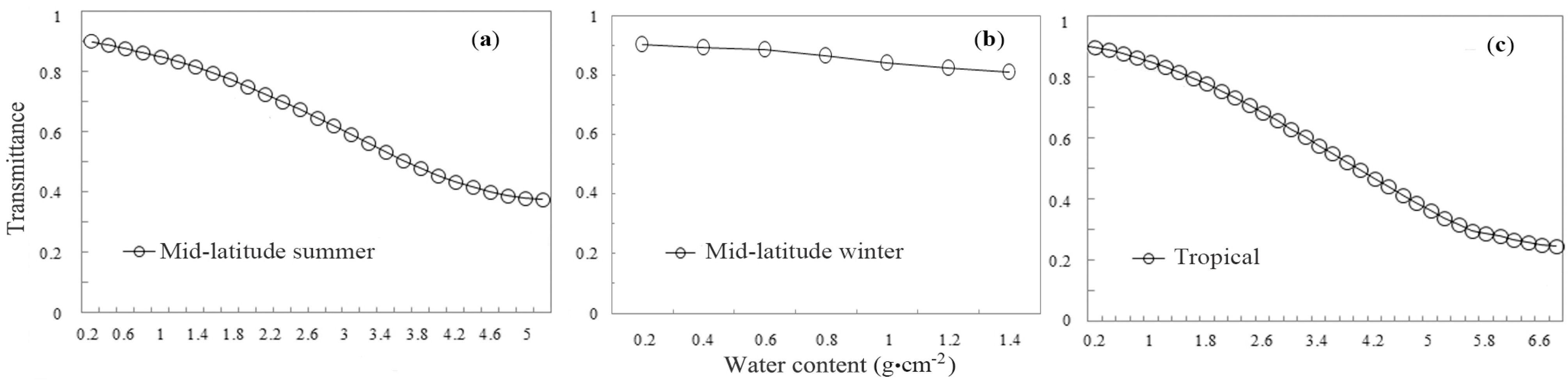
Table 5 shows the simulation results for the relationship between atmospheric transmittance and water vapor content. We plot the change of transmittance with water vapor content in
Figure 2, which indicates that the transmittance gradually decreases with water vapor content.
Table 5.
Change of atmospheric transmittance with water vapor content for Band 10 under various standard atmospheres.
Table 5.
Change of atmospheric transmittance with water vapor content for Band 10 under various standard atmospheres.
| Water Vapor Content (g·cm−2) | Tropical Atmosphere | Mid-Latitude Summer Atmosphere | Mid-Latitude Winter Atmosphere |
|---|
| 0.2 | 0.8966 | 0.8973 | 0.9034 |
| 0.4 | 0.8875 | 0.8884 | 0.8946 |
| 0.6 | 0.8769 | 0.8777 | 0.8827 |
| 0.8 | 0.8647 | 0.8650 | 0.8676 |
| 1.0 | 0.8507 | 0.8505 | 0.8495 |
| 1.2 | 0.8350 | 0.8340 | 0.8299 |
| 1.4 | 0.8176 | 0.8158 | 0.8205 |
| 1.6 | 0.7987 | 0.7958 | |
| 2.0 | 0.7564 | 0.7512 | |
| 2.4 | 0.7093 | 0.7013 | |
| 2.8 | 0.6585 | 0.6477 | |
| 3.2 | 0.6051 | 0.5915 | |
| 3.6 | 0.5503 | 0.5343 | |
| 4.0 | 0.4955 | 0.4804 | |
| 4.4 | 0.4415 | 0.4350 | |
| 4.8 | 0.3894 | 0.4015 | |
| 5.2 | 0.3400 | 0.3788 | |
| 5.6 | 0.2971 | | |
| 6.0 | 0.2778 | | |
| 6.4 | 0.2585 | | |
| 6.8 | 0.2457 | | |
Figure 2.
Change of atmospheric transmittance with water vapor content for Band 10 of Landsat 8 under various atmospheres: (a) mid-latitude summer; (b) mid-latitude winter; and (c) tropical.
Figure 2.
Change of atmospheric transmittance with water vapor content for Band 10 of Landsat 8 under various atmospheres: (a) mid-latitude summer; (b) mid-latitude winter; and (c) tropical.
Therefore, if we know the atmospheric water vapor content for the time when Landsat 8 passed over the sky of the study region, we are able to use
Table 5 for the estimation of atmospheric transmittance for LST retrieval. The estimation can be done through interpolation as follows:
where τ
10(
w) are the atmospheric transmittance of Band 10 for the atmosphere with water vapor content
w; τ
10(
w1), and τ
10(
w2) are the atmospheric transmittance of Band 10 at water vapor contents
w1 and
w2 given in
Table 5. In order to use the interpolation for atmospheric transmittance estimation, we have to select an atmosphere close to the atmospheric conditions of the study region. Then, we check
Table 5 to determine the location of the known water vapor content
w in the range of water vapor content shown in
Table 5. Finally, we apply Equation (13) for the atmospheric transmittance estimation.
Another approach for the estimation is to establish a function between the transmittance and the water vapor content. Since the change of the atmospheric transmittance with water vapor content is close to linearity in a certain range of water content change less than 2 g·cm
−2, we undertake the regression of transmittance to water vapor content shown in
Table 6, which indicates that all of the regression equations are statistically significant at a credential level of α = 0.01, and the determination coefficient
R2 is very high for all equations. Thus, the regression equations can be used to estimate atmospheric transmittance τ
10(
w) from the known water vapor content
w for the two thermal bands of Landsat 8 TIRS data. The standard estimation error (SEE) of the equations shows that the estimation has generally an accuracy of <0.01. The maximal regression coefficient of the equation is 0.133 for τ
10(
w) under mid-latitude atmosphere, which indicates that the possible error of estimation may be ~0.133 with the most likelihood water content estimation error of 1 g·cm
−2 [
16]. This error is very high. Therefore, accurate estimation of water vapor content is very important for accurate retrieval of LST from remote sensing data.
Table 6.
Estimation of atmospheric transmittance for the Landsat 8 TIRS bands. SEE, standard estimation error.
Table 6.
Estimation of atmospheric transmittance for the Landsat 8 TIRS bands. SEE, standard estimation error.
| Atmospheres | Water Vapor Content (g·cm−2) | Transmittance Estimation Equations | R2 | SEE |
|---|
| Mid-latitude summer | 0.2–1.6 | τ10 = 0.9184–0.0725 w | 0.983 | 0.0043 |
| | 1.6–4.4 | τ10 = 1.0163–0.1330 w | 0.999 | 0.0033 |
| | 4.4–5.4 | τ10 = 0.7029–0.0620 w | 0.966 | 0.0081 |
| Tropical model | 0.2–2.0 | τ10 = 0.9220–0.0780 w | 0.983 | 0.0059 |
| | 2.0–5.6 | τ10 = 1.0222–0.1310 w | 0.999 | 0.0033 |
| | 5.6–6.8 | τ10 = 0.5422–0.0440 w | 0.991 | 0.0017 |
| Mid-latitude winter | 0.2–1.4 | τ10 = 0.9228–0.0735 w | 0.988 | 0.0033 |
One problem in the estimation of atmospheric transmittance is that we are usually unable to obtain
in situ water vapor content for the images of Landsat 8. There are generally two ways to solve this problem. One is arbitrary estimate atmospheric water vapor content for the image according to the atmospheric conditions of the study region. Generally, the content can be arbitrarily given as 2.5 g·cm
−2 for clear sky in mid-latitude summer. Another is to use the air humidity data from a nearby atmospheric observation station in the imaging region. Suppose we are able to obtain air humidity (H) and air temperature (T
a) from the station; water vapor content in the atmospheric column up to satellite altitude can be estimated as follows:
where
w is total water vapor content (g·cm
−2) in the atmospheric column up to the sensor,
w(0) is the water vapor content (g·cm
−2) at the ground of the atmosphere and
Rw(0) is the ratio of water vapor content at the first layer to the total. The ratio may differ for different atmospheres, with
Rw(0) = 0.6834 for tropical atmosphere,
Rw(0) = 0.6819 and
Rw(0) = 0.6593 for subtropical summer and winter atmospheres, respectively, and
Rw(0) = 0.6834 and
Rw(0) = 0.6356 for mid-latitude summer and winter atmospheres, respectively [
16]. The water vapor content at the ground can be computed as:
where
H is air humidity (%) at the ground,
E is the saturation mix ratio (g/kg) of water vapor and air for a specific air temperature and
A is the air density (g/m
3) at the specific air temperature.
Table 7 gives the saturation mix ratio and air temperature for various temperatures. Thus, if we have an air temperature of 33.7 °C and an air humidity of 56% for the sub-tropical region in the summer season, we have
w(0) = 56 × 34.38 × 1.151/1000 = 2.217 g·cm
−2 and
w = 2.217/0.681924 = 3.2517 g·cm
−2.
Table 7.
Air density (A) and saturation mix ratio (E) of water vapor to air for various air temperatures (T).
Table 7.
Air density (A) and saturation mix ratio (E) of water vapor to air for various air temperatures (T).
| T (°C) | 45 | 40 | 35 | 30 | 25 | 20 | 15 | 10 | 5 | 0 | −5 | −10 |
|---|
| E (g·kg−1) | 66.33 | 49.81 | 37.25 | 27.69 | 20.44 | 14.95 | 10.83 | 7.76 | 5.50 | 3.84 | 2.52 | 1.63 |
| A (kg·m−3) | 1.11 | 1.13 | 1.15 | 1.17 | 1.18 | 1.21 | 1.23 | 1.25 | 1.27 | 1.29 | 1.32 | 1.34 |
6. Determination of Ground Emissivity
It is well known that the emissivity of an object is mainly determined by its thermo-physical characteristics. For the ground surface, the components composing the surface are the main factors determining the ground emissivity [
33,
34,
35]. Many effective methods have been approved to estimate the emissivity for LST retrieval [
36,
37]. Since the emissivity is variable with the wavelength, the NDVI threshold method (NTM) [
38] can be used to estimate the emissivity of different land surfaces in the 10–12 µm range. Additionally, the spectral range of Band 10 of Landsat 8 is suitable in this range. At this wavelength range, the emissivity could be modeled as follows [
38]:
Subject to:
where ε
λ is the band emissivity, ε
vλ and ε
sλ are respectively the vegetation and soil emissivity,
Pv is the proportion of vegetation,
C is a term due to surface roughness (
C = 0 for a flat surface), NDVI
v and NDVI
s are the NDVI for a fully vegetated pixel and a soil one, respectively, and
F' is a geometrical factor ranging between zero and one.
Usually, the vegetation cover fraction at the pixel scale can be computed from its NDVI as follows [
39,
40]:
Over particular areas, NDVI
v and NDVI
s values can be extracted from the NDVI histogram. Values of NDVI
v = 0.5 and NDVI
s = 0.2 were proposed to apply in global conditions [
38]. While the value for vegetated surfaces (NDVI
v = 0.5) may be too low in some cases, for higher resolution data over agricultural sites, the NDVI
v can reach 0.8 or 0.9 [
41].
The emissivity of water bodies is quite stable in comparison with land surfaces. It only has a slight change with the mixture of sediments or biomass in the water. Then, using the ASTER spectral database [
42], we get the average emissivity of four representative terrestrial materials in Band 10 and Band 11 of Landsat 8, as shown in
Table 8.
Table 8.
Emissivity of representative terrestrial materials for the Landsat 8 TIRS Band 10.
Table 8.
Emissivity of representative terrestrial materials for the Landsat 8 TIRS Band 10.
| Terrestrial Material | Water | Building | Soil | Vegetation |
|---|
| Emissivity | 0.991 | 0.962 | 0.966 | 0.973 |
7. Sensitivity Analysis of the Algorithm
Due to many difficulties, such as the unavailability of precise profile data about the atmosphere and the complexity of the emitted ground surface in terms of material composition, the determination of these three critical parameters will unavoidably involve some errors, which consequently will lead to the error in LST retrieved by the algorithm. Therefore, it is very necessary to conduct sensitivity analysis of the algorithm in order to assess the impacts of the possible estimation error of these critical parameters on the possible LST estimation error by the algorithm. For convenience, the following formula is used to express the possible LST estimation error of the algorithm [
16]:
where Δ
Ts is the LST estimation error of our algorithm due to the possible error in variable
x, which is the effective mean atmospheric temperature, ground emissivity and atmospheric transmittance in our case. Thus, Δ
x represents the possible error of variable
x.
Ts(
x + Δ
x) and
Ts(
x) are the LSTs computed by our algorithm in Equation (19) for
x + Δ
x and
x, respectively.
The performance of the sensitivity analysis for the algorithm requires several conditions to be assumed. Since the analysis is mainly focused on the variables of ground emissivity, atmospheric transmittance and effective mean atmospheric temperature, we need to assume what is known of each of the variables. For example, atmospheric transmittance needs to be determined for sensitivity analysis of the ground emissivity, and vice versa. The overpass of Landsat 8 in many regions is at about 10:30 a.m. local time. The near surface air temperature is assumed to be ~25 °C and water vapor content to be ~2 g·cm−2. Atmospheric transmittance is estimated from the atmospheric water vapor content. Thus, we assume the water vapor content to be 2 g·cm−2 for the analysis of ground emissivity. For the water vapor content of 2 g·cm−2, atmospheric transmittance will be 0.75 for Landsat 8 TIRS Band 10 in the mid-latitude atmosphere. For the sensitivity analysis of atmospheric transmittance, we assume the ground emissivity to be 0.97 for the general case. Additionally, the LST under those conditions is assumed to be from ~20 °C to ~40 °C.
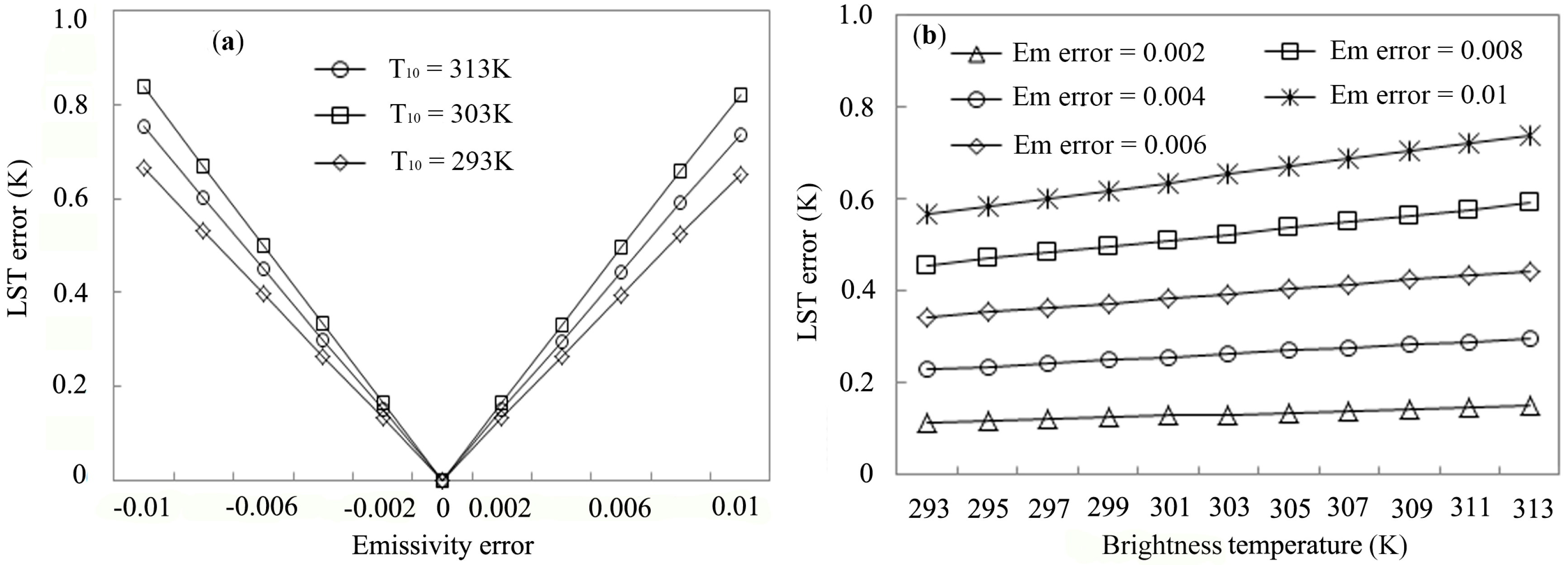
Figure 3 illustrates the probable LST estimation error of our algorithm due to the possible ground emissivity estimation error. Thus, we average the LST error for the temperature difference and the temperature ranges and focus on its change with the possible estimation errors in ground emissivity, which gives the change of the LST error shown in
Figure 3a. In order to assess the impact of ground emissivity estimation error on possible LST error, we consider the possible emissivity error from −0.01 to 0.01, which represent two extremes of the estimation error. Research has shown the error in estimation of ground emissivity usually to be ≤0.006 [
16]. In this case, the possible LST error is ~0.4 K for the estimation. While the same emissivity error may result in different LST estimation error for different brightness temperatures, the LST error will increase with the brightness temperature under the same emissivity error. However, the maximum LST error increases about only 0.1 K with the brightness temperature increase from 20 K to 293 K, as shown in
Figure 3b.
Figure 3.
Probable LST estimation error of the improved mono-window IMW algorithm due to the possible error in emissivity estimation. (a) Average LST error against possible emissivity error in Band 10; (b) possible LST error against Band 10 brightness temperature for different emissivity errors of Landsat 8 TIRS data.
Liston and Elder have indicated that the error of spatialized air humidity is usually smaller than ±5% at a regional scale [
29], such as the size of a Landsat image scene (185 km × 185 km). Thus, it can be expected that the error in water content estimation might probably be in the range of ±0.3 g·cm
−2, with a maximum of ±0.3 g·cm
−2. With this consideration, we conducted our simulation on the effect of possible error in atmospheric water content on LST retrieval. We respectively simulated the water content of 2 g·cm
−2, 3 g·cm
−2 and 4 g·cm
−2 with an error of ±0.5 g·cm
−2 as the maximum.
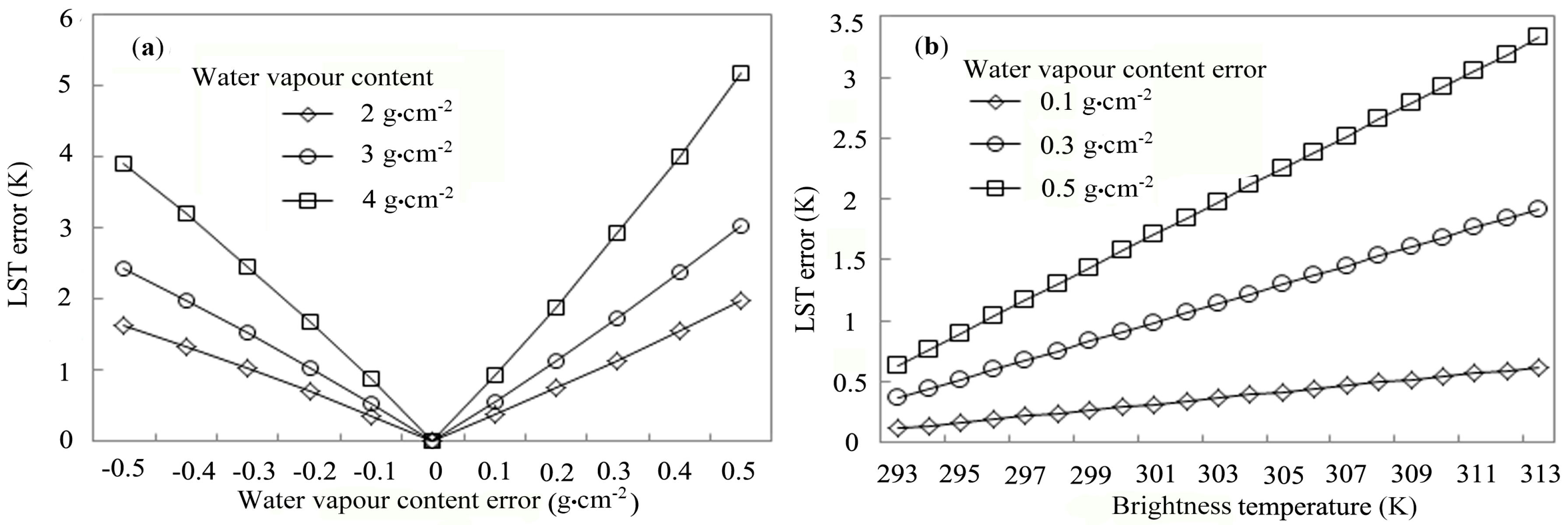
Figure 4a indicates that LST estimation error increases remarkably with water content error. With the water content of 3 g·cm
−2, the LST error is 1 K for an error of 0.02 g·cm
−2 in water content estimation. This is a very sensible response to emissivity error in the LST retrieval. The LST error increases obviously with brightness temperature under the same water content error. Under the water content error at 0.5 g·cm
−2, the LST error increases ~3 K with the brightness temperature increase from 20 K to 293 K, as shown in
Figure 4b. Therefore, the LST retrieval error will become much more sensible when the brightness increases with water content estimation error and the emissivity error. However, the error of water content is under 0.3 g·cm
−2 for most situations, so the LST error is about 1 K.
Figure 4.
Probable LST estimation error of the IMW algorithm due to the possible error in atmospheric water content estimation. (a) Average LST error against possible water content error in Band 10; (b) possible LST error against Band 10 brightness temperature for different the water content error of Landsat 8 TIRS data.
The effective mean atmospheric temperature error to LST error is very affected by the parameter
D10/
C10 according to Equation (3). We compute the ratio of
D10 to
C10 for several combinations. The results are given in
Table 9. The ratio changes about 0.02 with the emissivity changing from 0.96 to 0.99 under the same transmission of 0.7. However, it changes by about 0.34 with the transmission changing from 0.7 to 0.9 under the same transmission of 0.96. Therefore, the ratio
D10/
C10 is mainly dependent on transmittance, though emissivity has a slight effect on it.
Table 9.
Comparison of the ratio D10/C10 for different combinations.
Table 9.
Comparison of the ratio D10/C10 for different combinations.
| Emissivity | Transmission | Parameter C10 | Parameter D10 | Ratio D10/C10 | Average Ratio |
|---|
| 0.96 | 0.7 | 0.672 | 0.3084 | 0.4589 | 0.4116 |
| 0.97 | 0.7 | 0.679 | 0.3063 | 0.4511 | |
| 0.98 | 0.7 | 0.686 | 0.3042 | 0.4434 |
| 0.99 | 0.7 | 0.693 | 0.3021 | 0.4359 |
| 0.96 | 0.8 | 0.768 | 0.2064 | 0.2688 | 0.2616 |
| 0.97 | 0.8 | 0.776 | 0.2048 | 0.2639 | |
| 0.98 | 0.8 | 0.784 | 0.2032 | 0.2592 |
| 0.99 | 0.8 | 0.792 | 0.2016 | 0.2545 |
| 0.96 | 0.9 | 0.864 | 0.1036 | 0.1199 | 0.1166 |
| 0.97 | 0.9 | 0.873 | 0.1027 | 0.1176 | |
| 0.98 | 0.9 | 0.882 | 0.1018 | 0.1154 |
| 0.99 | 0.9 | 0.891 | 0.1009 | 0.1132 |
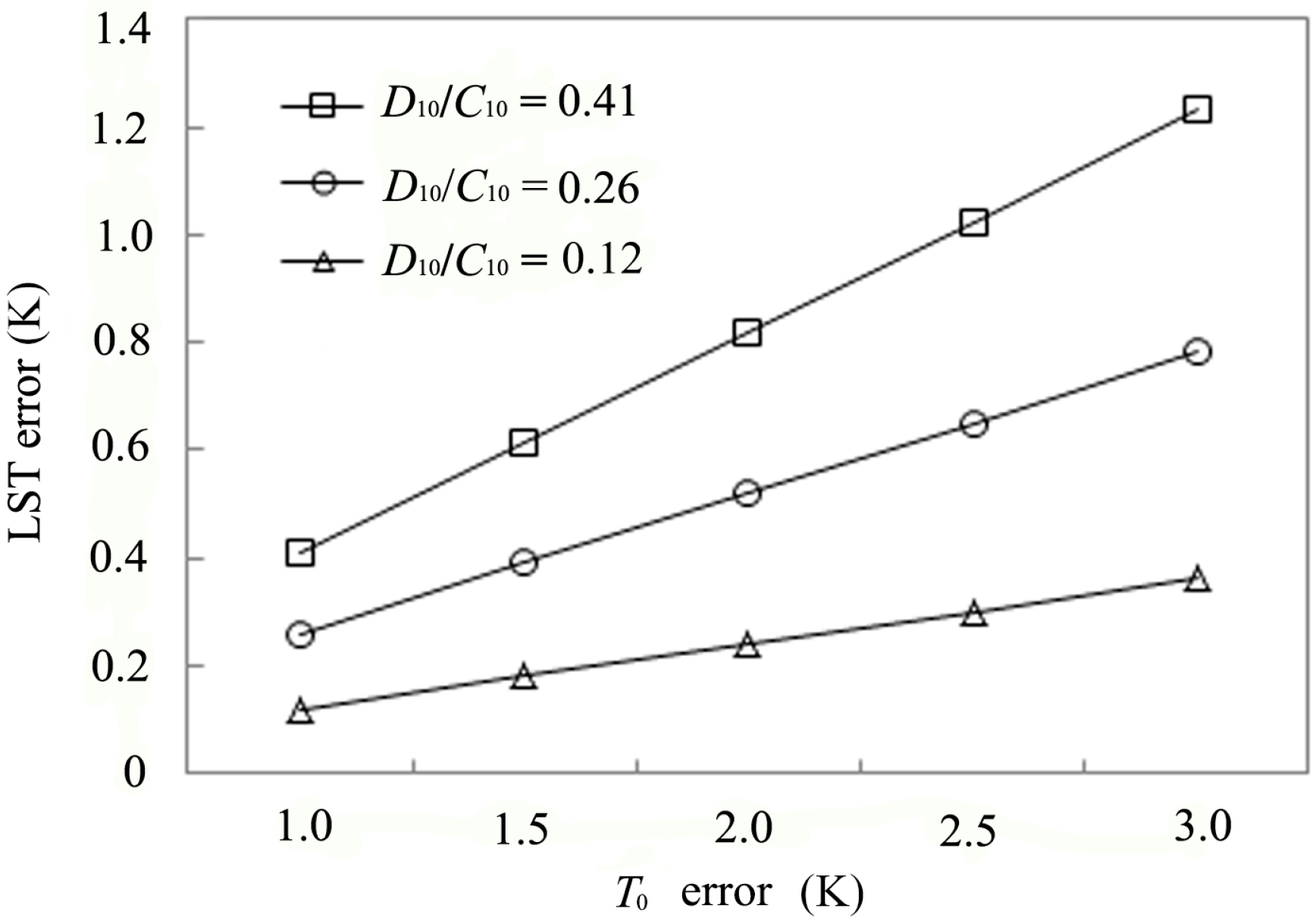
The LST error will increase with the effective mean atmospheric temperature error, as shown in
Figure 5. For a Landsat8 image covered region, the error of near surface air temperature (
T0) spatialized with meteorological data and DEM data is smaller than 3 K under the more than four meteorological stations situation [
26]; the
Ta error is smaller than 2.7 K for most situations according to the relationship between effective mean atmospheric temperature and air temperature near the surface. Thus, it can be concluded that the moderate LST error of the
Ta is about 0.4 K with the ratio D
10/C
10 of 0.26 and the
T0 error of 1.5 K.
Figure 5.
Probable LST estimation error of the IMW algorithm due to the possible error in near surface air temperature estimation.
Figure 5.
Probable LST estimation error of the IMW algorithm due to the possible error in near surface air temperature estimation.
Sensitivity analysis conducted for the IMW algorithm reveals that the possible error in estimating the required atmospheric water content has relatively the highest impact on the probable LST estimation error. Under moderate errors in both water vapor content and ground emissivity, the algorithm may be able to have an accuracy of ~1.4 K for LST retrieval.
8. Comparison between IMW and SC Algorithms
The best way to validate the algorithm is to compare the
in situ ground truth measurements of LST with the retrieved ones. However, it is extremely difficult to carry out such measurements over the short time of the satellite pass. Atmospheric simulation programs, such as MODTRAN, are usually used for validation of LST algorithms due to the high approximation through simulation of satellite-observed thermal radiance reaching the sensor at the satellite platform. Thus, we validate our IMW algorithm and compare it with the SC algorithm through simulation of the thermal radiance transfer process for Landsat 8 TIRS using MODTRAN 4.0 [
32].
A number of situations are designed for the validation. Three main atmosphere models (tropical model, mid-latitude summer model, mid-latitude winter model) are chosen to validate the algorithm. The water content and the near surface air temperature are respectively 4.1 g·cm
−2 and 26.5 °C for the tropical model in MODTRAN 4.0; the possible LST under this atmosphere may range from 30 °C–60 °C, and four LSTs (30 °C, 40 °C, 50 °C, and 60 °C) are assumed for the simulation. For the mid-latitude summer model, the water content and the near surface air temperature are respectively 2.9 g·cm
−2 and 21.0 °C, and the simulated LSTs are 20 °C, 30 °C, 40 °C and 50°C. Additionally, for the mid-latitude winter model, the water content and the near surface air temperature are respectively 0.85 g·cm
−2 and −1.1 °C, and the simulated LSTs are −5 °C, 5 °C and 15 °C. Here, we mainly present the results for the three atmosphere models with emissivity cases of 0.97.
Table 10 gives the simulation outputs of MODTRAN 4.0 for various atmosphere models and the difference between the retrieved LSTs and the simulated ones. The average accuracy of the algorithm is 0.67 K, and the RMSE is 0.43 K for LST retrieval. This good matching of the retrieved LSTs to the simulated ones confirms the applicability of our algorithm for LST retrieval from Landsat 8 TIRS data.
Table 10.
Main results of testing the IMW algorithm for various situations.
Table 10.
Main results of testing the IMW algorithm for various situations.
| Atmosphere Model | TS (°C) | Ta (°C) | Emissivity | Transmittance | B10(T10) (W·m−2 sr−1·μm−1) | T10 (K) | Retrieved
(K) | | − TS| (K) |
|---|
| Mid-latitude summer | 20 | 15.34 | 0.97 | 0.6276 | 8.2253 | 289.96 | 292.09 | 1.07 |
| 30 | 15.34 | 0.97 | 0.6276 | 9.0904 | 296.39 | 302.59 | 0.57 |
| 40 | 15.34 | 0.97 | 0.6276 | 10.0278 | 302.99 | 313.35 | 0.19 |
| 50 | 15.34 | 0.97 | 0.6276 | 11.0498 | 309.79 | 324.45 | 1.29 |
| Tropical | 30 | 19.69 | 0.97 | 0.4829 | 9.1273 | 296.66 | 301.91 | 1.25 |
| 40 | 19.69 | 0.97 | 0.4829 | 9.8523 | 301.78 | 312.80 | 0.36 |
| 50 | 19.69 | 0.97 | 0.4829 | 10.6339 | 307.06 | 324.04 | 0.88 |
| 60 | 19.69 | 0.97 | 0.4829 | 11.3698 | 311.85 | 334.21 | 1.05 |
| Mid-latitude winter | −5 | −5.87 | 0.97 | 0.8602 | 5.4824 | 266.44 | 267.68 | 0.48 |
| 5 | −5.87 | 0.97 | 0.8602 | 6.4142 | 275.08 | 277.91 | 0.25 |
| 15 | −5.87 | 0.97 | 0.8602 | 7.4386 | 283.76 | 288.18 | 0.02 |
| Average error | | | | | | | | 0.67 |
| RMSE | | | | | | | | 0.43 |
The SC algorithm developed by Jiménez-Muñoz
et al. [
12] has been tested through more than 4000 atmospheric profiles in the Thermodynamic Initial Guess Retrieval (TIGR) dataset. Testing results indicate that the SC algorithm in total provides about a −1.5 K LST retrieval error with atmospheric profiles with water vapor content less than 3 g·cm
−2 and more than a −4 K LST retrieval error when water vapor content is higher than 3 g·cm
−2. For the restriction of data acquisition, we could not compare the IMW algorithm with the SC algorithm through so many atmospheric profiles. Thus, three main atmospheric profiles in MODTRAN are chosen to compare our IMW algorithm with the SC algorithm.
Table 11 gives the LST retrieval errors of the two algorithms. As shown in
Table 11, the LST retrieval results of the IMW algorithm are better than the SC algorithm under all assumed situations of the three atmospheric profiles. The average error and RMSE of the IMW algorithm are −0.05 K and 0.84 K, respectively; much less than the −2.86 K and 1.05 K of the SC algorithm.
Table 11.
Comparing LST retrieval errors of the IMW and single-channel (SC) algorithms for various situations.
Table 11.
Comparing LST retrieval errors of the IMW and single-channel (SC) algorithms for various situations.
| Atmosphere Model | TS (°C) | w (g·cm−2) | SC (K) | IMW (K) |
|---|
| Mid-latitude summer | 20 | 2.9 | −2.37 | −1.07 |
| 30 | 2.9 | −2.94 | −0.57 |
| 40 | 2.9 | −3.42 | 0.19 |
| 50 | 2.9 | −3.73 | 1.29 |
| Tropical | 30 | 4.1 | −2.28 | −1.25 |
| 40 | 4.1 | −2.95 | −0.36 |
| 50 | 4.1 | −3.48 | 0.88 |
| 60 | 4.1 | −5.01 | 1.05 |
| Mid-latitude winter | −5 | 0.85 | −1.18 | −0.48 |
| 5 | 0.85 | −1.74 | −0.25 |
| 15 | 0.85 | −2.32 | 0.02 |
| Average error | | | −2.86 | −0.05 |
| RMSE | | | 1.05 | 0.84 |
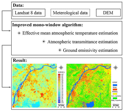
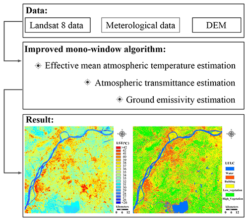
9. Application of the Algorithm to Nanjing and Its Vicinity in East China
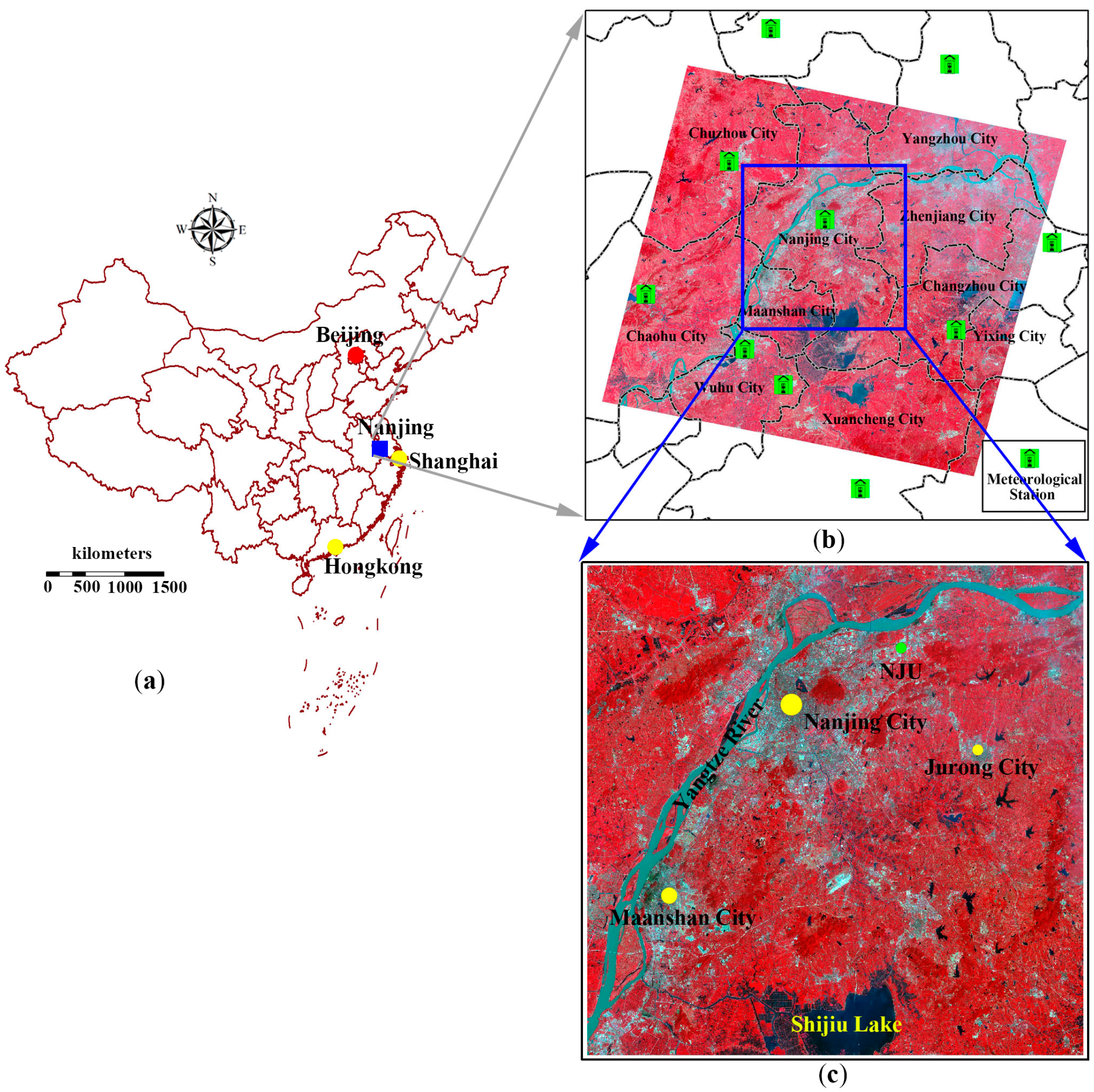
In order to provide an example of applying the algorithm to the real world for LST retrieval, we use it to retrieve LST from the Landsat 8 TIRS data of Nanjing and its vicinity in east China, as shown in
Figure 6a. Nanjing has long been recognized as one of China’s “Four Furnaces” (the other three are Wuhan, Chongqing and Nanchang) along the Yangtze River Basin [
43]. Characterized by a typical subtropical monsoon climate, the region has an average annual rainfall of 1200 mm. The mean monthly air temperature of the region ranges from ~1 °C in January to ~30 °C in July, with an annual average of approximately 15.4 °C. With the rapid development of economy, urbanization is very obvious in the region, especially Nanjing City. In recent years, the developed area in Nanjing City has expanded significantly, from 515 km
2 in 2000 to 1311 km
2 in 2012. The percentage of the developed area to the total increased from 15.4% in 2000 to 39.2% in 2012. The dramatic expansion of the developed area has had a remarkable effect on the urban environment in the region. The phenomenon of the urban heat island (UHI) effect has become more and more severe in the region in recent decades [
44].
Figure 6.
Application of the algorithm to Nanjing and its vicinity in east China. (a) The geographic location of Nanjing and its vicinity in China; (b) the spatial distribution of meteorological stations around the region; (c) pseudo-color composite (RGB: 5, 4, 3) of Landsat 8 OLI data of the region.
LST retrieved from satellite TIR data has commonly been used as an important indicator to study the effect of UHI at the regional scale. In the study, we apply our IMW algorithm to Landsat 8 TIRS band data for LST retrieval in the region. The Landsat 8 images used for the LST retrieval in the region were acquired on 11 August 2013 at 10:39:22 a.m. local time. We obtained the image from the website of the USGS Earth Resource Observation Systems Data Center. Radiometric and geometric corrections have been done to the image, which has a Universal Transverse Mercator coordinate system with the WGS-84 datum.
Figure 6c shows the false color composite (RGB: 5, 4, 3) of Landsat 8 Operational Land Imager (OLI) data. Yangtze River, the famous big river in China, runs through the region from southwest to northeast. Several lakes can also be clearly seen in the image, and the biggest one is Shijiu Lake in the south of the image. Since the imaging date is in the summer, vegetation in the region is very dense, with an average cover fraction of 80% for most areas, except the developed areas. There are 10 meteorological stations around this region, as shown in
Figure 6b. With the available air relative humidity and air temperature near the surface, we can acquire the effective mean atmospheric temperature and water content for each pixel of the image. After estimating the ground emissivity by the Landsat 8 VNIR bands, we retrieved the LST from the image.
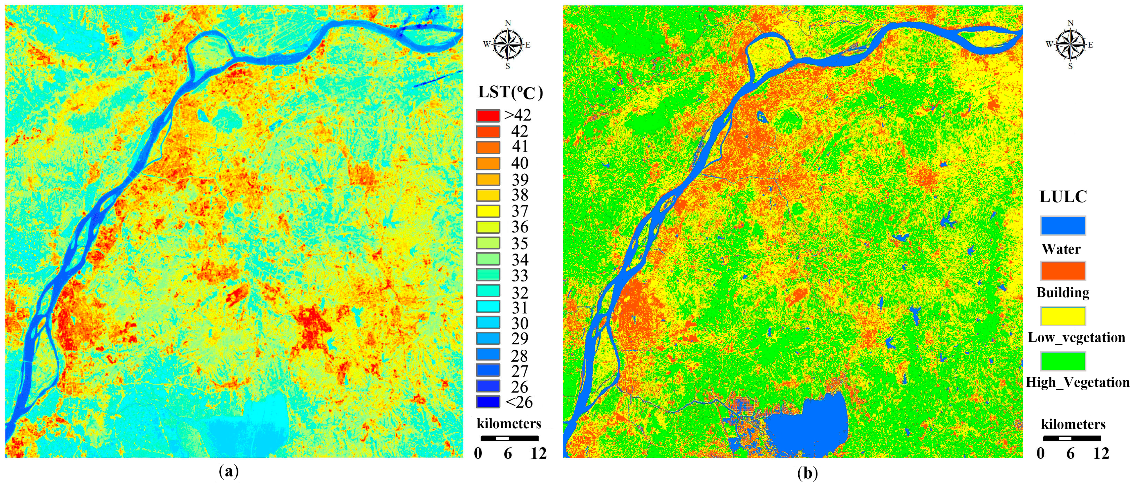
Before using the IMW algorithm, we need to estimate the essential parameters: ground emissivity is estimated by the land use and land cover (LULC) shown in the
Figure 7b data; atmospheric transmittance is calibrated by the air relative humid data in the meteorological data; and the effective mean atmospheric temperature is estimated by the spatialized air temperature with meteorological data and topography data. Then, we are able to retrieve the LST from Landsat 8 TIRS Band 10 data.
Figure 7a shows the spatial distribution of the retrieved LST. It can be seen from
Figure 7a that LST in the region ranged from 26 °C to 42 °C with a mean of 37.6 °C. The developed area in the region has very high LST, usually above ≥40 °C. Several high LST centers can be easily identified, which include Nanjing and Ma’anshan cities. Specifically, Nanjing City has an average LST of 40.2 °C. Another feature of LST distribution in the region is that the areas along the Yangtze River have very high LST due to the fact that these areas are mainly the developed areas of Nanjing and Ma’anshan cities. Water bodies in the region, especially the Yangtze River, have the lowest LST due to the strongest cooling process as a result of evaporation over the water surface. The suburban areas in the region usually have an LST of 38 °C. Thus, the LST difference between the developed area and the suburban area in the region may be high, up to ~8 K in the imaging date, implying that the intensity of UHI is much higher than the average [
43,
44]. This extremely high UHI effect revealed by the LST image provides another direct piece of evidence to support the traditional saying that Nanjing is one of the notorious “Four Furnaces” along the Yangtze River Basin.
Figure 7.
(a) The retrieved LST image retrieved by the mono-window algorithm with Band 10 of the region on August 11, 2013; (b) the land use and land cover (LULC) map.
Figure 7.
(a) The retrieved LST image retrieved by the mono-window algorithm with Band 10 of the region on August 11, 2013; (b) the land use and land cover (LULC) map.
10. Conclusions
An attempt has been made in this study to develop an IMW algorithm for LST retrieval from the Landsat 8 TIRS data. The algorithm was derived from the instantaneous radiative transfer equations describing the observed thermal radiance of the TIR Band 10 of Landsat 8 TIRS. We followed the approach of the mono-window algorithm to solve the instantaneous equations for our algorithm development. Three essential parameters (effective mean atmospheric temperature, ground emissivity and atmospheric transmittance) are required for LST retrieval by the IMW algorithm. Methods to determine the required essential parameters are also presented with details in the study, which makes the application of the algorithm to the real world easy. The ground emissivity is estimated through the land cover pattern from other band data of the Landsat 8, and the other two parameters are estimated by the climatological-based parameters.
It is very difficult to obtain an accurate estimate of ground emissivity. Such an estimate usually has an error of about ±0.006 for most cases. Results from our sensitivity analysis indicate that such an error in ground emissivity estimation may lead to an error of 0.4 K in LST retrieval by the proposed IMW algorithm. Water vapor content is usually a sensitive parameter in traditional LST retrieval methods. The water vapor content is estimated with an error of ±0.3 g·cm2, which is reasonable for most situations. Additionally, the error of retrieved LST from the water vapor content error is ~1 K. We can conclude that the LST retrieval method is sensitive to water vapor content estimated error. The effective mean atmosphere temperature error is mainly decided by the ratio D10/C10 computed by emissivity and transmission. Additionally, for most situations, the error of retrieved LST from the effective mean atmosphere temperature is ~0.4 K. Thus, it can be said that, under moderate errors in both water vapor content and ground emissivity estimations, the algorithm may be able to have an accuracy of ~1.4 K for LST retrieval.
The IMW algorithm has been successfully applied to Nanjing and its vicinity in east China as an example for analyzing the spatial distribution of LST differences. Comparison of the retrieved LST from TIRS Band 10 by the IMW algorithm with those by the SC algorithm suggests that the average error and RMSE of the IMW algorithm are −0.05 K and 0.84 K, respectively, which are much less than the −2.86 K and 1.05 K of the SC algorithm. Results from the application indicate that the IMW algorithm is very good at understanding the natural urban heat island. The spatial distribution of LST in the region is quite well matched with the land surface covers. The successful application of the IMW algorithm confirms that the improved mono-window algorithm can be used as an efficient method to retrieve the LST from the Landsat 8 TIRS data.


