A Novel Technique for Time-Centric Analysis of Massive Remotely-Sensed Datasets

Abstract

Analyzing massive remotely-sensed datasets presents formidable challenges. The volume of satellite imagery collected often outpaces analytical capabilities, however thorough analyses of complete datasets may provide new insights into processes that would otherwise be unseen. In this study we present a novel, object-oriented approach to storing, retrieving, and analyzing large remotely-sensed datasets. The objective is to provide a new structure for scalable storage and rapid, Internet-based analysis of climatology data. The concept of a “data rod” is introduced, a conceptual data object that organizes time-series information into a temporally-oriented vertical column at any given location. To demonstrate one possible use, we ingest 25 years of Greenland imagery into a series of pure-object databases, then retrieve and analyze the data. The results provide a basis for evaluating the database performance and scientific analysis capabilities. The project succeeds in demonstrating the effectiveness of the prototype database architecture and analysis approach, not because new scientific information is discovered, but because quality control issues are revealed in the source data that had gone undetected for years.

1. Introduction

Online libraries of remotely-sensed earth observations keep growing every year, in some cases exponentially. Climate scientists now have more data than ever, but the process of retrieving, filtering, and analyzing it can be slow and cumbersome. In particular, data exploration and time-series analysis, especially important for climate studies, is hampered by the native format of the data: Most imagery is stored as separate, georeferenced files for single dates that must be combined to perform a time-series analysis. Some of these limitations can be overcome by reorganizing the data into portable, self-describing data formats such as Network Common Data Form (NetCDF) or Hierarchical Data Format (HDF). However, for studies that want to analyze the entirety of a massive remotely-sensed dataset, perhaps gigabytes or terabytes in size, downloading and processing data in these formats is often impractical.

The “Data Rods” project was conceived to demonstrate a new system for rapid, scalable management and analysis of time-centric data across massive datasets. The essence of the project was to host several large, remotely-sensed datasets in a series of scalable databases, and then demonstrate how they could be used to enable high-speed, time-centric scientific analyses. Budget and hardware constraints were also considered relevant, so we limited the hardware to a single server.

In our project, a data rod is a conceptual data object, containing a time-series of data at a specific set of gridded coordinates. (Please note that the terms “object” and “object-oriented” in this article refer to software engineering design methodologies rather than segmentation and classification image processing techniques). Ideally, a single data rod encapsulates all the information known at one location through time. This approach fundamentally reorients imagery from a spatial format into a time-centric orientation. Typically, the information contained in a data rod will be image pixels, such as multispectral or hyperspectral data, or derived types such as surface temperature or albedo.

Although our source data was generally gridded imagery, the system was intended primarily for time-centric filtering and statistical analyses, not image processing. For instance, a researcher wishing to find data anomalies or trends at a geographic point through time would only need to specify the location, query terms, and desired analysis functions. All processing would occur on a remote server. The results would be reported automatically, but the user would also have the option of downloading the raw pixel data.

The Data Rods project proposed to store collections of data rods in stand-alone or distributed databases, providing users with immediate access to large collections of remotely-sensed data (as opposed to only allowing direct access to the metadata). Temporal data analyses could then be performed by querying for the set of data rods that cover the spatial area of interest. This query process would implicitly retrieve only the data necessary for the desired analysis, avoiding the overhead of downloading extraneous data. Combined with server-side processing and user-friendly analytical tools, the project’s overarching objective was to reduce the research cycle time from weeks or months down to days, perhaps less.

Before settling on a database, we evaluated a spectrum of data storage options. Storing the data entirely as arrays within RAM provided the fastest response and most flexibility, but scalability was problematic: To host a single terabyte-scale dataset, much less multiple different datasets of that size, would have exceeded our hardware resource limitations. Storing the data as simple files on a hard disk was the most economical approach, but then the query tools would have to be programmed from scratch for each data type. A powerful database, however, could potentially provide an economical solution, offering both scalability and query flexibility.

The development of efficient, highly-functional databases was therefore at the heart of the Data Rods project. To prove its utility, the project needed to demonstrate a rapid, server-side scientific analysis using the databases. This paper describes the dataset used, the database construction, and a demonstration analysis. The cryospheric data we selected was downloaded from the National Snow and Ice Data Center (NSIDC); we chose a 25-year collection of daily Greenland satellite imagery as our example dataset. Despite the limited spatial extent of the initial dataset, the Data Rods project aimed for data storage and retrieval techniques that could be expanded to continental scales and be broadly applicable other fields of research. By analyzing the entirety of the dataset, we were also seeking to reveal patterns or processes occurring on the Greenland Ice Sheet (GrIS) that had heretofore gone undetected, i.e., taking a “big data analytics” approach to processing a massive, temporally-oriented dataset. In this regard the project was successful because the results revealed unexpected quality control problems in the original data.

2. Data

For our demonstration dataset, we chose the NOAA/NASA Polar Pathfinder program’s Advanced Very High Resolution Radiometer (AVHRR) data, available from a variety of sources at different processing levels. NOAA satellites carrying AVHRR sensors have been on orbit since 1978; the capabilities of the AVHRR radiometers have varied only slightly over the years, and the polar orbits have remained roughly the same, providing a uniquely long-term view of the Earth’s polar regions. A consistent dataset of this kind is ideal for longer-term climatological studies.

The AVHRR Polar Pathfinder (APP) dataset was obtained from NSIDC as a post-processed, calibrated and gridded level-3/4 product at a 5 km resolution (25 km² per grid cell) [1,2]. The APP dataset contained imagery from 1981 to 2005, and had been available to the scientific community since 2005, with a processing update in 2008. Along with multispectral imagery, the dataset also included several derived data types such as skin temperature, albedo, and cloud masks.

Any long-term dataset that spans multiple satellites will likely include intervals when the data is missing or of poor quality. NASA and NSIDC provided a Completeness Report detailing the dates and causes of known bad or missing APP data; those dates were eliminated from consideration in this study.

In addition to the APP dataset, an additional database was created that contained a Land-Surface-Coastline-Ice (LOCI) mask [3]. This second dataset was used to constrain the analysis to the Greenland ice sheet.

Albedo Data

The analysis portion of our study used the APP broadband surface albedos. A brief explanation of the albedo data is given here to clarify the quality problems later found during the analysis.

Albedo is defined as the net reflectance of incident sunlight, and it effectively controls the amount of solar energy absorbed by the ice sheet [4,5]. In response, the absorbed light affects the overall energy balance, with positive feedbacks that may increase melting [6]. Thus, any significant trend in the albedo is important in predicting the future of the GrIS [7]. The definition of albedo can be further sub-defined as either narrowband, i.e., a spectral albedo that characterizes only portions of the solar spectrum, or broadband, that considers the broader spectrum of incident light. The albedos provided in the APP dataset are broadband, with a bandwidth of approximately 0.3–3.5 μm [4].

Albedo is measured on a scale between zero (no reflectance) and one (total reflectance), or as a percentage. The clear-sky broadband surface albedo of dry snow ranges between 0.70 and 0.90, with typical values for both satellite and ground measurements in the neighborhood of 0.80 to 0.85 [8,9,10,11]. Melting snow is much more variable and dependent on water content, where albedos may drop below 0.60 [12]. At high altitude locations on the GrIS, where there is frequent snowfall and melting is rare, the albedo should remain near 0.80 or higher.

Surface albedo is a measure of hemispherical reflectance. However, satellites measure instantaneous top-of-atmosphere (TOA) radiances from a single viewpoint, with the optical depth of an intervening atmosphere. Thus, surface albedo cannot be directly measured by satellite; it must be modeled and constructed from radiance measurements. And because snow and ice reflect anisotropically, the solar zenith angle and viewing geometry between the satellite, Sun, and the Earth’s surface further complicate satellite-derived measurements of albedo [13,14]. Additionally, the AVHRR sensors have discrete bandwidths and response characteristics, so broadband reflectance measurements must be approximated using calibrated narrowband radiances in the visible and near-IR spectrum, AVHRR channels 1 and 2 respectively. The APP surface albedos were generated from the these channels using a software package called the Cloud And Surface Parameter Retrieval (CASPR) system [15]. Since visible light is necessary for deriving albedo, values calculated during months with low sun angles (or no sun at all, for high latitudes) can be very noisy. To ensure data quality, this study was limited to the summer months of May through August.

Given the modeling steps and assumptions necessary to calculate surface albedos from satellite data, the values are prone to significant errors [4,16,17]. Sources of error include the presence of clouds, errors in the angular reflection models, variations in the sun-satellite geometry, atmospheric optical depth uncertainties, and sensor calibrations. The differences between in situ and satellite observations of clear-sky albedos over the GrIS have been explored by Stroeve et al. [17,18]. The in situ observations originated from 15 Greenland Climate Network (GC-Net) Automated Weather Stations on the Greenland Ice Sheet [19]. Using data from 1993 to 1998, AVHRR-derived surface albedos were found to average about 10% less than the in situ measurements, although variations in instrumentation bandwidths explain some of the difference. Accounting for the instrumentation bias, the errors between the satellite and in situ albedos typically average closer to 6%.

3. Database Construction

This study’s objective was to facilitate time-series analyses. In the event that all possible analysis questions are known beforehand, datasets can be organized into highly efficient flat files, eliminating any advantage to using a database. On the other hand, random data access or ill-defined questions requiring data exploration, such as a search for anomalous data values that exceed some threshold in time, may be handled more efficiently with a database. As examples, typical time-series analyses might include the timing and extent of supraglacial meltwater lakes, patterns of sea ice distribution, or detection of long-term ice sheet albedo trends. Given the range of possible research questions, the exact format and dimensions of the data could never be known ahead of time. Given that limitation, we chose to host our remote sensing datasets in a series of databases, offering future flexibility.

From the beginning, we recognized that the potential volume of data would likely exceed the capabilities of a typical relational database. Using our daily images of Greenland as an example, each image was at a 5 km resolution and contained 213,345 pixels. Twenty-five years of daily Greenland imagery is over 9000 images, or approximately 2 billion total pixels. Each pixel, in turn, would also contain multiple values, one for each sensor channel or derived data type, and all needing to be independently addressable. Since pixels were intended to be the atomic data structures (objects) in the databases, even the simplest database containing moderate resolution imagery of limited spatial extent would need to store billions of entries. Yet it still must offer fast retrieval times.

Our solution was to use a series of pure-object databases. A pure-object database can be configured to store data using the same object-oriented schema as the object-oriented programs that use it. Once an object is instantiated within a program, it can be permanently stored in a pure-object database via a simple request for persistence. Retrieval is accomplished from another application through Structured Query Language (SQL) queries or other proprietary query tools. The retrieved data is immediately re-instantiated as objects, ready for use. Using this technique, overhead is minimal; there are no tables, permitting vast collections of database entries without becoming mired in relational table joins. This architecture also avoids many of the size and performance limitations inherent in both relational and hybrid object-relational databases, and takes full advantage of object-oriented designs.

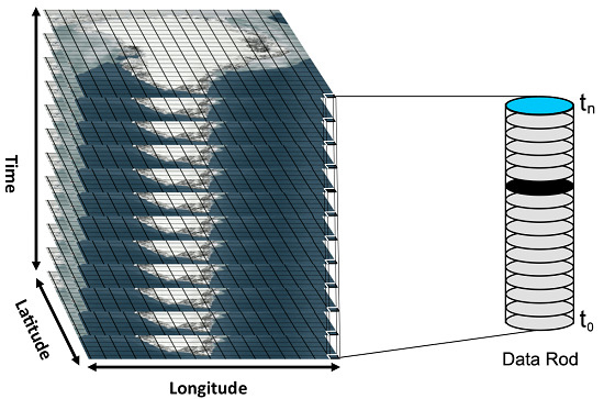
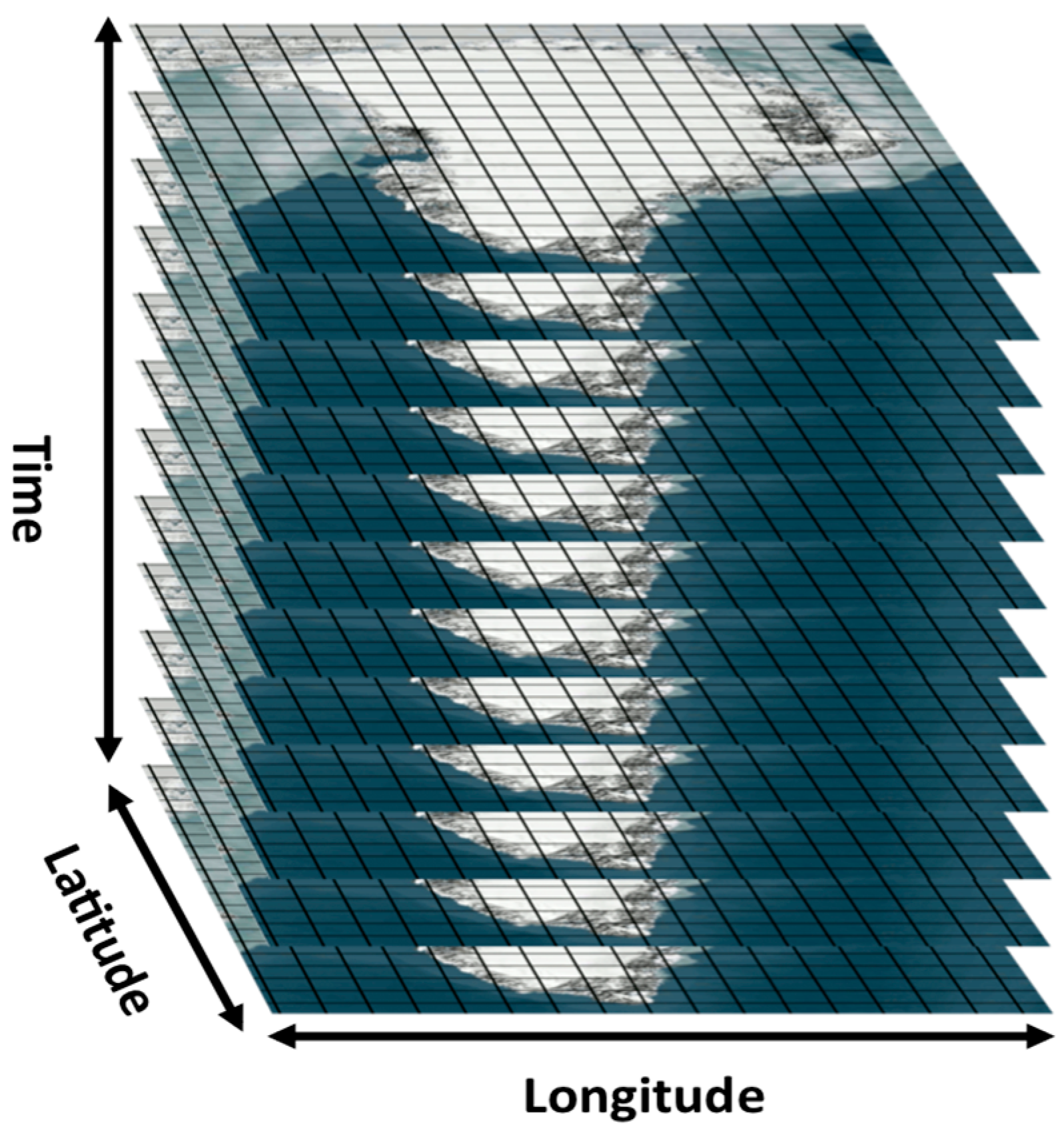
Figure 1. Stacked grids of imagery that form the basis of the three-dimensional Data Rods database structure. Within the database, pixels are stored in temporal order (vertically) at each grid cell rather than spatially (horizontal). A vertical column of pixels at a single grid cell makes up one data rod.

Figure 1. Stacked grids of imagery that form the basis of the three-dimensional Data Rods database structure. Within the database, pixels are stored in temporal order (vertically) at each grid cell rather than spatially (horizontal). A vertical column of pixels at a single grid cell makes up one data rod.

The source dataset of Greenland satellite imagery was retrieved across the Internet in the traditional “search, order, and download” manner, via FTP as either binary (flat) images for single dates and times, or as NetCDF files. A collection of Java programs and shell scripts was used to reformat the data and insert the pixels into the pure-object databases. Initial attempts to store the entire dataset in a single database were successful; however, for parallel processing and administrative tasks, we found it more efficient to break it into multiple databases, each covering a 5-year time span and containing no more than approximately 500 million pixel objects. To accelerate retrieval rates for time-series analyses, pixels were ingested into the databases in chronological order at each gridded location. This arrangement can be viewed as a vertical stack of pixels through time (the Z axis), with latitude and longitude as the X and Y axes, as shown in Figure 1. The chronological structure also facilitated the creation of the data rod objects described in the next paragraph. B-tree indexing further accelerated retrieval times for the most commonly used member data within the pixel objects. In addition, each pixel contained a reference to its source satellite, sensor, time of data collection, and geographical location, all of which were stored as objects in the databases. Figure 2 shows the object schema as a Unified Modeling Language (UML) diagram. Any of the member data contained in any object could be used as a search term. For instance, a researcher could ask to find “all the pixels in the month of June west of 45 degrees longitude where the surface temperature was greater than 0 °C” and receive a collection of pixels that matched that criteria.

Figure 2. A Unified Modeling Language (UML) block diagram of the object-oriented schema for the databases and programming architecture.

Figure 2. A Unified Modeling Language (UML) block diagram of the object-oriented schema for the databases and programming architecture.

Returning to the data rods concept, any vertical (temporal) column of pixels at one location could also be bundled into a single data rod object. Queries for time-series data at a single location, transect line, or polygon then returned all the data rods that matched the location specifications. Basic statistical methods were included with the data rod object class definitions, enabling time-series analyses at each location by simply asking the data rod to analyze itself. For example, we could query for the data rod closest to any geographical location; once retrieved, the data rod could be asked to filter itself using any time or threshold value criterion, and return the time-series mean, median, variance, or linear regression of the data values contained in its pixel objects. Additional statistical, mathematical, and filtering functions could be added to the data rod class definition as needed, expanding the potential types of analyses it could address. The individual pixel objects contained in a data rod were also independently addressable, if necessary. If multiple data rods were retrieved for the same geographical location, each covering a different 5-year period, they could be combined and analyzed as a single, comprehensive data rod object. This is the technique we used to incrementally analyze every gridded location on the Greenland Ice Sheet over the 25-year dataset.

All databases were hosted on a single 12-core server using a RAID-10 array. A total of seven databases were used, six containing the AVHRR data and one containing the LOCI mask. Parallel queries across all the databases were performed simultaneously using multicore processing; beyond 6–8 cores, however, we reached a point of diminishing returns: the primary bottleneck to retrieving the data was the speed of the disk array.

4. Analysis

To demonstrate the capabilities of the database system, we needed to illustrate how a time-centric analysis could be computed over a large spatial area against a massive remotely-sensed dataset. The task we chose was an analysis of the long-term changes in the GrIS albedo. The GrIS has been heavily studied, however most previous studies have generally limited their spatiotemporal scope to either relatively short time spans, coarse spatial or temporal resolutions, or else concentrated on small, dynamic areas. The studies that have evaluated the entirety of GrIS over long time periods, often to determine the extent of seasonal melting, typically use coarse resolution passive microwave data; e.g., [20] and [21]. The few studies that have examined the GrIS albedo at higher resolutions used shorter time spans or large temporal increments [22,23,24]. MODIS observations, with a 14-year dataset span, have informed some higher-resolution GrIS studies: Box et al. [25,26] have shown there was a 2011 albedo anomaly for the months of June through August in relation to the 2000–2008 period, and described decadal-scale downward albedo trends when using both MODIS satellite imagery and GC-Net ground data. Few studies have evaluated changes over the entire GrIS at maximal temporal and spatial resolutions. The premise of our analysis was that these limitations may be obscuring larger patterns or changes occurring on the ice sheet.

4.1. Quality Assurance

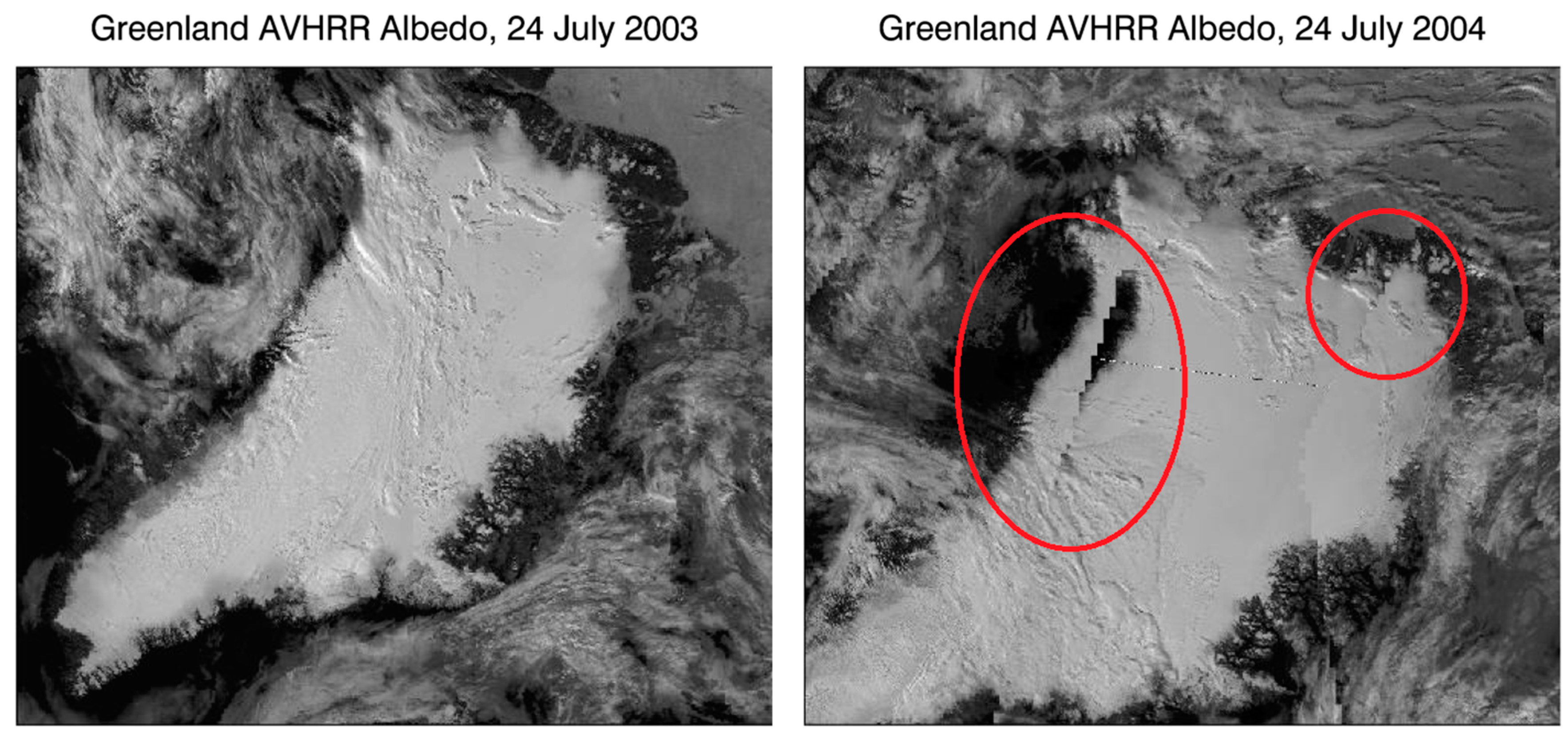
As our analysis began, we retrieved individual data rods, pixels, and full daily images from the databases to evaluate the performance of the system. Immediately, images were discovered where the swath compositing (where several satellite passes are combined to form a single image) had failed, causing severe geocoding errors; Figure 3, for example, compares a properly geocoded image with a poorly composited one. This bad data did not appear in the Completeness Report, and was apparently undiscovered until now. These images, plus others where the quantity of missing data was significant, were eliminated from this study. No longer trusting that the dataset was entirely high quality, we queried the database for all daily images from the summer months throughout the entire 25-year time span, and used the images to create animations for each year. The animations allowed us to visualize the dataset through time, detecting dates of bad compositing, and eliminating individual images where excessive noise or other errors had corrupted the data. Additional quality problems were discovered in the years 1994–1998 where changes in the CASPR processing appear to have offset geocoding by 2–4 pixels (10–20 km on the ground). In the animations, the island could be seen jittering slightly depending on the CASPR version used.

In all, 383 days of corrupted or suspect data were eliminated from consideration. It is important to note that if only a small area of ice sheet imagery or a limited time span had been viewed, as is done in many studies, these problems might never have been discovered. In this regard, analyzing the entirety of the dataset on a day-by-day basis had already proved useful.

Figure 3. An example of significant geocoding errors. The left panel is a typical albedo image of Greenland during 2003, correctly composited and geocoded. The second panel (right) shows severe geocoding errors during mid-summer 2004, most apparent in the circled areas. Note sections of the bad image are repeated and offset, and the entire island has shifted downward in the frame. Both images were obtained from the same Advanced Very High Resolution Radiometer (AVHRR) dataset using similar geographical bounding boxes and projections, and should appear identical except for natural variations in clouds and ice.

Figure 3. An example of significant geocoding errors. The left panel is a typical albedo image of Greenland during 2003, correctly composited and geocoded. The second panel (right) shows severe geocoding errors during mid-summer 2004, most apparent in the circled areas. Note sections of the bad image are repeated and offset, and the entire island has shifted downward in the frame. Both images were obtained from the same Advanced Very High Resolution Radiometer (AVHRR) dataset using similar geographical bounding boxes and projections, and should appear identical except for natural variations in clouds and ice.

4.2. Methods

The albedo imagery dataset, now cleaned of bad data, was deemed ready for use. Prior to the creation of a web-based user interface, a simple server-side Java program was constructed to access the databases, retrieve the data, and perform the analyses. Our study iteratively processed every 25 km² Greenland grid cell in the databases, excluding those not on the ice sheet (based on the LOCI mask), for a total of 72,892 grid cells. At each location we retrieved the data rod objects containing the 25-year time-series of pixels, applied temporal filtering to bin the daily data by month, and then calculated descriptive statistics. The results for all grid cells were then assembled to create images of the GrIS depicting the spatial distributions of the albedo statistics. 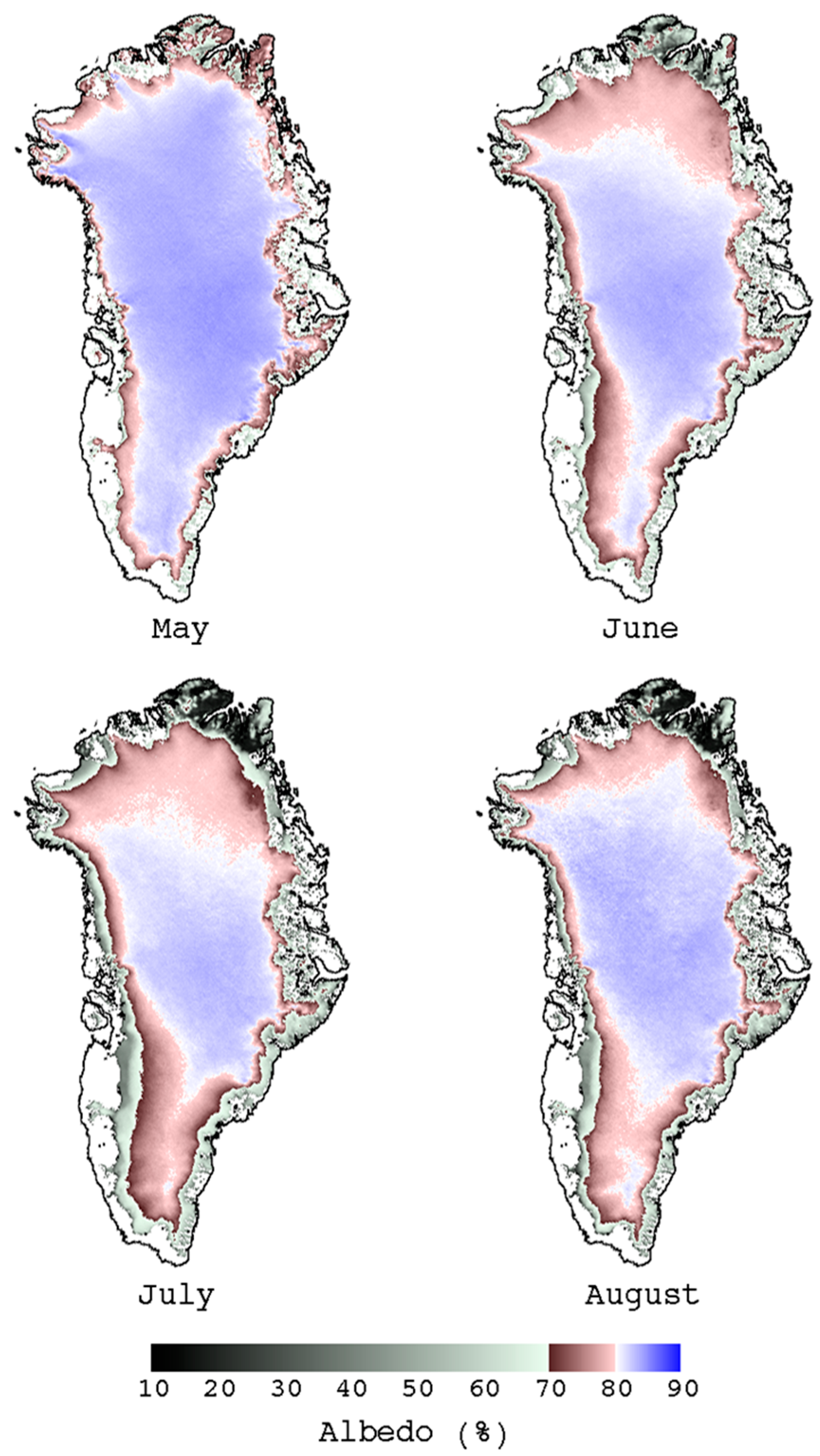For example, Figure 4 shows the median GrIS albedos for the months of May through August, summer months when the albedo can be accurately calculated and may undergo significant changes.

Figure 4. Example images produced through data rods processing. The Greenland Ice Sheet median monthly albedo is shown for the months of May through August, calculated from 25 years of albedo data, 1981 to 2005. Each grid point was temporally analyzed, and the statistical results were used to construct images of the island.

Figure 4. Example images produced through data rods processing. The Greenland Ice Sheet median monthly albedo is shown for the months of May through August, calculated from 25 years of albedo data, 1981 to 2005. Each grid point was temporally analyzed, and the statistical results were used to construct images of the island.

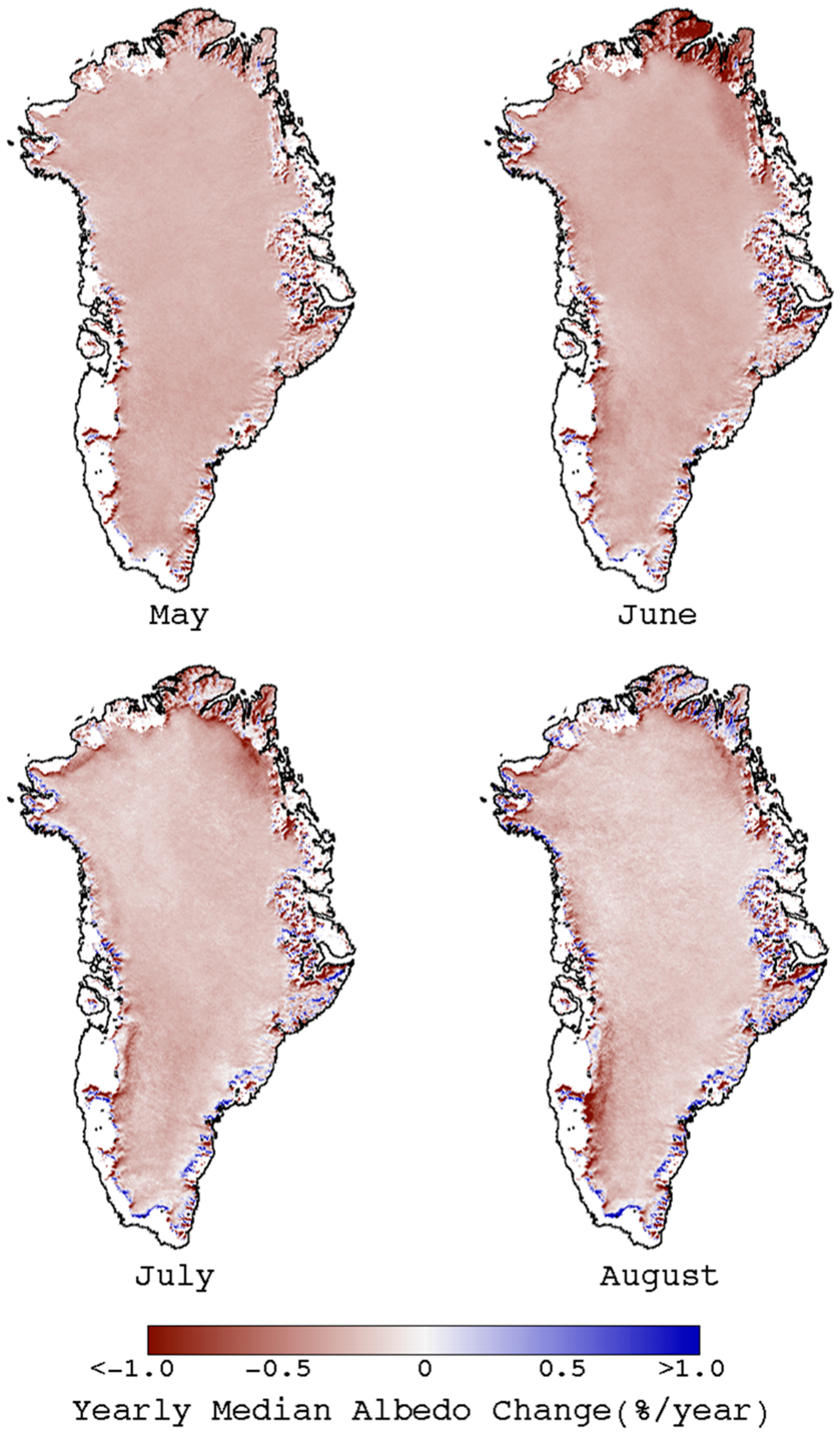
To gain a better understanding of changes in the GrIS albedo over time, the data rods were then used to evaluate the albedo trends at each grid cell. Each data rod was again filtered by month, filtered to eliminate cloudy days, and asked returned a linear regression of its albedo for the 25-year period. The results were combined to construct monthly images, shown in Figure 5. This analysis showed a nearly uniform downward albedo trend across the entire island: an unrealistic result that warranted further investigation (see Section 5).

Figure 5. An example of trend analysis using the data rods concept. Shown are the average yearly changes in albedo from 1981 to 2005 using data from the AVHRR Polar Pathfinder dataset. A data rod was created at each grid cell; filtering and statistical methods within the data rod objects then binned the data by month (May, June, July, or August), eliminated cloudy data, produced a median albedo for each month-year combination, and performed linear regressions across all years. The resulting trends at each grid cell were then used to generate the Greenland images below. Note that the 1981–2005 trend is predominantly negative for most interior locations. The magnitude of this trend was unexpected because, in general, significant interior albedo changes have been observed only after 2005 [24].

Figure 5. An example of trend analysis using the data rods concept. Shown are the average yearly changes in albedo from 1981 to 2005 using data from the AVHRR Polar Pathfinder dataset. A data rod was created at each grid cell; filtering and statistical methods within the data rod objects then binned the data by month (May, June, July, or August), eliminated cloudy data, produced a median albedo for each month-year combination, and performed linear regressions across all years. The resulting trends at each grid cell were then used to generate the Greenland images below. Note that the 1981–2005 trend is predominantly negative for most interior locations. The magnitude of this trend was unexpected because, in general, significant interior albedo changes have been observed only after 2005 [24].

All of the data retrieval and processing occurred solely on the server side; the only downloads were the final images and statistical results. Because the statistical and temporal filtering functions were already built into the data rod object class definition, the temporal processing was both flexible and easy. Standard image processing techniques could have duplicated these results, however the user would be required to download and subset large quantities of APP data, and then process it locally; performing such a one-time analysis tasks can take weeks or months, depending on the amount of coding and data reformatting necessary. The advantage here is that, once constructed and available, the databases can be used indefinitely for rapid data exploration and analysis.

5. Results and Discussion

5.1. Analysis Results

In addition to demonstrating the capabilities of the database and data rods architecture, the analysis portion of the study sought to quantify GrIS albedo trends from 1981 to 2005. Figure 5 suggests that the median albedo of nearly the entire ice sheet is decreasing by approximately 0.2% to 0.4% per year, regardless of the location. Other studies have found similar results, however, their negative trends appear to be largely a product of significant albedo changes observed after 2005, beyond the era of our analysis [24,26]. After this discovery, the data rods and database architecture were used to perform a rapid data exploration, investigating the cause of the unexpected albedo trend.

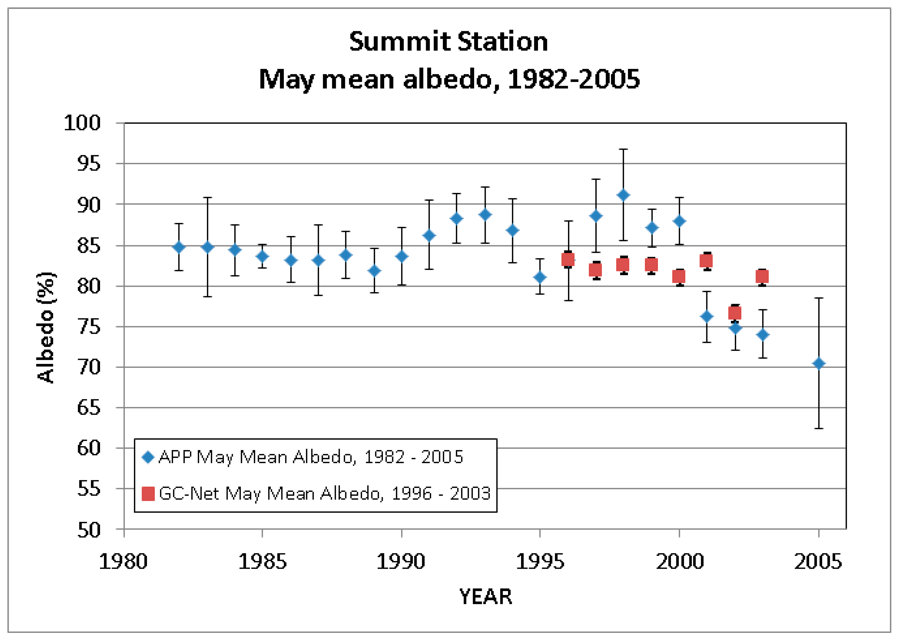
Summit Camp (72°34′46″N, 38°30′19″W) sits near the center of the island, at the apex of the ice sheet. With an average summer temperature well below freezing, melting is rarely seen. Thus, Summit Camp should have a fairly consistent albedo from year to year. Yet when we queried for a single data rod at that location and plotted the average albedo versus time (in this case, the average albedo for each month of May), a downward step function in the data was clearly visible in 2001, as shown in Figure 6. A similar 2001 downward step was present at every location on the ice sheet that we queried. The in situ GC-Net data from around the island, however, displayed no such decrease. Minor differences may be expected between the APP albedos, which cover a 25 km² ground footprint, and the GC-Net data, due to differences in their respective instrumentation, fields of view, sampling frequencies, and post processing techniques. However, a sudden, persistent offset was cause for concern. The APP dataset uses a succession of NOAA satellites and AVHRR sensors, with NOAA-16 data beginning in January of 2001; the fact that the downward albedo step occurred at the same time as a switch to a different satellite seemed to be more than a coincidence.

Each AVHRR sensor requires calibration, with the reflectance and near-IR data needing post-collection calibration because it cannot be done on-orbit. Albedo calculations are thus highly dependent on the quality of the post-collection calibration. The CASPR albedo algorithms assume the data has already been calibrated, so no additional checks were performed when the APP dataset was generated. The APP documentation and literature was searched to verify that the calibrations had been properly applied, however the results were inconclusive. Subsequent discussions with knowledgeable users led us to conclude that the calibrations—and thus the albedos—were incorrect, producing a downward step at the start of NOAA-16 data.

Although we did not set out to build a system specifically designed to evaluate dataset quality, the data rods databases ultimately proved especially efficient at doing so. In all, the following errors were identified: Visible sensor calibration issues, and the resulting incorrect albedos starting in 2001; multiple months of image swath compositing errors during 2004 and 1983; entirely missing images that were not identified in the completeness report; and several days where the IR and visible sensor data in the APP dataset were inexplicably swapped. Additionally, two different versions of the CASPR software were used to create the APP data, the first through year 1998, and a second version starting in 1994 and onward. During user data downloads, it was possible for the overlapping data versions to become randomly intermixed (an error invisible to the user). Since the two software versions used different geocoding parameters and cloud masking algorithms, this caused significant inconsistencies in the long-term dataset, including the pixel jitter mentioned in Section 4.1.

Figure 6. Mean cloud-free May albedo values from the AVHRR Polar Pathfinder (APP) satellite dataset and Greenland Climate Network (GC-Net), for Summit Station, Greenland. The error bars show one standard deviation. The APP albedos are based on pixels with a 25 km² ground field of view; the GC-Net albedos were collected in situ. Missing years are due to insufficient data. Of special note is the sudden drop in APP mean albedos starting in 2001.

Figure 6. Mean cloud-free May albedo values from the AVHRR Polar Pathfinder (APP) satellite dataset and Greenland Climate Network (GC-Net), for Summit Station, Greenland. The error bars show one standard deviation. The APP albedos are based on pixels with a 25 km² ground field of view; the GC-Net albedos were collected in situ. Missing years are due to insufficient data. Of special note is the sudden drop in APP mean albedos starting in 2001.

Importantly, the APP dataset was made available to the public in 2008 and used for multiple studies since that time, yet none of the errors had been detected until now. By using the time-centric processing of data rods and the query tools of the database architecture, the errors became apparent immediately. The 2001 albedo error, for instance, while distinctive in areas with a seasonally consistent albedo, was often obscured in areas with significant seasonal variability. These same, dynamic areas are common regions of interest, and it would be easy for a narrowly-focused study to overlook the problem. In this regard we feel that the “big data” approach to our analysis, that of viewing the whole of the GrIS through time, met its objectives in that it found previously undetected information.

Following our study, the APP dataset was removed from distribution. It is currently being reprocessed using the proper sensor calibration values as well as a single, consistent software version. Researchers who cited the earlier, incorrect dataset in publications have been informed of the potential errors.

While the discovery of the errors precluded any meaningful scientific conclusions regarding the GrIS albedo, it did validate the original premise: When the dataset was viewed as a whole, in a high spatiotemporal resolution, new information was discovered that had not been seen when viewing smaller areas or limited time spans. We suggest this kind of analysis should be performed on all large spatiotemporal databases to insure their quality and consistency.

5.2. Database Performance

Any database performance metrics are, of course, highly dependent on the hardware and software configuration. Nevertheless, the metrics we give here serve to demonstrate that massive remotely-sensed datasets can be managed within a series of pure-object databases while providing an efficient method for performing time-centric data analysis. Time-centric data exploration using the combined architecture of the pure-object databases and data rod schema was rapid: A random query for a single data rod, retrieving all the pixel data at a given location through time, took 6.6 seconds (uncached) or 2.2 seconds (cached). Iteratively processing all 72,892 GrIS data rods in the databases and creating the statistical images took approximately 2 days. Critically, we iterated across the data rods in the same order in which they had been originally entered into the databases, taking full advantage of the database software’s internal caching. If, on the other hand, we had randomly accessed every grid cell or processed the data counter to its organization within the databases, processing times would have been considerably longer. Used efficiently in this manner, the databases provided a relatively quick method for data exploration and analysis without the need for downloading or local processing. In contrast, a similar analysis project that ran concurrent with ours, but employing traditional techniques of data downloading and code generation, took several weeks to complete.

Development of the initial data rods architecture also took considerable design and coding effort, of course, but the resulting databases and code structure are perpetually reusable. Once the databases are established, subsequent analyses can be completed in a fraction of the time as compared to traditional temporal analysis methods.

6. Conclusions

In our study, we developed a temporally-oriented schema for storing, filtering, and retrieving information contained in massive remotely-sensed datasets. Rather than storing imagery in a spatial orientation for single dates and times, as is typically done, we reorganized it into temporal columns, “data rods”, where each rod represents all the information available at a set of gridded coordinates through time. This concept fundamentally restructured how the data was internally represented in a computer, permitting rapid time-centric querying, thresholding, and data retrieval. The ultimate objective was to accelerate temporal analyses, creating a tool particularly useful for climatological studies.

The data, once reformatted into data rod structures, was stored in a series of pure-object databases. The advantage to this approach was that, when creating billions or trillions of database entries, using a pure-object database avoids some of the performance limitations that may occur with relational or hybrid object-relational databases. Combined with a simple user interface and server-side processing, the result was a tool that permitted extremely fast temporal analysis at any desired location. This architecture also circumvented the time-consuming process of having to search for, and then download, massive datasets, or having to create custom analysis programs.

To demonstrate the scientific potential of the data rods and database system, we analyzed 25 years of Greenland albedo imagery. The premise of our analysis was that, by viewing the Greenland ice sheet as a whole, in high temporal and spatial resolution, new information might be revealed that was missed by previous studies. Instead, the analysis found a series of significant errors in the original dataset that had gone undetected. The databases and data rods system were then used to determine the cause of the errors, which were shown to have occurred during the original generation of the albedo imagery, prior to 2008.

The data rods system was crucial to finding and identifying the errors in the Greenland dataset. While we could not make any scientific conclusions regarding changes in the ice sheet’s albedo, our analysis served to demonstrate another capability of the data rods system: quality assurance. By temporally reorienting the dataset and providing fast analysis tools, the system rapidly identified dataset errors that occurred through time.