1. Introduction
The southwest coastal plains in Taiwan are highly developed areas of economy and agriculture. As production continues to increase, the supply of surface water gradually falls short of demand, causing industries to turn to low-cost groundwater as the substitute; however, excessive pumping of groundwater often results in land subsidence [
1,
2,
3]. Ching
et al. [
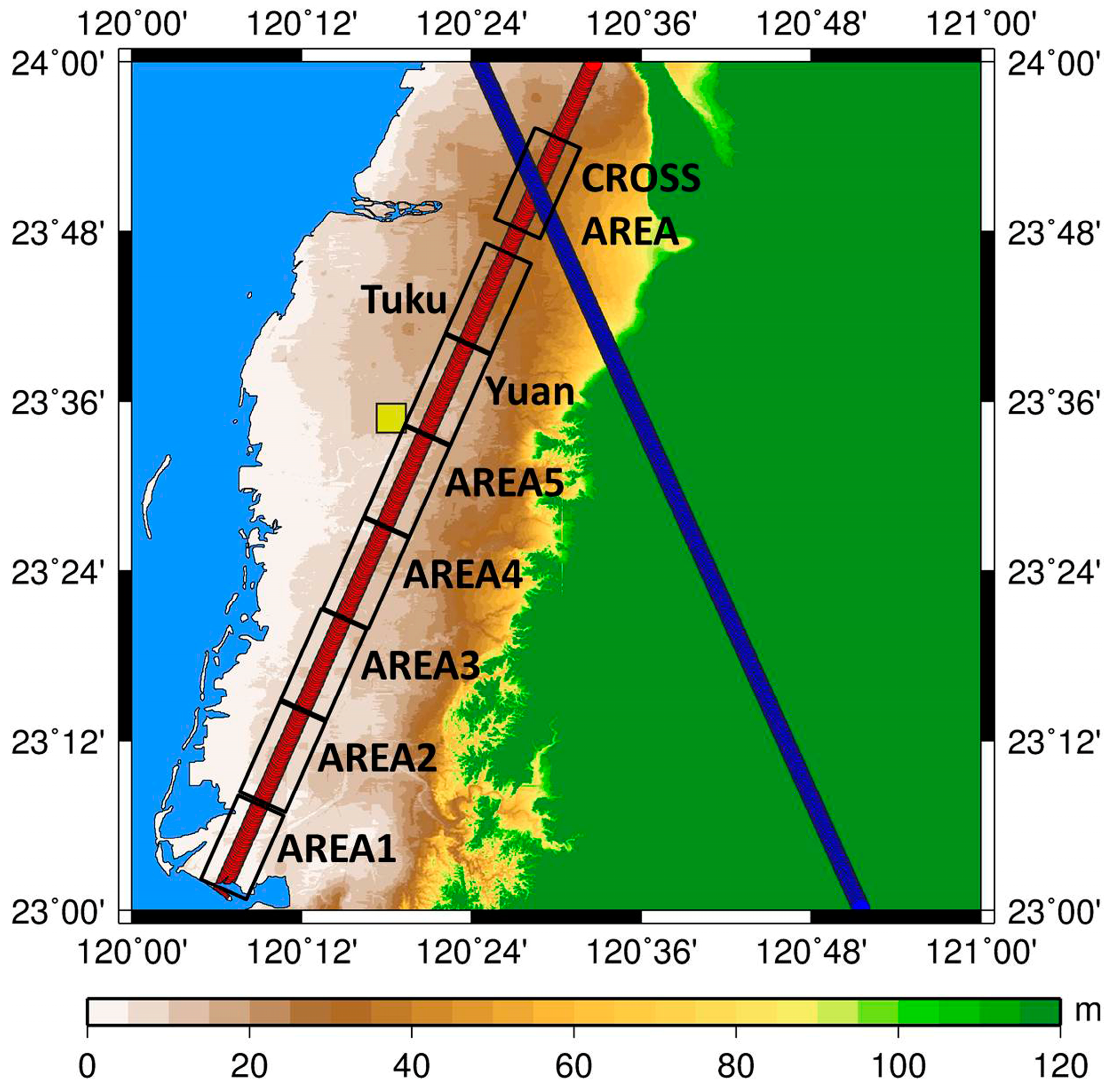
4] combined Global Positioning System (GPS) data with geodetic precise leveling data to estimate land surface vertical motion rates in Taiwan. They found that land subsidence mostly occurred in coastal regions and in Tuku and Yuanchang of Yunlin County. Coastal land subsidence results in the irreversible submergence of coastal inland and, therefore, saltwater intrusion into surface and ground waters, soil salinization, and other disastrous consequences, such as ecosystem changes and socioeconomic impacts [
5]. The Taiwan High-Speed Rail passes through Yunlin County, where land continuously subsides, and safety issues for trains that operate at high speeds create serious concerns. Accordingly, the accurate monitoring of land subsidence in Taiwan remains an important and immediate task to prevent disasters.
Vertical land motions have traditionally been monitored using geodetic precise leveling and Global Navigation Satellite System (GNSS)/GPS data [
4,
6]. Geodetic leveling has the advantage of providing land orthometric heights with high accuracy to derive vertical motion rates. However, the field work involved in leveling survey is labor intensive, time consuming, and expensive. Completing a loop of leveling survey takes time, causing discontinuity of measurements in time. As a recent advancement in space geodetic technique, GNSS can quickly obtain long-term continuous 3D coordinates to derive vertical motion rates. However, coordinate accuracy in the vertical component is not as precise as that in the horizontal one. Setting up densely distributed GNSS stations in remote areas also requires manpower, thereby complicating the implementation. Even if GNSS permanent stations are built, the rates of vertical motions can only be determined after years of data collection. Interferometry Synthetic Aperture Radar (InSAR) is another alternative technology widely used to monitor regional vertical motions [
2]. Nevertheless, this technique is inadequate for analyzing the rate changes and the trends of vertical motions because discontinuous InSAR measurements only cover a short time span and land motions contain seasonal and long-term signals.
Satellite altimetry is a developed oceanographic technology used to synoptically map global ocean surfaces and sea level changes with unprecedented accuracy and resolution. The basic observational principle is to measure ranges from a satellite to ocean surfaces by transmitting an electromagnetic radar pulse to measure its round-trip travel time between the receiving antenna of the satellite and the instantaneous ocean surface. In practice, the observed measurement in satellite radar altimetry is a time series of the received power distributions of the reflected pulses; it is often referred to as the altimeter waveform and generally fulfills all assumptions mentioned by Brown [
7] for calculating the range,
R =
c × Δ
t/2 (where Δ
t is the travel time and
c is the speed of light)
. Satellite altimetry can provide long-term and repeated measurements nearly globally and can operate under different weather conditions. Therefore, it may potentially be applied to monitoring land surface changes. However, altimetry was originally designed for open oceans, and so latent problems must be addressed before it can be implemented over non-ocean surfaces. Altimetric waveforms reflected from non-ocean surfaces such as rivers, small lakes, and lands covered with vegetation or buildings are quite complex or noisy, and indicate non-conformance to the typical Brown model [
7], which was originally designed for deep-ocean altimetry sea surface height (SSH) retrieval. As a result, inaccurate ranges between the satellite and the reflected surface are derived from the default gates based on the Brown model; for example, default gate 24.5 in a 64-sample waveform for Topex/Poseidon (T/P) and 32 in a 104-sample waveform for Jason-2 (J-2). In this regard, waveform retracking technique was developed to calculate range correction using the gate difference between the default and retracked gates and thus to improve the accuracy of altimetry over land surfaces.
Many useful retrackers have been developed to improve altimetry measurements in different reflected surfaces, including NASA V4 (β-) retracker [
8], offset center of gravity retracker [
9], traditional [
10] and modified threshold retracker (MTR) [
11], ocean and ice retrackers [
12], and subwaveform threshold retracker (STR) [
13]. Previous studies have applied retracked altimetry to monitor water level changes in inland rivers [
14,
15,
16], lakes, reservoirs [
17,
18,
19,
20], and vegetated wetlands [
21], as well as to track Antarctic elevation changes [
22]. The accuracy of the retrieved surface heights varies by the study area. Only a few researchers have employed retracked altimetry data to monitor solid earth deformation. For example, Lee
et al. [
11] estimated Laurentia crustal motion observed using retracked T/P altimetry with an average uncertainty of 2.9 mm/yr, which is comparable to the 2.1 mm/yr uncertainty of recent GPS solutions. In accordance with their idea, the MTR is excellent for solving the bump in the pre-leading edge of land reflected waveforms. Yang
et al. [
13] proposed the use of STR for ERS-1 altimetry to measure SSHs in the Antarctic Ocean and improved the SSH precision ranging from 0.2410.193 m compared with the tide gage records at Port Station. Although STR was only employed in ice-covered oceans, it can also be used on lands because this retracker uses a part of the full waveform that does not contain the pre-leading edge bump for threshold retracking [
13]. Therefore, both MTR and STR can improve the accuracy of altimetric surface heights by reducing the containment of the pre-leading edge bumps [
11,
13] and were used in this study.
Instrument error, medium error, including ionosphere delay and wet/dry troposphere delay, and specific geophysical corrections should be considered in altimetric measurements [
23]. Over ocean, wet troposphere delay is calculated by means of water vapors observed by microwave radiometers onboard altimeter satellites, but these are unable to work over land [
24,
25]. Considering this limitation, most previous studies corrected altimeter data by using wet troposphere delay derived from global climate models (e.g., [
26]); however, the accuracy of these models is unknown or varies across regions on lands. Therefore, further assessing the accuracy of the correction derived from global climate models is needed. In recent years, GNSS was increasingly used to estimate regional wet troposphere delay [
27,
28], which can serve as basis to assess the delay derived from global climate models and improve altimetric measurements over land. Fernandes
et al. [
29] reported that the means of differences between the zenith wet delays derived from GNSS and microwave radiometers onboard altimeters range between −11 mm to −5 mm with standard deviations (STDs) in the range of 17–22 mm.
Southwestern Taiwan is undergoing serious land subsidence where satellite altimetry ground tracks repeatedly pass, and well-established GNSS tracking stations are located in this area. In this study, we therefore reprocessed altimetry waveforms, including T/P and J-2, by using waveform retracking algorithms to improve the accuracy of land surface heights (LSHs) and vertical land motion trends. The wet troposphere delay estimated from continuous GNSS tracking data was also compared with that derived from the global climate model to evaluate the impact of this delay on the accuracy of estimated vertical motion rates.
3. Data
The design of the Jason-1 (J-1) satellite instrument and problems in data processing hindered the completion of terrestrial data aside from poor accuracy [
14]; therefore, J-1 data were neither sufficient nor appropriate for this study. Only pass 51 and pass 164 of T/P and J-2 altimetry passing over Southwestern Taiwan were thus used. T/P data including 10 Hz 64-sample waveforms, which correspond to an along-track sampling of ~660 m, were acquired from Geophysical Data Records (GDRs) and Sensor Data Records (SDRs). The acquired T/P data cover the period from December 1992 to August 2002 (cycles 10–364). J-2 data, including 20 Hz 104-sample waveforms (along-track space is ~330 m), were obtained from product version “D” Sensor Geophysical Data Records (SGDRs), covering the period from August 2008 to January 2014 (cycles 4–205). Both data have the same repeat cycle of 10 days and were provided by PODAAC, JPL under a contract from NASA. All acquired terrestrial altimetry data were corrected through corrections in the instrument, medium (ionosphere corrections based on onboard DORIS for T/P and Global Ionosphere Maps for J-2; wet and dry troposphere corrections based on the European Center for Medium-Range Weather Forecasts (ECMWF)), geophysical parameters (solid tide described in Cartwright and Edden [
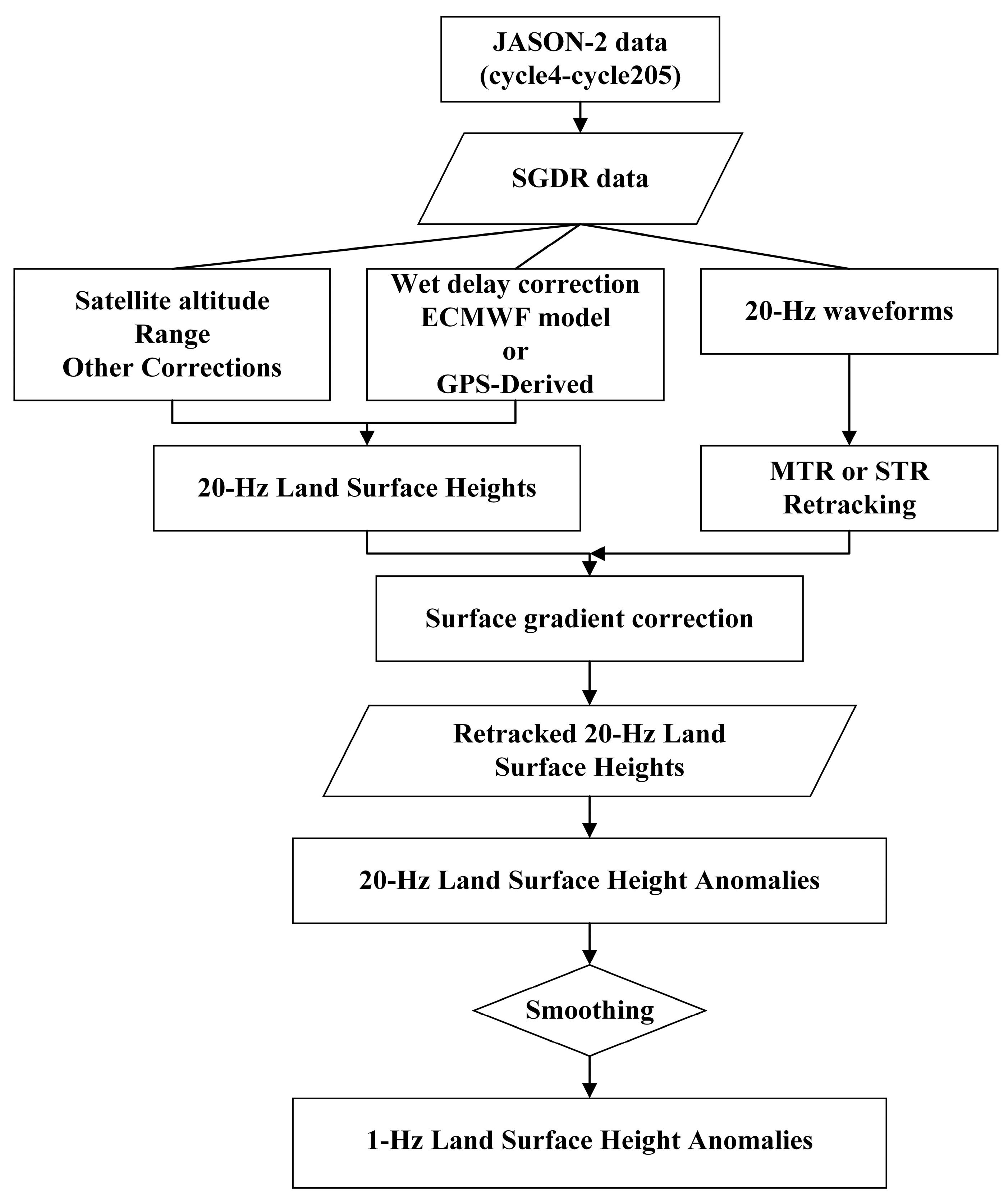
30] and pole tide described in Wahr [
31]), waveform retracking, and terrain gradient.
GNSS data with a sampling rate of 30 s were obtained from the Beigang GNSS permanent tracking station (latitude: 120°18′19′′; longitude: 23°34′47′′; ellipsoid height: 42.729 m; orthometric height: 22.875 m). The GNSS data, which cover the period of 1995–2002 and 2008–2011, were provided by the Satellite Survey Center of the Department of Land Administration, Ministry of Interior, in Taiwan and were used to derive wet troposphere delay.
A Taiwan digital elevation model (DEM) with a 3′′ × 3′′ spatial resolution [
32] was introduced to correct the terrain gradient. The LSH from altimetry refers to the T/P ellipsoid, and DEM is in an orthometric height system. Thus, Earth Gravitational Model 1996 (EGM96) was used to transform DEM orthometric heights into ellipsoid heights in this study. In addition, a constant of 0.7 m was implemented to correct the different semi-major axes of the T/P and WGS84 ellipsoids [
11].
4. Methodology
The acquired T/P and J-2 altimeter data contain satellite altitude, the range between the altimeter and the reflected surface, echoed waveforms, and related errors or geophysical corrections. The wet troposphere delay was estimated over land with the use of a global atmosphere model, ECMWF. To evaluate the estimated delay from ECMWF, wet troposphere delay was also calculated with GNSS tracking measurements by means of the precise point positioning (PPP) technique. The basic concept is calculating the amount of residual delays by using the random walk model on the basis of an initial value derived from a meteorological model [
33]. The delay can be estimated using the PPP in four steps. First is acquiring the observations of the GNSS tracking stations, including dual-frequency code and carrier phase measurements. Second is acquiring the precise ephemerides and clock corrections provided by the International GNSS Service. Third is processing the zero-differenced dual-frequency code and carrier phase measurements. The calculation should include all items of error corrections, troposphere delay estimation, and ionosphere-free combination. Fourth and last is estimating the unknown parameters, including the 3D coordinates of the receiver, receiver clock error, and wet troposphere delay.
GNSS-Inferred Positioning System and Orbit Analysis Simulation Software (GIPSY-OASIS), developed by the Jet Propulsion Laboratory (JPL) and maintained by the Near Earth Tracking Applications and Systems groups, was used in the study [
34]. The orbit product used is JPL GIPSY final orbits and satellite clock offsets. The 3-D root mean square (RMS) accuracy of the orbit is 2.5 cm and the latency is <14 days. A standard hydrostatic priori formula, which is equal to 1.013 × 2.27
e−0.00011h (where
h is ellipsoid height of the station in meter), was introduced as a priori dry zenith delay and the value of zenith wet delay was set as 0.1 m. Tregoning
et al. [
35] indicated that a priori zenith hydrostatic delay error generated errors in zenith delay estimates of up to 5 mm and seasonal variations of up to 1 mm amplitude using GPS data analyzed using a double-difference approach. Global Mapping Function, which can be implemented easily, perform better than Niell Mapping Function, and provide smaller station height biases compared with an expansion of the Vienna Mapping Function [
36], was used in the study. The satellite elevation cut-off angle was set to 10°. Finally, the troposphere gradient parameters as a Random Walk wet delay were solved as well [
37].
Applying satellite altimetry over land is more difficult than studying the ocean because the accuracy of LSH is relatively low since the returned waveforms are complicated as a result of the reflected surface covered by vegetation, buildings, and other structures located on it.
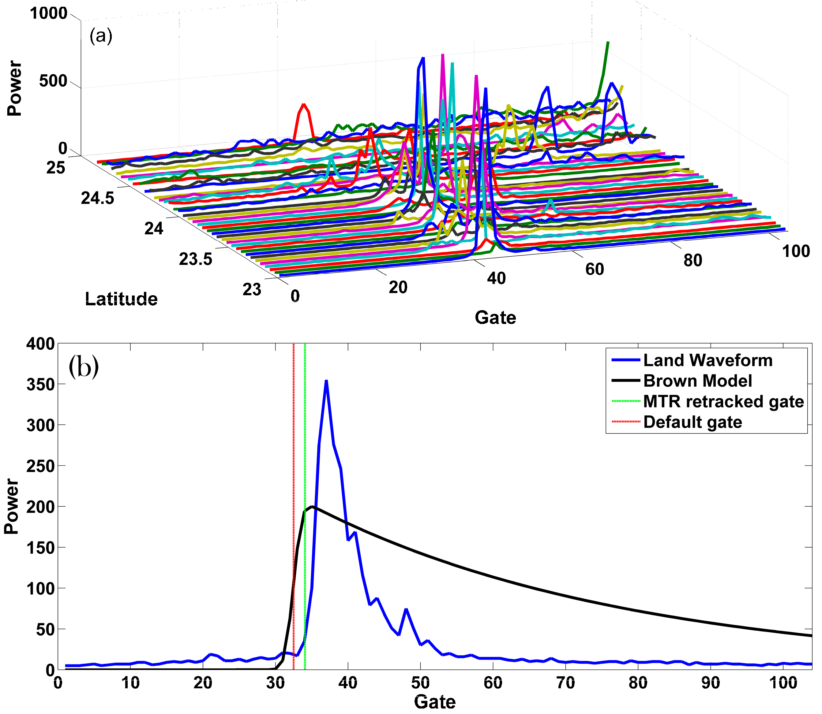
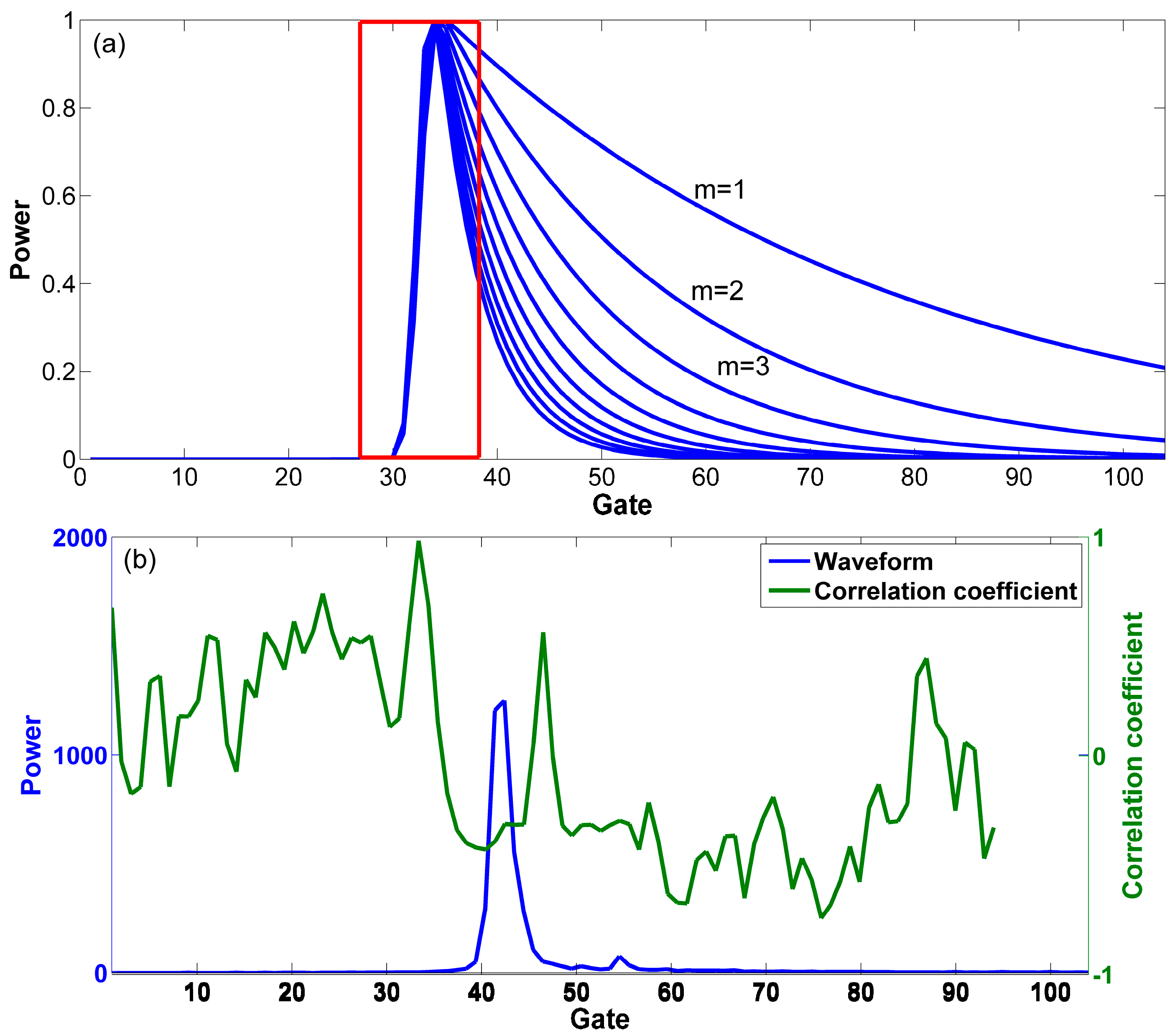
Figure 2a shows that J-2 along-track waveforms are highly complex and completely different from the default Brown model. A bump, which degrades accuracy, also exists in the pre-leading edge of most waveforms.
Figure 2b shows that a significant bias exists between the default and retracked gates. This bias indicates that the altimeter range derived from the default gate is entirely incorrect. To address this issue, waveform retracking should be applied to process complex waveforms and thus improve the accuracy of LSH. The retracked range correction can be expressed as
where
Rg is the retracked gate,
Tg is the default tracking gate of ocean waveform, and Δ
d = τ ×
c/2 (τ = 3.125
nanosecond).
In this study, MTR [
11] and an improved STR [
13] that both function to remove the effect of the pre-leading edge bump were applied to calculate the range corrections for the LSH derived by the default gate.
Originating from the traditional threshold retracker (TR) [
10], MTR was developed by Lee
et al. [
11], who reported that an average uncertainty of Laurentia crustal motion using T/P retracked by MTR is 2.9 mm/yr, which is close to the 2.1 mm/yr of recent GNSS solutions. MTR is capable of solving two problems as a result of complex land waveforms retracked by TR. First, only several preceding gates (for example, gates 5–7) in the pre-leading edge are averaged as the standard to calculate thermal noise; however, bumps occur in the pre-leading edge of complex land waveforms, causing misestimated thermal noise. Second, the maximum power of ocean waveform is generally at the apex of the leading edge, but this case is not always true for land waveforms. Thus, the retracked gate by TR could be incorrect. MTR is obviously distinct from the traditional TR in calculating thermal noise and identifying the maximum power of the leading edge by calculating two types of waveform differences, namely,
Difference I and
Difference II. The formulas are as follows:
where
P(i) is the power of the
ith gate,
i = 1–64 for T/P and 1–104 for J-2.
The thermal noise level and the maximum power of the leading edge can be determined in three steps. The first is searching from the first
Difference I; the gate of the thermal noise level is obtained when positive
Difference I becomes negative. The second is searching for a gate where the maximum of
Difference II is located and then continuing to find the next gate whose
Difference II becomes negative, which is called the
nth gate. If
Difference I(
n) is negative, the maximum power of the leading edge can be found in the
nth gate; otherwise, it can be found in the (
n + 1)th gate. The third step is retracking waveform with the traditional 10% TR using the calculated thermal noise level and the maximum power of the leading edge. The threshold value of 10% was suggested by Lee
et al. [
11] and Cheng
et al. [
38] for monitoring vertical land deformation.
Figure 2.
(a) J-2 along-track waveforms on land; (b) The MTR retracked gate (green dashed line) and the default gate (red dashed line) of the leading edge in J-2 land waveform. The blue and black curves are land waveform and Brown model, respectively.
Figure 2.
(a) J-2 along-track waveforms on land; (b) The MTR retracked gate (green dashed line) and the default gate (red dashed line) of the leading edge in J-2 land waveform. The blue and black curves are land waveform and Brown model, respectively.
Yang
et al. [
13] proposed STR based on correlation analysis by using the Brown model as a reference waveform. This retracker has been successfully applied to compute SSHs in the Antarctic Ocean with the advanced SSH precision from 0.241–0.193 m compared with the Port Station tide gage records. The advantage of STR is that only a part of the entire waveform is used to avoid the bump in the pre-leading edge involved in waveform retracking. Since the reflected radar signals from land are mostly specular (or quasi-specular) waveforms and the widths of land-reflected waveforms vary with land covers, in the present study we used the Brown model with an additional parameter that controls the descending slope of the waveform to establish a reference waveform. The returned power of land waveform can be expressed as
where
A is the amplitude of the power,
erf is the Gaussian error function, σ is a parameter associated with the slope of the leading edge governed by significant wave heights,
t is the time of the gate, τ is the midpoint of the leading edge, α is an exponential decay parameter in the trailing edge and is regarded as a constant of 137, and
m is an additional parameter to control the width of the specular waveform.
To apply STR, multiple standard reference waveforms were established using different
m values and then the leading edge of the reference waveforms including gates 24–34 (in total 11 gates) was extracted, which are called reference subwaveforms (
Figure 3a).
m = 1 represents the traditional Brown ocean model. The reference subwaveforms were then sequentially compared with a part of the entire altimetric land-echoed waveform that contains 11 gates in order (e.g., gates 1–11, gates 2–12, gates 3–13,
etc.) to calculate the correlation coefficients. The altimetric subwaveform with the largest positive coefficient compared with the reference subwaveforms represents the true leading edge (
Figure 3b). This subwaveform was later used for waveform retracking by 10% TR to retrieve the accurate retracked gate in accordance with Lee
et al. [
11] and Cheng
et al. [
38].
Figure 3.
(a) Reference waveforms derived from different m values. The red box contains the reference subwaveforms of the leading edges; (b) Correlation coefficients of the J-2 waveform and the reference subwaveform derived by Equation (4) with m = 80 (Blue curve is J-2 waveform, and green curve is correlation coefficients).
The actual orbits of T/P and J-2 altimeters shift in the cross-track direction of ±1 km. In the along-track direction, the mean distance between consecutive 1 Hz measurements is about 6 km. Thus, with respect to along-track reference points, the measurements acquired during the various 10-day cycles are non-repeated exact observation points, displaced by ±1 km in the across-track direction and ±3 km in the along-track direction. To adjust the measurements of the actual ground track to the nominal ground track, a Taiwan DEM introduced in
Section 3 was used to correct the terrain gradient with bilinear interpolation. The formula is expressed as [
11]
where
LSHnom is the LSH after terrain gradient correction,
LSHcyc is the LSH before terrain gradient correction,
DEMnom is the DEM at points of the nominal ground track, and
DEMcyc is the DEM at the points of the actual ground track.
Afterwards, the land surface anomaly (LSA) can be derived by subtracting the corresponding DEM from the corrected LSH. To eliminate or reduce LSA noises, spatial and temporal smoothing was applied to T/P 10 Hz and J-2 20 Hz LSA. For spatial smoothing, T/P 10 Hz and J-2 20 Hz LSA were averaged to 1 Hz LSA by a simple average individually after removing the outlier. The outlier was defined as the difference between T/P 10 Hz (or J-2 20 Hz) and 1 Hz LSAs that is larger than three times of the STD of 1 Hz averaged LSAs. A boxcar filer with a width of nine cycles was used for temporal smoothing.
Figure 4 shows the complete retracking procedure for the J-2 altimetry data used in this study. The same one was applied to T/P data. Finally, two 1-Hz LSAs were averaged in each study area, corresponding to the along-track space of 12 km, to estimate the rates of land vertical motions, which were compared with independent observations.
Figure 4.
Flowchart of retrieving J-2 LSA by waveform retracking.
Figure 4.
Flowchart of retrieving J-2 LSA by waveform retracking.
5. Results and Discussion
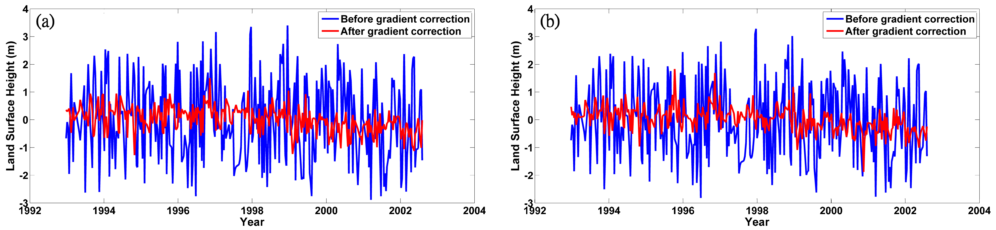
An example of terrain gradient correction is demonstrated in
Figure 5, illustrating the variation in the retracked LSH (a mean is removed) with the terrain gradient correction significantly decreased as the STDs reduced from 1.47–0.47 m in Tuku and from 1.37–0.44 m in Yuanchang; therefore, terrain gradient correction is effectively helpful and meaningful in improving the accuracy of retracked altimetric LSH averaged over a specific area. In this study, the PPP technique of GIPSY-OASIS was used to determine wet troposphere delay by estimating an unknown parameter [
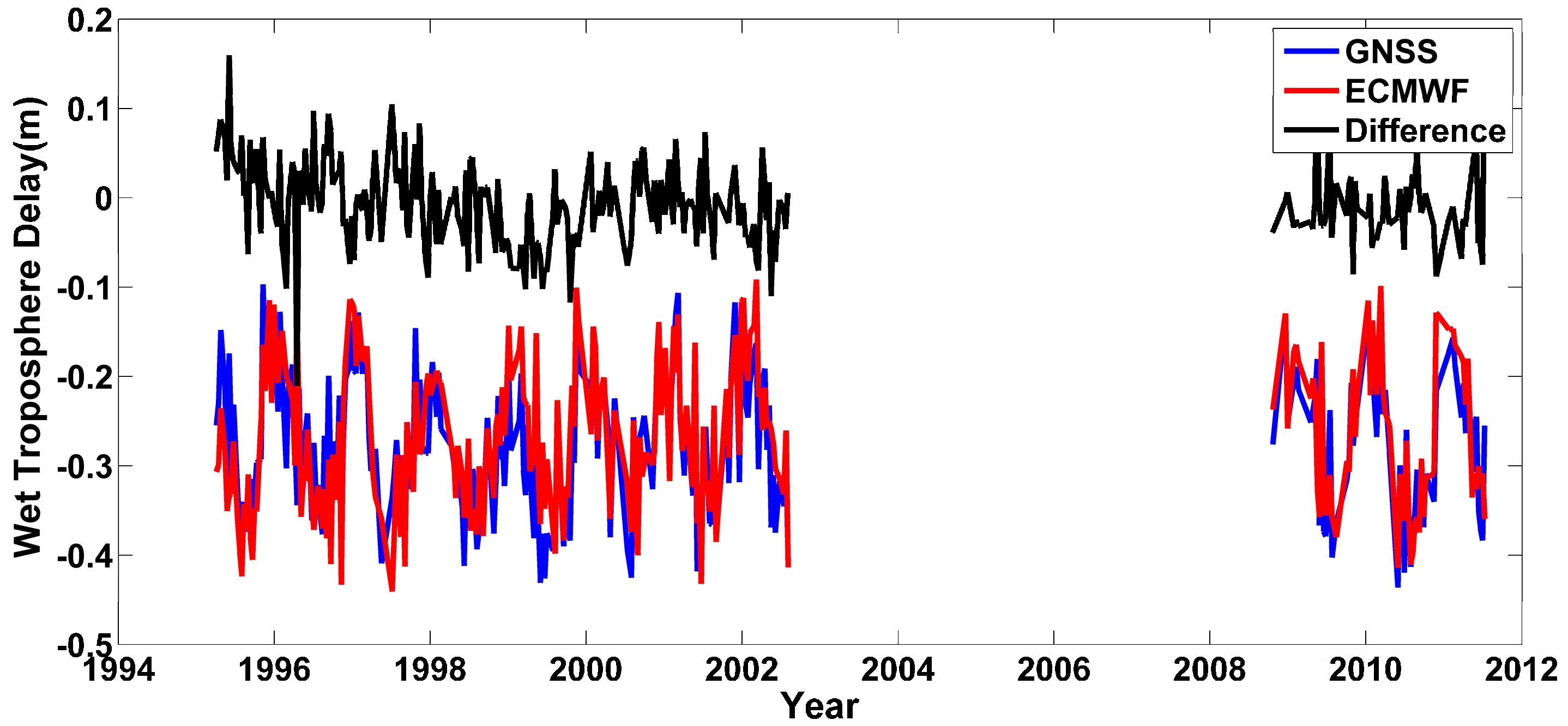
34], which can be adopted to correct altimetric data instead of the one derived from the ECMWF model. The wet troposphere delays derived from GNSS and ECMWF agree well (
Figure 6) with a correlation coefficient of 0.82, and the mean difference is −0.80 cm (STD = 4.73 cm). The means of differences in the periods of the T/P and J2 missions are −0.69 cm (STD = 4.89 cm) and −1.01 cm (STD = 4.21 cm), and correlation coefficients are 0.81 and 0.87, respectively, indicating both agree slightly better in the T/P covering period. Fernandes
et al. [
25] reported that ECMWF-derived dry and wet troposphere corrections are commonly referred to the model orography or sea surface rather than actual surface, causing the errors of 2.5 cm per each 100 m for dry correction and of 5% for wet correction due to the height error of 100 m. Therefore, in our study the error of ECMWF-derived wet troposphere delay resulting from not considering the GNSS station altitude of 22.875 m, is less than 1 cm and could not significantly affect the trend rates of land motions.
Figure 5.
Comparison of the retracked altimetric LSHs with and without terrain gradient correction (a) in Tuku and (b) in Yuanchang. Means of LSHs are removed.
Figure 5.
Comparison of the retracked altimetric LSHs with and without terrain gradient correction (a) in Tuku and (b) in Yuanchang. Means of LSHs are removed.
Figure 6.
Comparison of wet troposphere delays derived from GNSS and ECMWF in Yuanchang.
Figure 6.
Comparison of wet troposphere delays derived from GNSS and ECMWF in Yuanchang.
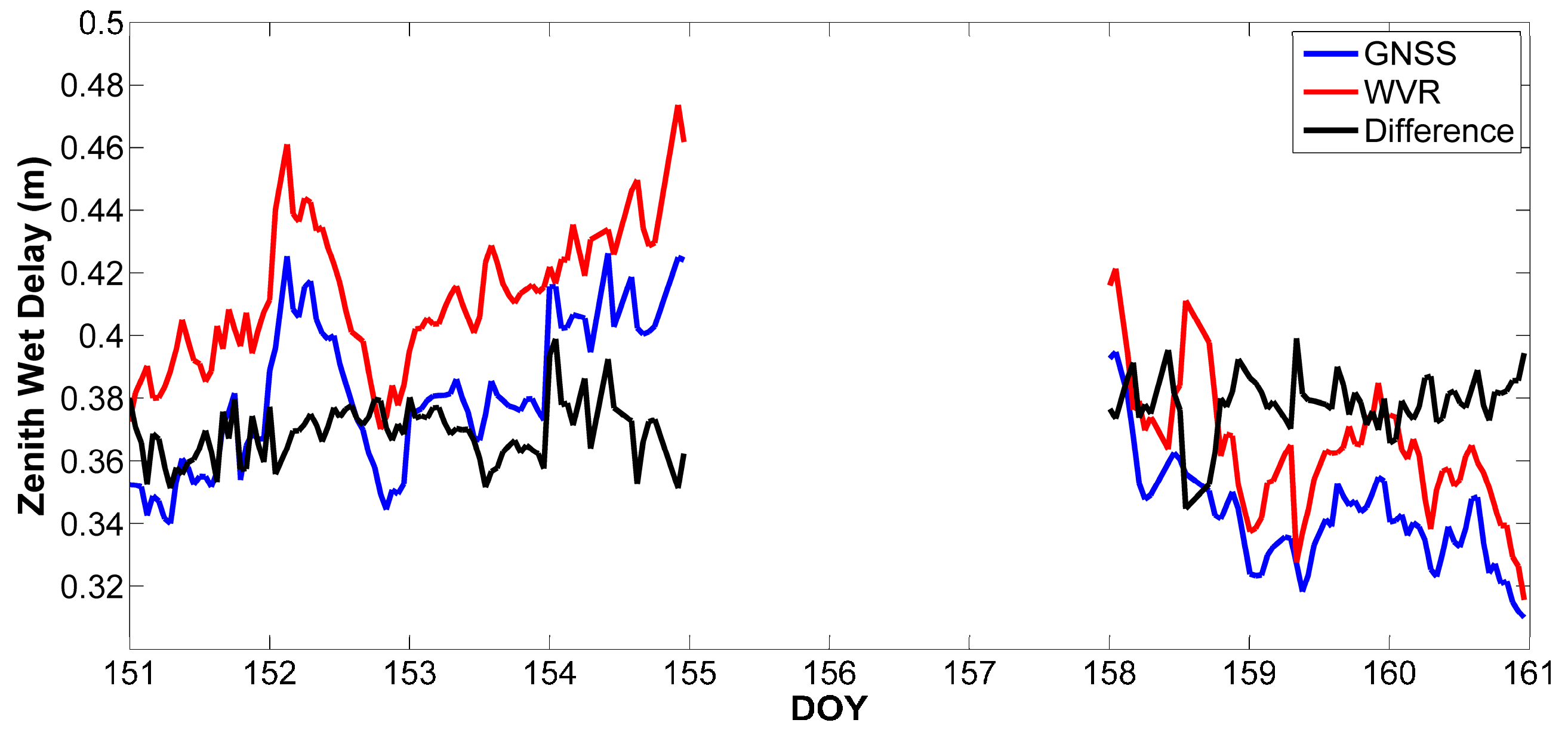
The GNSS- and water vapor radiometer (WVR)-derived wet troposphere delays were also compared (
Figure 7). The WVR instrument was developed by Radiometrics Corporation with five-band measurements that cover the frequency range of 22–30 GHz and was set up together with the Beigang GNSS permanent station. The distance between GNSS antenna and WVR instrument was about 3 m and the altitude was nearly the same. The wet troposphere delay was calculated from precipitable water vapor measured by WVR multiplied by a scale factor. The detail process refers to Yeh
et al. [
28]. The mean difference of GNSS and WVR observations is –2.70 cm with a STD of 1.04 cm and the correlation coefficient between them is 0.95. This comparison agrees with the finding of Chiang
et al. [
39] and Yeh
et al. [
28]. The discrepancy may be caused by that WVR measurements could be contaminated by surrounding buildings. Thus, the GNSS data processed by PPP can effectively estimate wet troposphere delay. Although the wet troposphere delay derived from GNSS data is underestimated compared with that derived by WVR observations as Yeh
et al. [
28] found, this issue does not affect the identification of LSA trends.
Figure 7.
Comparison of wet troposphere delays derived from GNSS and WVR in Yuanchang. The time span is from 30 May 2008 to June 8, 2008 (day of year (DOY): 151–160). Differences of GNSS- and WVR-derived wet troposphere delays (black curve) shift a constant value of 40 cm.
Figure 7.
Comparison of wet troposphere delays derived from GNSS and WVR in Yuanchang. The time span is from 30 May 2008 to June 8, 2008 (day of year (DOY): 151–160). Differences of GNSS- and WVR-derived wet troposphere delays (black curve) shift a constant value of 40 cm.
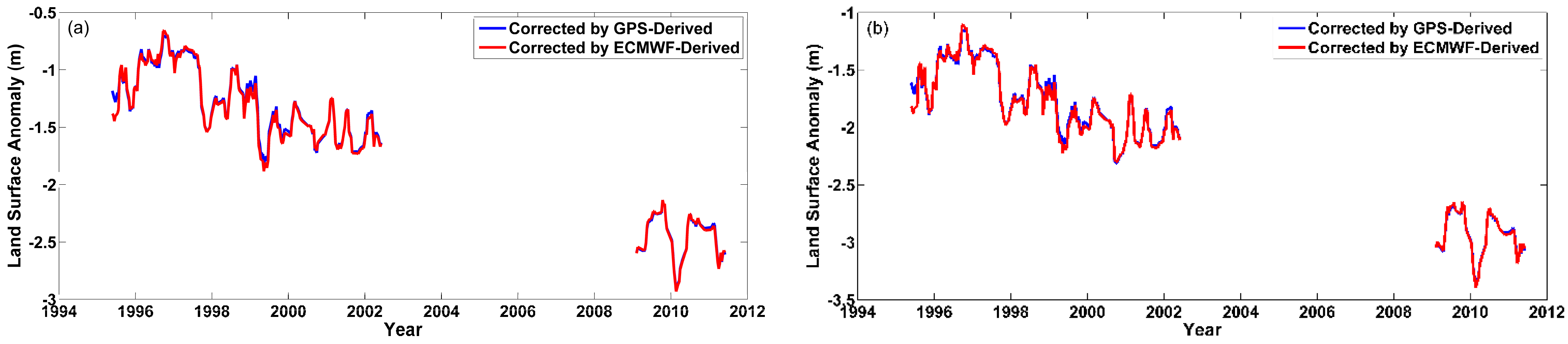
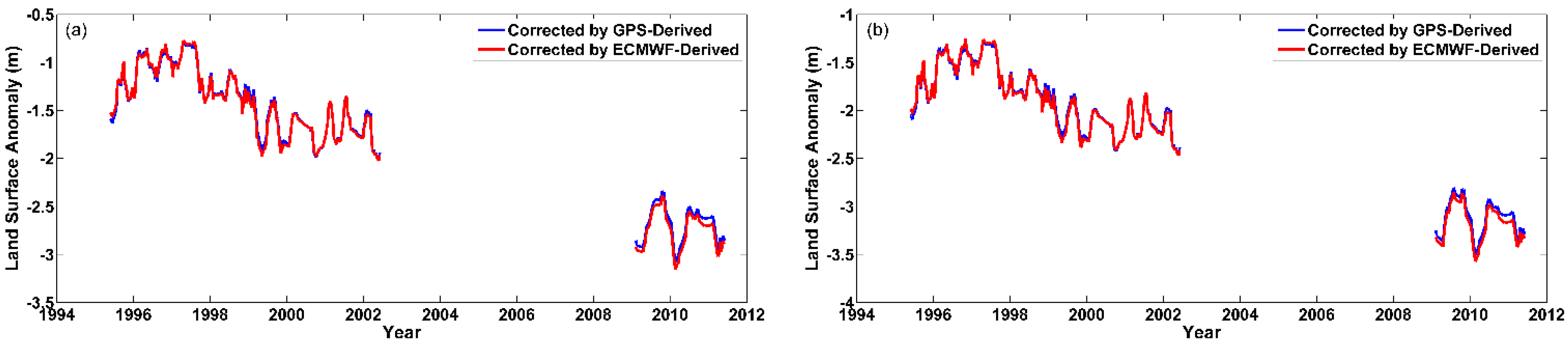
The wet troposphere delays derived from the GNSS data and ECMWF model were individually applied to the retracked altimetry data to evaluate the influence on land vertical motion trends. The time series of LSA in Yuanchang and Tuku are shown in
Figure 8 and
Figure 9, and the trends of LSA were calculated with six-parameter fitting, including the offset, annual, semi-annual, and trend (
Table 1).
Table 1 indicates that the rates and STDs of the vertical motion trends show no significant difference probably because the accuracy of retracked altimetric LSA is relatively worse than that of wet troposphere delay.
Figure 8.
Retracked altimetric LSAs corrected by GNSS- and ECMWF-derived wet troposphere delays in Yuanchang; (a) retracking by MTR; (b) retracking by STR. Blue and red curves represent the corrections of GNSS- and ECMWF-derived delays, respectively.
Figure 8.
Retracked altimetric LSAs corrected by GNSS- and ECMWF-derived wet troposphere delays in Yuanchang; (a) retracking by MTR; (b) retracking by STR. Blue and red curves represent the corrections of GNSS- and ECMWF-derived delays, respectively.
Figure 9.
Retracked altimetric LSA corrected by GNSS-derived and ECMWF wet troposphere delays in Tuku, (a) retracking by MTR; (b) retracking by STR. Blue and red curves represent the corrections of GNSS- and ECMWF-derived delays, respectively.
Figure 9.
Retracked altimetric LSA corrected by GNSS-derived and ECMWF wet troposphere delays in Tuku, (a) retracking by MTR; (b) retracking by STR. Blue and red curves represent the corrections of GNSS- and ECMWF-derived delays, respectively.
Table 1.
Trends of LSAs corrected by GNSS- and ECMWF-derived wet troposphere delays in Yuanchang and Tuku.
Table 1.
Trends of LSAs corrected by GNSS- and ECMWF-derived wet troposphere delays in Yuanchang and Tuku.
| | Trend (cm/yr) |
|---|
| Yuanchang | Tuku |
|---|
| MTR | STR | MTR | STR |
|---|
| ECMWF-derived | −10.09 ± 0.73 | −10.10 ± 0.70 | −11.62 ± 0.75 | −11.28 ± 0.71 |
| GNSS-Derived | −10.24 ± 0.69 | −10.28 ± 0.66 | −11.19 ± 0.75 | −10.85 ± 0.71 |
As seen in
Table 2, the STDs of land motion trends derived from satellite altimetry retracked by MTR and STR in the nine study regions are generally smaller than those of non-retracking LSA. The averaged STD of determined land motion trends reduces about 25% after waveform retracking. Therefore, the waveform retracking technique is helpful in improving accuracy of estimated vertical motion trends.
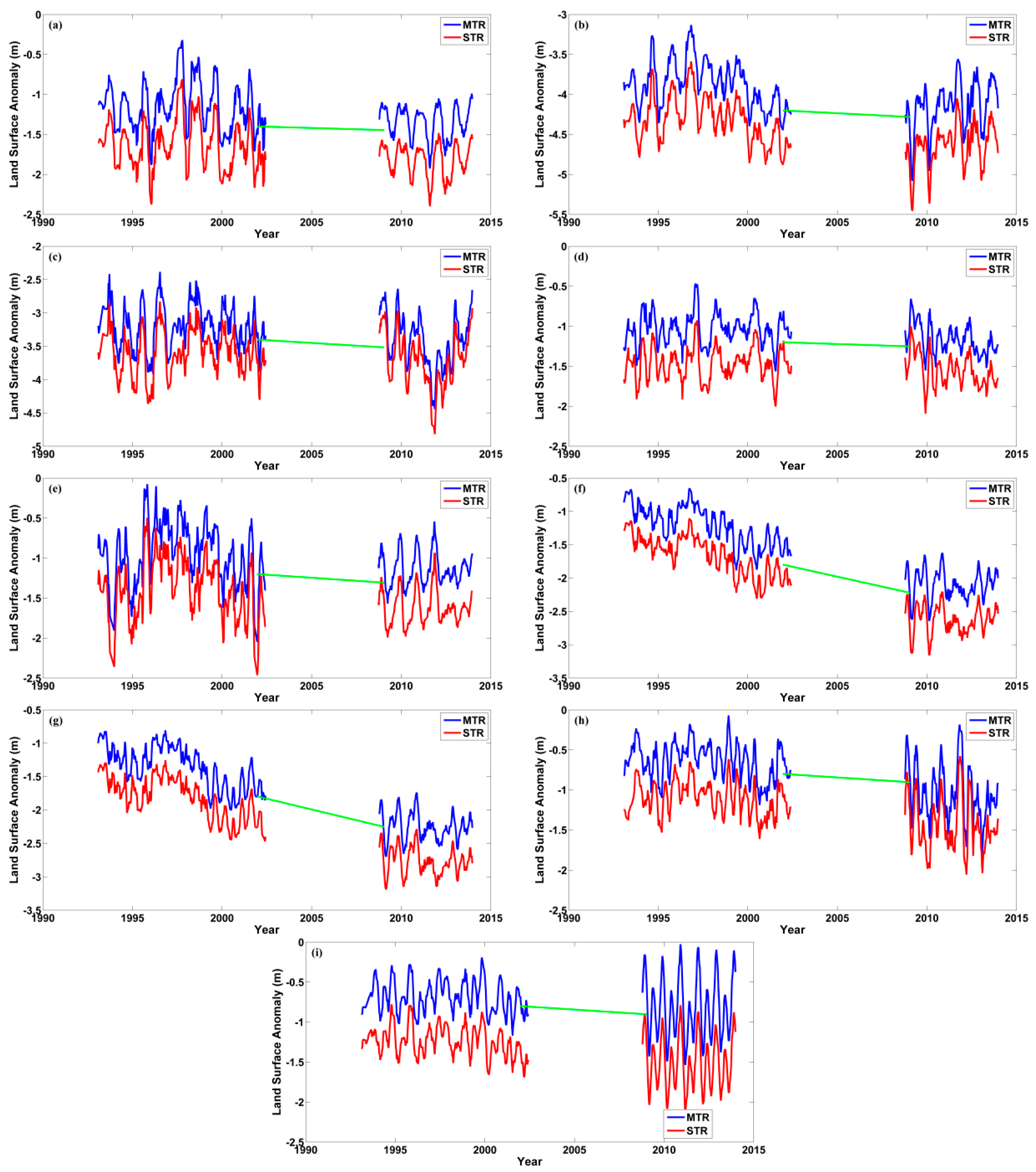
Figure 10 and
Table 2 also show that the LSAs retracked by MTR and STR agree well and the trend difference is not significant compared with the STD of the estimated trend. The trend difference could result from the calculation of thermal noise and the maximum power of the leading edge as well as the use of full waveform or subwaveform. In accordance with STDs of trends, STR performs slightly better than MTR. In the crossover region, STR outperforms MTR because the difference between trends of passes 51 and 164 is smaller at 0.51 cm/yr compared with 1.99 cm/yr. In addition to the errors of the satellite orbits, altimetry measurements, and corrections, the trend difference of passes 51 and 164 in the crossover region may be caused by the fact that the pass 164 ground track just now passes over the coastline from ocean to land before approaching the crossover area, which could degrade the altimetric accuracy. It should also be noted, since only a single comparison at one crossover is made, it cannot be confidently concluded which retracker is better. Aside from larger vertical motion rates and unrealistic annual signals, possibly due to the changes of covered vegetation, the variation of soil moisture, the nature of soil, and altimetry observation and correction errors, the possible reason for the larger STDs of the trends compared with the 2.9 mm/yr obtained by Lee
et al. [
11] is that the topography of the study area is rougher and the land cover is more complicated in the present study than in the study by Lee
et al. [
11]. Therefore, the study becomes challenging if the area is extremely rough (e.g., mountain region) or is covered by dense vegetation.
Figure 10.
Time series of the LSAs in the nine study regions derived from satellite altimetry retracked by MTR and STR. Green oblique lines represent the land motion derived from the leveling-derived trend rates as shown in
Figure 11. (
a) area 1; (
b) area 2; (
c) area 3; (
d) area 4; (
e) area 5; (
f) Yuanchang; (
g) Tuku; (
h) pass 51 in the crossover area; and (
i) pass 164 in the crossover area.
Table 2.
Trends of LSAs from retracked altimetry data in the nine study regions (unit: cm/yr).
Table 2.
Trends of LSAs from retracked altimetry data in the nine study regions (unit: cm/yr).
| | Study Region | Area 1 | Area 2 | Area 3 | Area 4 | Area 5 |
| Retracker | |
| MTR | −1.44 ± 0.58 | −2.07 ± 0.61 | −1.60 ± 0.74 | −0.94 ± 0.39 | −1.51 ± 0.66 |
| STR | −1.47 ± 0.57 | −2.47 ± 0.57 | −0.78 ± 0.74 | −0.59 ± 0.42 | −1.81 ± 0.65 |
| Non-retracking | −3.02 ± 0.73 | −1.17 ± 0.56 | 0.55 ± 0.76 | −1.49 ± 0.43 | 2.95 ± 1.10 |
| | Study Region | Yuanchang | Tuku | Cross 51 | Cross 164 | |
| Retracker | |
| MTR | −6.46 ± 0.44 | −6.61 ± 0.46 | −3.13 ± 0.54 | −1.14 ± 0.57 | |
| STR | −6.98 ± 0.41 | −6.96 ± 0.44 | −2.58 ± 0.52 | −2.07 ± 0.50 | |
| Non-retracking | −3.60 ± 0.80 | −3.86 ± 0.73 | −5.96 ± 0.77 | −2.50 ± 0.59 | |
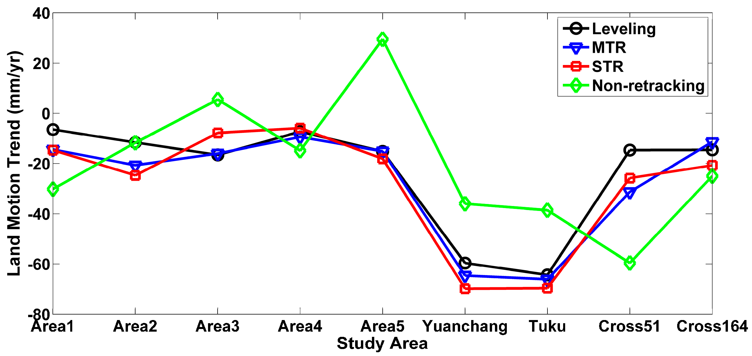
Figure 11.
Comparison of the vertical land motion trends in the nine study regions. The black, blue, red, and green curves represent the vertical motion trends derived from leveling, altimetry retracked by MTR and STR, and non-retracking altimetry, respectively.
Figure 11.
Comparison of the vertical land motion trends in the nine study regions. The black, blue, red, and green curves represent the vertical motion trends derived from leveling, altimetry retracked by MTR and STR, and non-retracking altimetry, respectively.
The vertical displacement rate field of Taiwan, regarded as independent measurements and calculated from the precise geodetic leveling data at 1843 solidly constructed benchmarks from 2000–2008 [
6], was used to evaluate the estimated vertical land motion trends from altimetry. Leveling-derived vertical motion rates at points of altimetry ground tracks in the nine study areas were estimated from the rates of 1843 benchmarks by cubic spline interpolation, and then the interpolated leveling-derived trends were averaged in each area, corresponding to the along-track space of 12 km or two 1-Hz LSAs, for comparison purposes (
Figure 11 and
Table 3). There is a large discrepancy between leveling-derived and non-retracking altimetric vertical motion trends, showing non-retracking altimetric data are not capable of monitoring land motions. After processed by the retrackers, the land motion trends from both measurements are consistent, with a correlation coefficient of 0.96. In addition, the mean trend differences between leveling-derived and altimetric vertical motion trends by MTR and STR are −0.43 and −0.52 cm/yr, with STDs of 0.61 and 0.69 cm/yr, respectively. The STD reduces about 75% compared with the one from non-retracking altimetric measurements and both retrackers perform equally well. If reflected waveforms are complex and contain multiple peaks, STR will perform better in theory; however, if extracted subwaveform wrongly represents the leading edge, the calculated range correction could be biased. In the study, since multi-peak waveforms were seen as outliers when MTR was used, the results derived from both retrackers show no significant difference. The mean difference between leveling and retracked altimetric measurements ranges from −4 mm/yr to −5 mm/yr, which is consistent with that found by Ching
et al. [
4]. A bias of approximately −4 mm/yr between the GNSS- and leveling-derived vertical motion rates can be ascribed to the relative vertical motion rates derived from leveling data referring to the original benchmark. In order to evaluate the error budget resulting from observations covering different time spans, we first fitted the time series of altimetric LSAs retracked by MTR and STR to a model of six parameters plus an acceleration term (seven parameters in total). The LSA time series covering 2002–2008 in nine study areas, which were reconstructed using the seven estimated parameters, were then used to estimate the linear trends by six-parameter fitting. Comparing the leveling-derived trends with the reconstructed LSA-derived trends, the mean trend differences are −0.46 and −0.52 cm/yr, with STDs of 0.64 and 0.64 cm/yr, respectively, showing no significant difference compared with the values in
Table 3. It indicates that the trend difference resulting from the use of observations covering different time spans in our study is relatively small and negligible.
Table 3.
Mean differences and correlation coefficients between the vertical motion trends derived from leveling and retracked altimetry in the nine study areas.
Table 3.
Mean differences and correlation coefficients between the vertical motion trends derived from leveling and retracked altimetry in the nine study areas.
| | Mean of Differences with STD (cm/yr) | Correlation Coefficient |
|---|
| MTR-LSA | −0.43 ± 0.61 | 0.96 |
| STR-LSA | −0.52 ± 0.69 | 0.96 |
| Non-retracking-LSA | 0.33 ± 2.82 | 0.33 |


