4.1. Direct Validation of LAI3g as Compared to LAI GGRS
The validation of LAI3g and LAI GGRS with ground-based LAI datasets was carried out by performing regression analysis between LAI from both products (dependent variables) and LAI derived from Landsat (independent variables). The detailed results obtained from this validation are summarized in
Table 4 and
Figure 2 and
Figure 3.
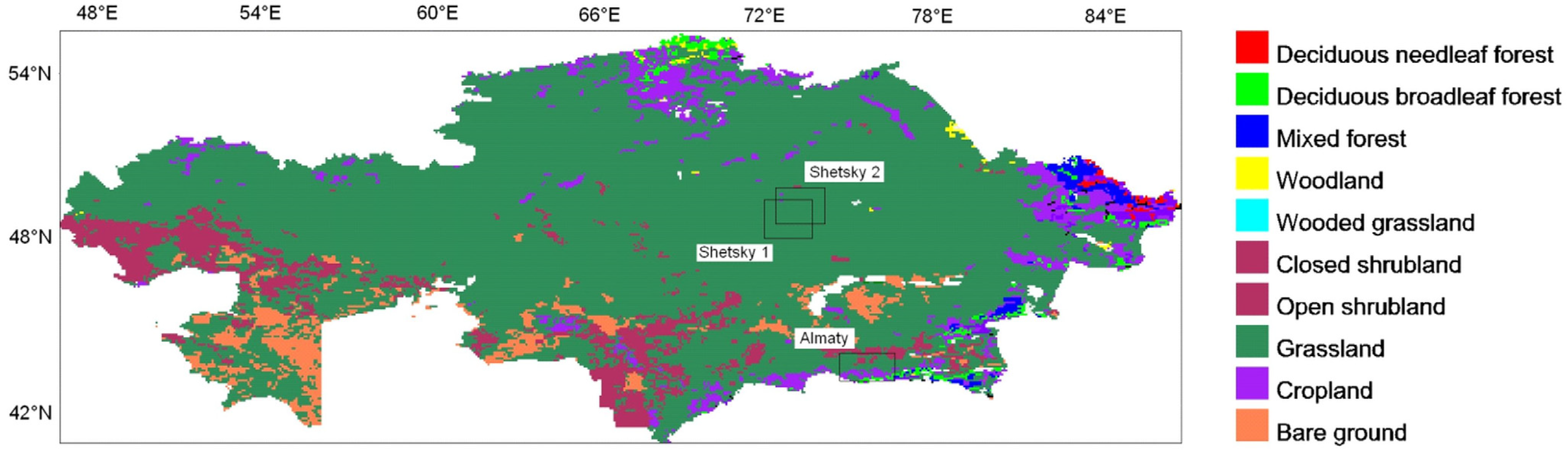
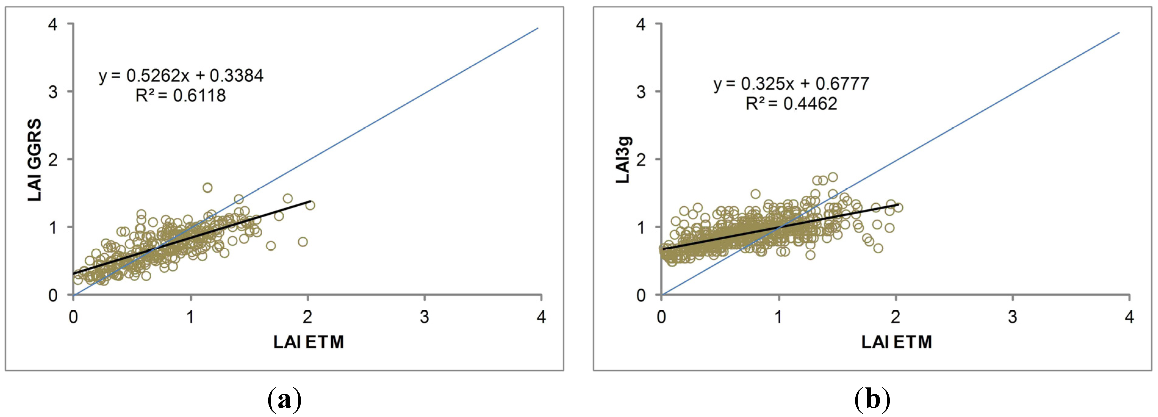
Figure 2 shows scatter plots for the pixel-by-pixel comparisons of the LAI products with the spatially-degraded Landsat-derived LAI map from the Shetsky validation site in Central Kazakhstan dominated by grassland, while
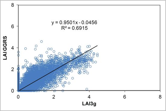
Figure 3 presents the scatter plots from the Almaty validation site in southern Kazakhstan, with forest cover being dominant.
The results indicate a generally significant correspondence between both LAI products and the Landsat-derived LAI maps in both validation sites. However, the analyses detect that the LAI3g product has much weaker relations with the Landsat LAI in both validation sites, indicating poorer replication of the ground-based LAI by LAI3g dataset, as compared to the LAI GGRS product. Comparisons of LAI3g with the Landsat-derived LAI are characterized by lower values of
R2 and higher values of RMSE in both validation sites. The difference between the LAI3g and LAI GGRS validation results is much more pronounced for the Almaty validation site. Thus, LAI3g reproduces only 25% of the variance contained in the Landsat-derived LAI, whereas LAI GGRS reproduces 69% of the variance. The RMSE value of LAI3g is much higher than for LAI GGRS (1.55 and 0.70). In terms of relative RMSE (RMSE% = 98%), the validation results of LAI3g in the Almaty test site detect that the user consistency requirements are not fulfilled (RMSE > 0.5 LAI). For other comparisons, differences between the LAI products and the Landsat-derived LAI maps are lower than 0.5 LAI in terms of RMSE, fulfilling user consistency requirements for LAI estimates [
23].
Figure 2.
Validation of LAI products over grassland in the Shetsky test region for June 2008. Pixel-by-pixel (n = 720) comparison of the aggregated fine-resolution Landsat-derived LAI map versus the LAI GGRS product (a); and versus the LAI3g product (b).
Figure 2.
Validation of LAI products over grassland in the Shetsky test region for June 2008. Pixel-by-pixel (n = 720) comparison of the aggregated fine-resolution Landsat-derived LAI map versus the LAI GGRS product (a); and versus the LAI3g product (b).
Figure 3.
Validation of LAI products over forests in the Almaty test region for August 2010. Pixel-by-pixel (n = 846) comparison of the aggregated fine-resolution Landsat-derived LAI map versus the LAI GGRS product (a); and versus the LAI3g product (b).
Figure 3.
Validation of LAI products over forests in the Almaty test region for August 2010. Pixel-by-pixel (n = 846) comparison of the aggregated fine-resolution Landsat-derived LAI map versus the LAI GGRS product (a); and versus the LAI3g product (b).
The analyses detect statistically-significant positive values of offset for both LAI3g and LAI GGRS comparisons in both validation sites, indicating a higher estimation of low LAI values in the coarse-resolution LAI products as compared to the Landsat-derived LAI for both sites. The magnitude of difference is quite high for LAI3g in both validation sites (offset value of 0.67 versus 0.33 and 0.91 versus 0.41 for LAI3g and LAI GGRS, respectively). In all analyses, slope values are <1.0, indicating a significantly lower estimation of the high values of Landsat-derived LAI by both LAI3g and LAI GGRS retrievals. As compared to LAI3g, the magnitude of the difference is much lower by LAI GGRS for both validation sites (slope values of 0.33 versus 0.53 and 0.38 versus 0.63 for LAI3g and LAI GGRS, at Sites 1 and 2 respectively).
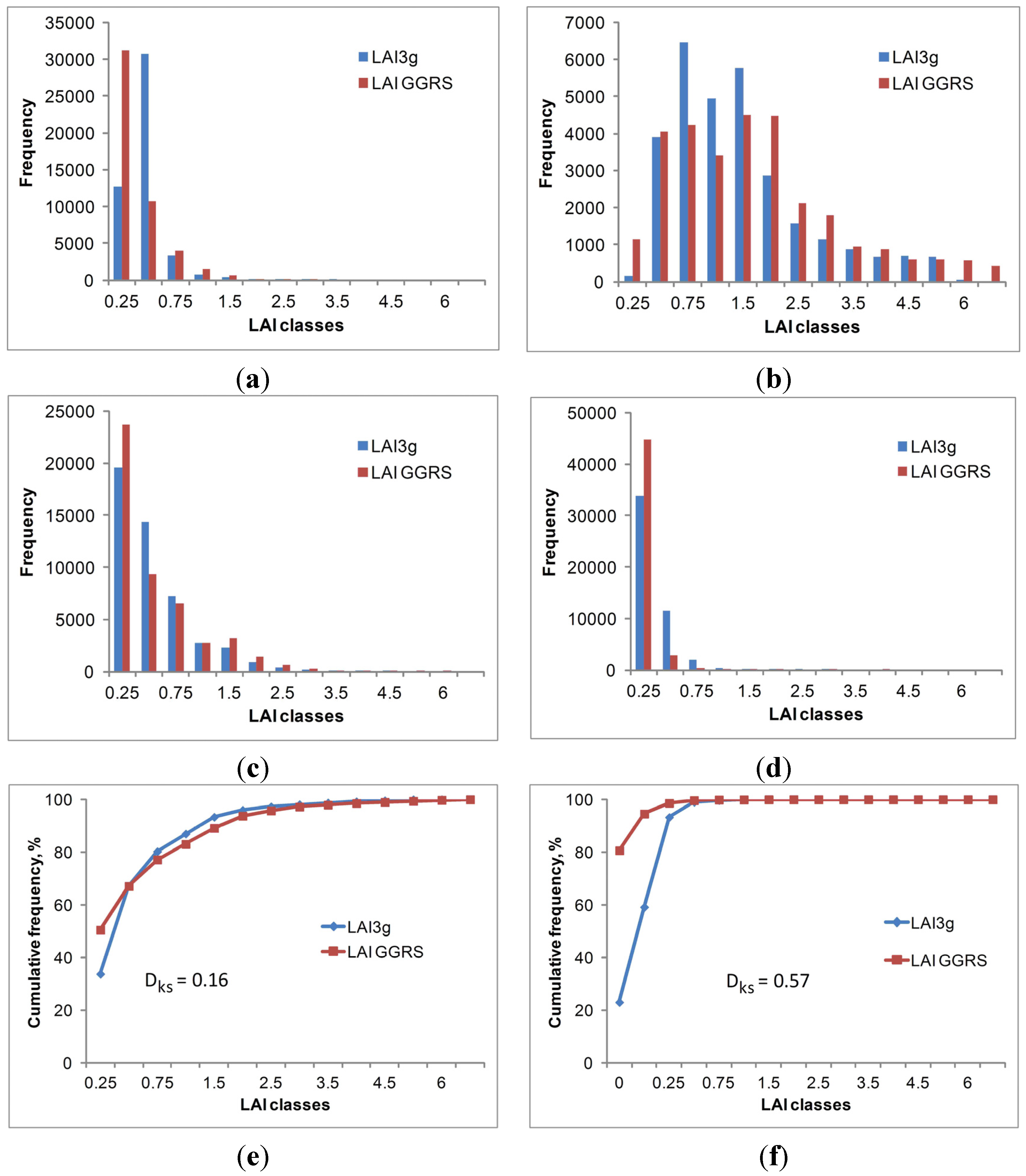
The better predictions of LAI by LAI GGRS than by LAI3g retrievals are also reflected in the comparisons of LAI histograms from the validation sites (
Figure 4). The histograms reveal that the LAI distribution of the LAI GGRS datasets is generally consistent with that of the Landsat-derived LAI datasets in both validation sites, whereas LAI3g distributions are characterized by significant discrepancies with the independent datasets. In the Shetsky test site, the LAI3g histogram shows a sharp-peaked form with a much higher frequency in the value classes 0.5 < LAI < 0.75, 0.75 < LAI < 1.0 and 1.0 < LAI < 1.25 in comparison to the Landsat-derived LAI histograms, while the LAI classes at the left and right side ranges are occupied only slightly. This is also reflected in statistics of the datasets in the Shetsky test area. LAI3g has a mean value of 0.91 with a standard deviation of 0.2
versus a mean value of 0.76 and a standard deviation of 0.31 for LAI GGRS. The statistics of LAI GGRS are much closer to those of LAI ETM+ (mean value of 0.66, standard deviation of 0.43) than the statistics of LAI3g. In the Almaty test site, the LAI3g histogram is characterized by very low frequency of pixels in the lowest LAI class (0 < LAI < 0.25) and excessively high frequency in the third and fourth LAI classes (0.5 < LAI < 0.75 and 0.75 < LAI < 1.0), which is contrary to the Landsat based histogram. The LAI GGRS histogram demonstrates much more similarity with the LAI ETM+ histogram in all value classes (
Figure 4b). The LAI value range of LAI3g estimates (0 ≤ LAI ≤ 4.7) is significantly lower than that of the ETM+ LAI reference dataset (0 ≤ LAI ≤ 6.5), highlighting the relatively poor capability of LAI3g to replicate the LAI ETM+ values.
The data distribution is also examined comparing the ECDFs from both validation sites (
Figure 4c,d). Generally, for both test sites, the ECDF of LAI GGRS shows much better correspondence with the ECDF of the Landsat-derived LAI than LAI3g. This is reflected in values of the Kolmogorov–Smirnov statistic (D
KS), which are considerably lower for the LAI GGRS product. LAI3g demonstrates larger differences in ECDF shapes to Landsat-derived LAI; they are particularly noticeable at the Shetsky test site (
Figure 4c). However, the two-sample Kolmogorov–Smirnov test at the 5% significance level accepted the null hypothesis that ECDFs have the same continuous distribution, revealing a general agreement of both LAI products with the Landsat-derived LAI.
In order to support the analyses of the regressions and histograms, we also conducted
F-tests of variance equality. Results of the
F-tests are shown in
Table 5. The results revealed a statistically-significant correspondence between the compared datasets: for all cases, the obtained
F-value was lower than the critical
F-value, detecting that the null hypothesis (H
o = datasets have similar variance) should be accepted.
In order to support the analyses of the regressions and histograms, we also conducted
F-tests of variance equality. Results of the
F-tests are shown in
Table 5 and are valid at the 95% confidence level. The results revealed a statistically-significant correspondence between the compared datasets, except LAI3g for the Almaty test site. Here, the obtained
F-value was higher than the critical
F-value, detecting that the null hypothesis (H
o = datasets have similar variance) should be rejected.
Figure 4.
Frequency distributions (a,b) and empirical cumulative distribution functions (c,d) of Landsat-based LAI, LAI GGRS and LAI3g products at the Shetsky and Almaty validation sites.
Figure 4.
Frequency distributions (a,b) and empirical cumulative distribution functions (c,d) of Landsat-based LAI, LAI GGRS and LAI3g products at the Shetsky and Almaty validation sites.
Table 4.
Validation results of LAI3g and LAI GGRS datasets versus the ground-based LAI up-scaled using Landsat imagery.
Table 4.
Validation results of LAI3g and LAI GGRS datasets versus the ground-based LAI up-scaled using Landsat imagery.
| Validation Site/Dominate Land Cover | Month/Year | LAI Product | Offset | Slope | R2 | RMSE/RMSE% |
|---|
| Shetsky/Grassland | June/2008 | LAI3g | 0.67 | 0.33 | 0.44 | 0.37/49% |
| LAI GGRS | 0.33 | 0.53 | 0.61 | 0.24/31% |
| Almaty/Forest | August/2010 | LAI3g | 0.91 | 0.38 | 0.25 | 1.55/98% |
| LAI GGRS | 0.41 | 0.63 | 0.69 | 0.71/43% |
Table 5.
Test statistics and results of the F-test conducted for a comparison of the LAI3g and the LAI GGRS product versus the ground-based up-scaled Landsat LAI. The null hypothesis of variance equality is accepted when F-value < critical F-value.
Table 5.
Test statistics and results of the F-test conducted for a comparison of the LAI3g and the LAI GGRS product versus the ground-based up-scaled Landsat LAI. The null hypothesis of variance equality is accepted when F-value < critical F-value.
| Validation Site | LAI product | Mean LAI | Variance | F-value | Critical F-value |
|---|
| Shetsky | Landsat LAI | 0.74 | 0.17 | | |
| LAI3g | 0.92 | 0.07 | 0.23 | 0.88 |
| LAI GGRS | 0.75 | 0.12 | 0.18 | 0.88 |
| Almaty | Landsat LAI | 1.71 | 1.66 | | |
| LAI3g | 1.52 | 1.01 | 0.90 | 0.88 |
| LAI GGRS | 1.51 | 1.17 | 0.68 | 0.88 |
4.2. Comparison of LAI3g and LAI GGRS
The following comparison between the LAI3g and the LAI-GGRS is grouped in terms of spatial and temporal components. For spatial comparison, we used the following three procedures. First, the spatial frequency is compared followed by the spatial analysis based on per pixel comparison being computed. Second, pixel-by-pixel comparisons of both LAI products for the year 2008 were carried out using regression analysis and corresponding scatter plots. Root mean square error (RMSE), the coefficient of determination (R2), the slope of the regression line and intercept were used as guides of statistical association between the LAI products. To assess spatial agreement between the products, AC was calculated for each of the months. The analysis of the temporal evolution of AC aimed to highlight specific periods of spatial disagreement. In addition to these analyses, F-tests were conducted for each month from 2008 to test the equality of variances between monthly LAI products. The F-tests included all pixels within the territory of Kazakhstan. The null hypothesis that implies the statistically-significant equality of the datasets was rejected when an F-value was higher than a critical F-value.
In addition to these analyses, F-tests were conducted for each month from 2008 to test the equality of variances between monthly LAI products. The F-tests included all pixels within the territory of Kazakhstan. The null hypothesis that implies the statistically-significant equality of the datasets was rejected when an F-value was higher than a critical F-value. Third, differences between LAI3g and LAI GGRS datasets for the individual months over the year 2008 were produced, and LAI difference maps were analyzed. For temporal comparison, we produced seasonal trajectories of LAI3g and LAI GGRS for different land cover types during the period 2005–2008.
4.2.1. Spatial Frequency
In general, the analyzed LAI histograms revealed similar trends between the LAI datasets. Nonetheless, there also are some important differences between the datasets, which are reflected in
Figure 5, which shows the LAI histograms for LAI3g and LAI GGRS products in four specific months that cover the main vegetation growing period (April to October) over the area of Kazakhstan. Frequency is given as the total number of pixels over the area of Kazakhstan.
For both LAI products, the frequency of the lowest LAI values is very high at the start and the end of the growing season (
Figure 5a,d). It decreases during summer months (
Figure 5c) and has the minimum at the peak of the growing season (
Figure 5b). These results are consistent with other LAI products [
24,
25] and reflect the seasonality of vegetation growth in temperate climate zones. The largest histogram differences between the two LAI products occur at the beginning of the growing season during April (
Figure 5a), when LAI3g shows a much lower frequency of LAI retrievals within the lowest LAI class (0 < LAI < 0.25) than does LAI GGRS. The second lowest LAI class (0.25 < LAI < 0.5) of the LAI3g histogram is characterized by a much higher frequency as compared to LAI GGRS. Most of the LAI3g pixels belong to this LAI class, whereas LAI GGRS has greatest number of its pixels within the lowest LAI class. The LAI3g product continually, and significantly, exceeds LAI GGRS, also at the end of the growing season in October (
Figure 5d). LAI3g shows a much lower frequency of retrievals with LAI < 0.25 and a much higher frequency of retrievals with LAI > 0.25 than does LAI GGRS. This means that the LAI3g product tends to produce generally higher LAI values at the beginning and at the end of the growing season than does LAI GGRS.
Figure 5.
Comparison of the LAI3g/GGRS-LAI value distribution over Kazakhstan: distribution histograms for (a) April, (b) June, (c) August, (d) October (e) and (f) empirical cumulative distribution functions (ECDFs). Number of samples: 48,000. In (e), the months from the growing season (April–October) and in (f) the months from the leafless phase (November–March) are pooled together. Number of samples: 48,000.
The June histograms represent the maximum LAI values over the Kazakhstan territory (
Figure 5b); therefore, among all months, they are characterized by the broadest range of values. Both LAI3g and LAI GGRS June histograms show a log-normal distribution. However, there are some differences between the June histograms: the LAI3g histogram shows a sharper kurtosis, while the LAI GGRS histogram shows a continuous and smooth frequency distribution. Most LAI3g pixels are concentrated in the lowest four LAI classes (from 0.25 to 1.5), whereas the other LAI classes (from 2.0 to >6.0) are occupied more rarely. As compared to LAI3g, the LAI GGRS shows lower frequency in the lower LAI classes and higher frequency in all other classes (
Figure 5b). The greatest differences existing between the two LAI histograms is observed in the peak LAI class (0.25 < LAI < 0.5): here, the pixel frequency of the LAI GGRS product is almost two-times lower than that of the LAI3g product. The differences between the June histograms are also reflected in the calculated statistics: the histogram kurtosis of LAI3g has a value of 8.7
versus 5.2 for the LAI GGRS histogram; the histogram shift of LAI3g is 2.5
versus 2.0 for the LAI GGRS histogram. These results show that, in contradiction to a sharp-peaked histogram of LAI3g, LAI GGRS is characterized by a flattened distribution of pixels within the LAI classes. Other statistics also confirmed some significant differences between the June LAI datasets. Thus, the June LAI3g is characterized by a mean value of 0.78 (
p < 0.01) and a standard deviation of 0.69, while the June LAI GGRS has a mean of 1.03 (
p < 0.01) and a standard deviation of 0.94. The August histograms also reveal some differences between both LAI products (
Figure 5c); however, these differences are not as significant as for the April and October histograms. All in all, the histogram analyses detected a higher similarity between both LAI products during the summer months and a lower similarity between LAI3g and LAI GGRS at the beginning and at the end of the growing season. The overall data distribution is examined comparing the ECDFs, where the months from the growing season and from the leafless phase (November–March) are pulled together (
Figure 5e,f). For the growing season months, LAI3g values are lower than the corresponding LAI GGRS for the first left-side class (0 < LAI < 0.25) and somewhat higher for the middle-range classes (0.75 < LAI < 3.5). For the leafless period, differences between LAI3g and LAI GGRS are enormous. The LAI GGRS ECDF contains the greatest number of the pixels (over 80%) in the first class (LAI = 0) and 14% of all pixels in the second class (0 < LAI < 0.1), whereas the LAI3g ECDF shows that the greatest number of pixels is contained in the second and third classes (0 < LAI < 0.1, 0.1 < LAI < 0.25, respectively), and the first class contains only 23%. This means that the LAI3g product detects green vegetation in the most part of the territory of Kazakhstan, whereas the LAI GGRS product does not. Quantitatively, differences in ECDFs are described by the Kolmogorov–Smirnov statistic (D
KS) presented in
Figure 5. For the growing season ECDFs, the two-sample Kolmogorov–Smirnov test at the 5% significance level accepted the null hypothesis that ECDFs are from the same continuous distribution. For the leafless period, the null hypothesis was rejected, detecting statistically-significant differences between the LAI3g and LAI GGRS distributions.
4.2.2. Spatial Agreement between the LAI3g and GGRS-LAI
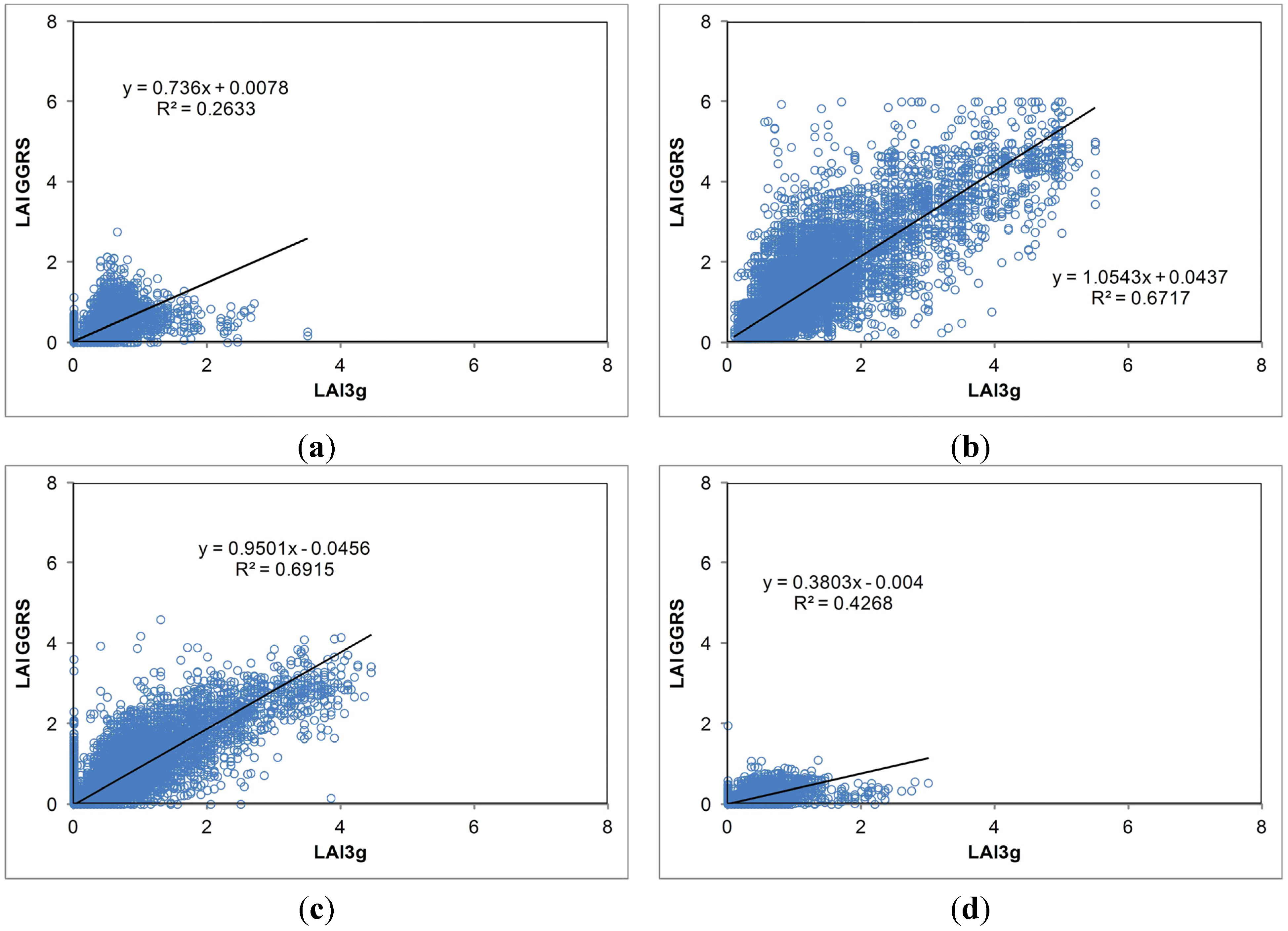
Pixel-by-pixel comparisons of both LAI products for the year 2008 supported the results of histogram analyses (
Section 4.2.1). Spatial agreement between both LAI products is much lower in April (
Figure 6a) and October (
Figure 6d) than during the summer months (
Figure 6b,c). As compared to the LAI GGRS retrievals, LAI3g tends to a higher frequency of estimates of low LAI values in April and October. The estimation of higher LAI values is particularly pronounced in October, where the regression line slope (0.38) is very different from the 1:1 line. As for April, the regression line slope (0.74) is somewhat closer to the 1:1 line. However, the April scatter plot displays more considerable scattering of data points around the regression line, detecting worse correspondence between both LAI products in this month (
R2 = 0.26 for April
versus R2 = 0.42 for October).
Contrary to the April and October comparisons, the June and August scatter plots (
Figure 6b,c) demonstrate a better agreement between LAI retrievals of the products. The regression line slope is very close to a value of 1.0 for both June and August (1.05 and 0.93, respectively), indicating good correspondence between both LAI products in the whole range of LAI retrievals. Nonetheless, some differences were detected between the products as detected in the histogram analyses (
Section 4.2.1). These differences are highlighted by the scattering of data points.
Figure 6.
Comparison of LAI3g and LAI GGRS over the whole area of Kazakhstan for specific months in 2008: (a) April; (b) June; (c) August; and (d) October. Number of samples: 48,000.
Figure 6.
Comparison of LAI3g and LAI GGRS over the whole area of Kazakhstan for specific months in 2008: (a) April; (b) June; (c) August; and (d) October. Number of samples: 48,000.
Both June and August comparisons revealed much better correspondence between the LAI datasets with RMSE values of 0.42 (43%) and 0.35 (48%) than the April and October retrievals. For these months, differences between LAI3g and LAI GGRS are lower than 0.5 LAI in terms of RMSE, fulfilling user consistency requirements for LAI estimates from multiple sensors [
22]. RMSE values of the April (0.22% or 66% in terms of relative RMSE) and October (0.21% or 92%) analyses are higher than 0.5LAI, detecting that the user consistency requirements are not fulfilled in these months.
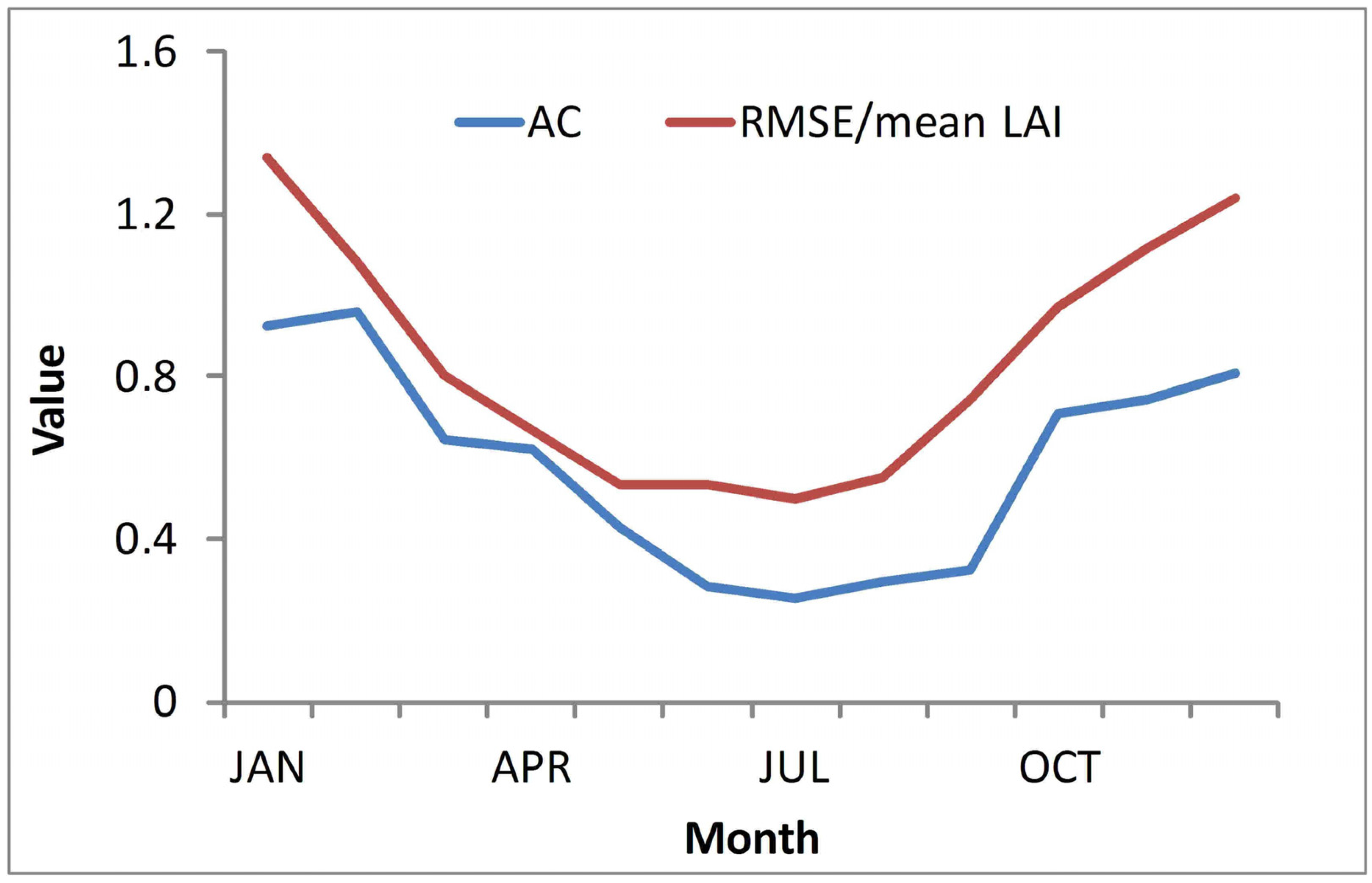
Figure 7 reports the temporal profiles of the agreement coefficient (AC) and the RMSE. Both statistics demonstrate similar dynamics with a pronounced seasonality. Periods of minimum agreement between LAI3g and LAI GGRS are found during wintertime, while spring/autumn months outside the growing season are characterized by a low agreement. In fact, during these periods, the two datasets provide quite different LAI dynamics. In particular, during wintertime LAI GGRS minima, LAI3g presents increasing LAI values. This overestimation by the LAI3g product can also be seen in the temporal profiles of LAI from different land cover classes (see section 4.2.4). A possible explanation for this effect may be that, during wintertime and months with a temperature <0°C, LAI GGRS applies a threshold of LAI = 0 for all non-woody land covers, suggesting no existence of green vegetation during the leafless phase. Obviously, LAI3g does not apply any filter or threshold that could adequately deal with imaginary vegetation during the leafless phase.
Figure 7.
Temporal profiles of the agreement coefficient (AC) and RMSE/mean LAI between LAI3g and LAI GGRS for 2008 over Kazakhstan.
Figure 7.
Temporal profiles of the agreement coefficient (AC) and RMSE/mean LAI between LAI3g and LAI GGRS for 2008 over Kazakhstan.
The above results are supported by the results of the
F-tests (
Table 6). The growing season months (April–September, except October) are characterized by statistically-significant similarity of LAI variance in both products. In contradiction to these, the LAI products of the months outside the growing season (October–March) reveal statistically-significant differences. Further analyses below (see
Section 4.2.3 and
Figure 7) provide additional evidence for the similarity/difference of the LAI products.
4.2.3. Spatial Differences between the LAI Products
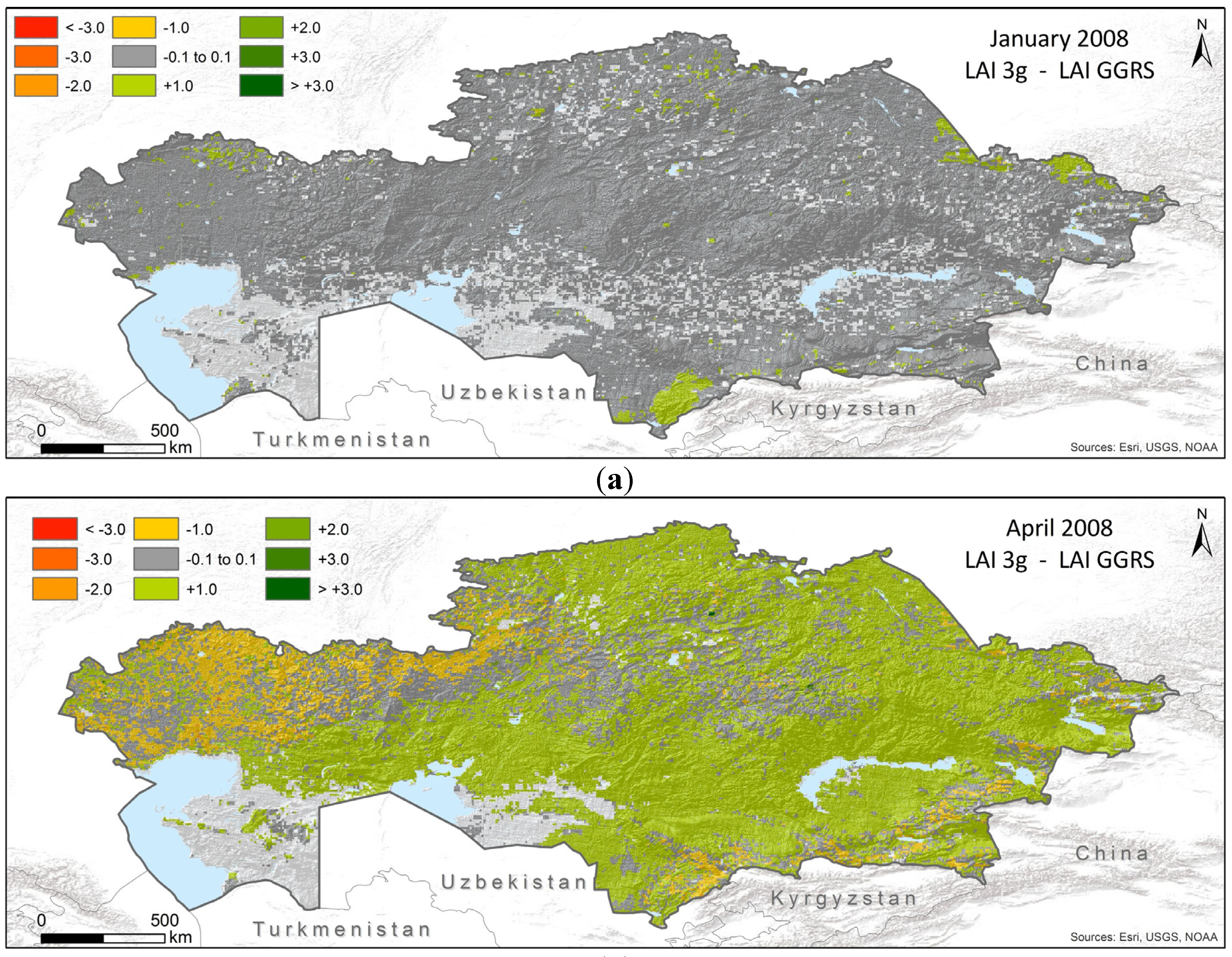
Spatial differences between LAI3g and LAI GGRS products at the pixel scale for specific months in 2008 are shown in
Figure 8. Thus, in
Figure 8a, we see a very regular distribution of green-colored pixels (0.056–0.13) over the whole territory of Kazakhstan with the exception of some pixels presented as the yellow class (0.14–0.23) in the forested areas in the southern and eastern parts of the country. A similar picture is apparent for the other winter months. In general, this is because LAI3g tends to show values of LAI > 0 for grassland and semi-desert biomes in winter months, while LAI GGRS does not (compare also with
Figure 9).
Table 6.
Test statistics and results of the F-test carried out for a comparison of the LAI3g versus the LAI GGRS product. The number of samples used for the comparison is 48,000. The null hypothesis is accepted for marked months (F-value < critical F-value).
Table 6.
Test statistics and results of the F-test carried out for a comparison of the LAI3g versus the LAI GGRS product. The number of samples used for the comparison is 48,000. The null hypothesis is accepted for marked months (F-value < critical F-value).
| Month | LAI Product | Mean LAI | Variance | F-value | Critical F-value |
|---|
| January | LAI3g/LAI GGRS | 0.085/0.005 | 0.0049/0.0005 | 9.35 | 1.01 |
| February | LAI3g/LAI GGRS | 0.088/0.0038 | 0.0061/0.0005 | 12.45 | 1.01 |
| March | LAI3g/LAI GGRS | 0.327/0.034 | 0.0694/0.0077 | 8.99 | 1.01 |
| April | LAI3g/LAI GGRS | 0.343/0.225 | 0.0387/0.0610 | 0.63 | 0.98 |
| May | LAI3g/LAI GGRS | 0.644/0.695 | 0.344/0.659 | 0.522 | 0.98 |
| June | LAI3g/LAI GGRS | 0.788/1.032 | 0.476/0.884 | 0.539 | 0.98 |
| July | LAI3g/LAI GGRS | 1.076/1.069 | 1.632/1.856 | 0.879 | 0.98 |
| August | LAI3g/LAI GGRS | 0.435/0.377 | 0.225/0.297 | 0.762 | 0.98 |
| September | LAI3g/LAI GGRS | 0.421/0.321 | 0.213/0.187 | 1.00 | 1.01 |
| October | LAI3g/LAI GGRS | 0.217/0.074 | 0.031/0.011 | 3.00 | 1.01 |
| November | LAI3g/LAI GGRS | 0.181/0.049 | 0.022/0.011 | 2.177 | 1.01 |
| December | LAI3g/LAI GGRS | 0.136/0.014 | 0.0086/0.0021 | 4.11 | 1.01 |
Figure 8.
Differences (LAI3g minus LAI GGRS) between the compared LAI products for specific months in 2008: (a) January; (b) April; (c) June; (d) August; and (e) October.
Figure 8.
Differences (LAI3g minus LAI GGRS) between the compared LAI products for specific months in 2008: (a) January; (b) April; (c) June; (d) August; and (e) October.
LAI3g is characterized by sensitivity to an earlier and more rapid start of the growing season in grassland/shrubland than LAI GGRS. This is reflected in the considerably greater values of LAI3g for these biomes in spring months (see, as an example, April in
Figure 8b), whereas LAI of both products for forest areas is characterized by only very small differences. In April, LAI3g of grasslands estimated values of LAI >> 0.5, while LAI GGRS shows significantly lower values (0.2 < LAI < 0.5) (compare also
Figure 9). This leads to a considerable broad-scale overestimation of LAI GGRS by the LAI3g product. LAI values of forest areas in the southern (mountainous) and northern parts of Kazakhstan seem to have only little differences between both LAI products.
The summer months (June and August in
Figure 8c,d) are characterized by diverse spatial patterns in the differences between LAI3g and LAI GGRS. Thus, large areas of mixed grasslands in northern Kazakhstan demonstrate in June somewhat lower values of LAI3g than LAI GGRS (yellow color), whereas other areas of grassland are characterized by a small difference between LAI GGRS and LAI3g (reddish color). Nonetheless, some areas of LAI3g show considerably higher values of LAI than LAI GGRS (red color). These areas are mostly located in cropland in the southern and middle parts of Kazakhstan.
Autumn, similarly to the spring, is characterized by significantly higher values of LAI3g in comparison to LAI GGRS (
Figure 8e). Higher values of LAI estimates presented by LAI3g range from 0.03 to 0.16 (green color) in the short grassland (central part of Kazakhstan) to 0.17–0.36 (yellow color) in the mixed and long grassland in the northern Kazakhstan. The reason for the generally higher values of LAI3g for autumn is the considerably slower decrease of LAI in the last phase of the growing season. The LAI difference image in
Figure 8c supports the scatter plot in
Figure 6d, demonstrating the overall overestimation of LAI GGRS by LAI3g.
4.2.4. Temporal Agreement: Seasonal Trajectories
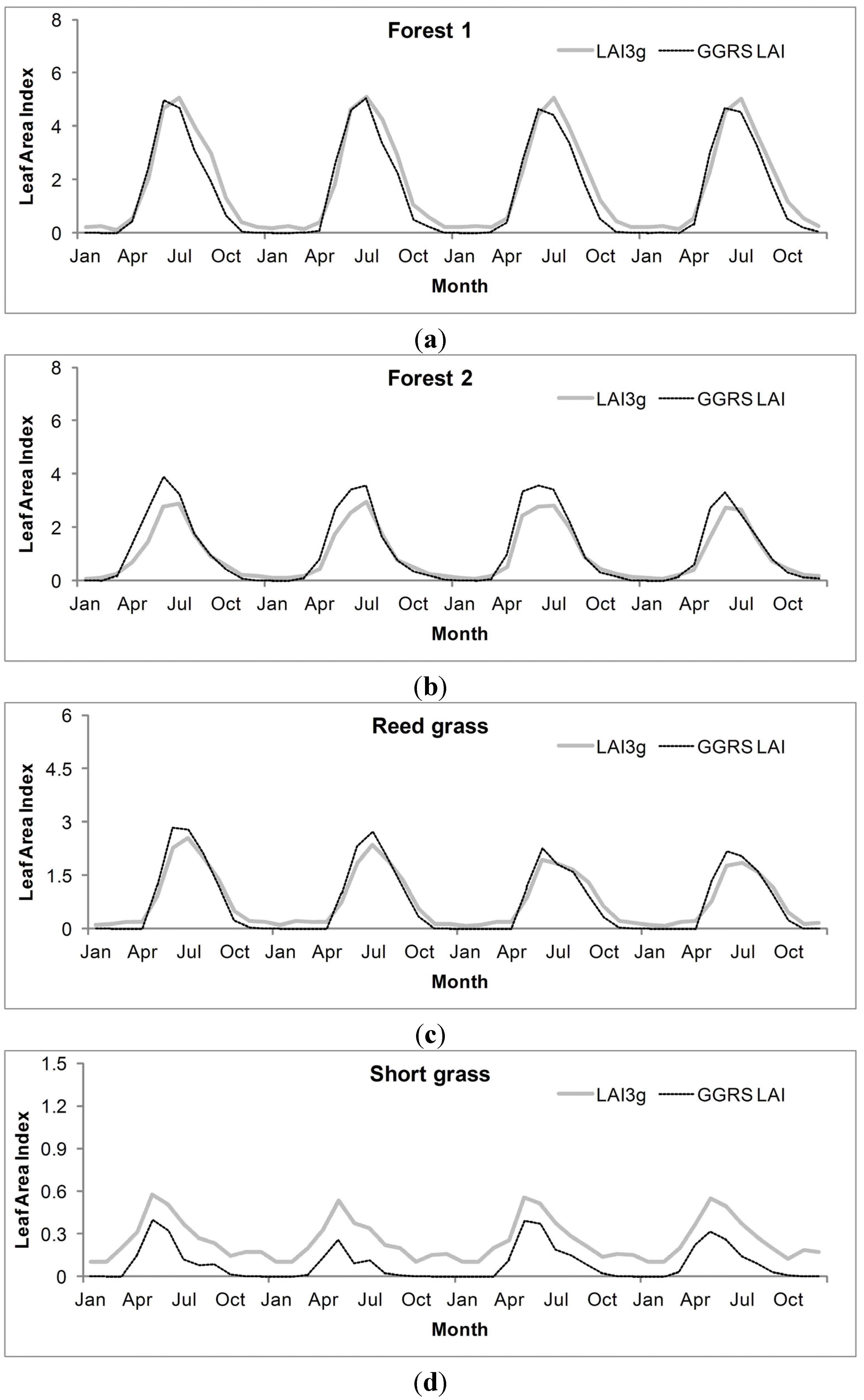
Temporal variations of LAI3g and LAI GGRS over the test sites with the main land cover types of Kazakhstan are compared in
Figure 9. The LAI data estimated for the representative test sites over Forest 1, Forest 2 and Reed Grass sites show consistent dynamics between LAI3g and LAI GGRS, but there are some differences in their temporal development. Thus, LAI3g in Forest 1 decreases in the leaf withering period (July–October) somewhat later than does LAI GGRS. For the Forest 2 and Reed Grass sites, the amplitude of LAI3g is much lower than that of LAI GGRS, due to lower values at the peak of the growing season and significantly higher values (LAI = 0.11–0.20) during the leafless phase (November–March).
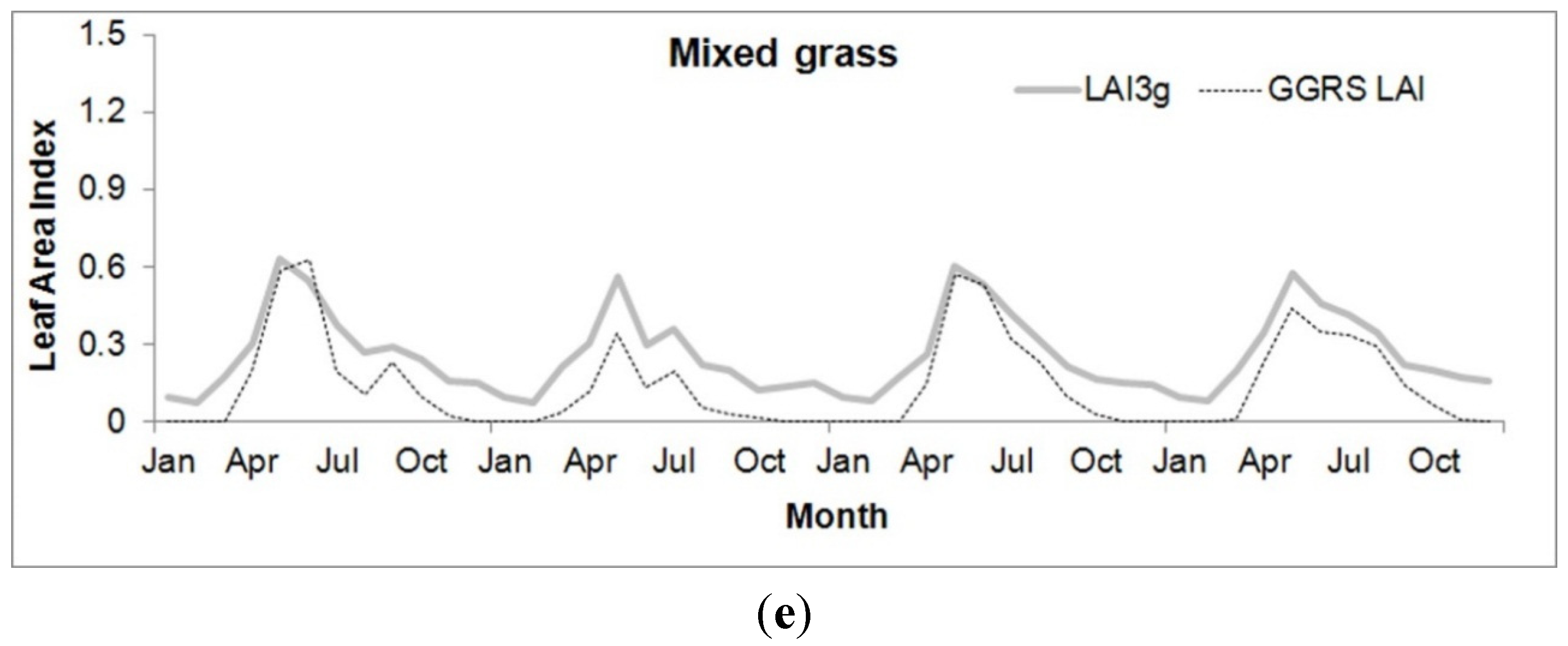
The test sites in short grassland and mixed grassland (
Figure 9d,e) have much less dynamic consistency between the datasets. Both the seasonal magnitude and the timing of the time series are characterized by distinct differences. For the short grass test site, the LAI3g product shows much higher values during the whole vegetation growth period. The typical LAI values for short grassland in the area around the test site are 0.25–0.40 from field observations [
19]. The LAI3g retrievals for short grassland are considerably higher. For the mixed grass test site, LAI values at the peak of the growing season are to some extent consistent between both datasets. However, LAI values during the senescence and autumn withering periods are different. During the leafless period, the LAI3g retrievals at the short and mixed grass test sites show LAI values significantly greater than zero (0.1–0.2), while LAI GGRS does not.
Within the study area, the principal mode of vegetation variability is generally associated with intra-annual seasonality of green leaf area. The seasonality in LAI of temperate climate zones is caused by a seasonal increase/decrease in solar radiation and air temperature, which serves as a proximate signal for the start/stop of leaf production. During the period November–March, when the temperature in the study area is below 0 °C, no vegetation activity is possible. The graphs in
Figure 9 demonstrate that the LAI3g product tends to ignore the annual dynamics of air temperature over Kazakhstan. The LAI3g product has values above zero for months outside the growing season. A recent publication [
26] has also noticed stronger differences between the various datasets at the start/end of the growing season. Further investigations, also using time series of
in situ LAI measurements in the leafless period, are needed to better understand the causes of the observed disagreement and to draw conclusions.
Figure 9.
Seasonal trajectories of LAI3g and LAI GGRS for test sites in forest (a,b); reed grass (c); short grass (d); and mixed grass (e) during the period 2005–2008.
Figure 9.
Seasonal trajectories of LAI3g and LAI GGRS for test sites in forest (a,b); reed grass (c); short grass (d); and mixed grass (e) during the period 2005–2008.


