Automatic Boat Identification System for VIIRS Low Light Imaging Data

Abstract

The ability for satellite sensors to detect lit fishing boats has been known since the 1970s. However, the use of the observations has been limited by the lack of an automatic algorithm for reporting the location and brightness of offshore lighting features arising from boats. An examination of lit fishing boat features in Visible Infrared Imaging Radiometer Suite (VIIRS) day/night band (DNB) data indicates that the features are essentially spikes. We have developed a set of algorithms for automatic detection of spikes and characterization of the sharpness of spike features. A spike detection algorithm generates a list of candidate boat detections. A second algorithm measures the height of the spikes for the discard of ionospheric energetic particle detections and to rate boat detections as either strong or weak. A sharpness index is used to label boat detections that appear blurry due to the scattering of light by clouds. The candidate spikes are then filtered to remove features on land and gas flares. A validation study conducted using analyst selected boat detections found the automatic algorithm detected 99.3% of the reference pixel set. VIIRS boat detection data can provide fishery agencies with up-to-date information of fishing boat activity and changes in this activity in response to new regulations and enforcement regimes. The data can provide indications of illegal fishing activity in restricted areas and incursions across Exclusive Economic Zone (EEZ) boundaries. VIIRS boat detections occur widely offshore from East and Southeast Asia, South America and several other regions.

1. Introduction

It has been known since the 1970s that low light imaging sensors flown on satellites are capable of detecting heavily lit fishing boats at night [1,2]. In general, these are boats using lights to attract catch. A recent study [3] found that lights from other types of boats can also be detected by satellite sensors at night. There are several published studies documenting the value of these observations to fishery management [4,5,6,7,8,9,10]. Despite the long record of use, to date there has not been an automatic algorithm for extracting and reporting the detection of boats based on lights.

The first system capable of global monitoring of lit fishing boats was the U.S. Air Force Defense Meteorological Satellite Program (DMSP) Operational Linescan System (OLS). NOAA’s National Geophysical Data Center (NGDC) serves as the DMSP archive and source for DMSP data. In year 2000, NGDC was granted permission to distribute 3+ hour old OLS data. Following this change, NGDC established a series of data services, supplying nighttime OLS data to fishery agencies in Japan, Korea, Thailand, and Peru.

The successful launch of the Suomi National Polar Partnership (SNPP) satellite in 2011 marked the advent of a new era in the capability for satellite low light imaging [11,12,13,14]. The primary imager on SNPP is the Visible Infrared Imaging Radiometer Suite (VIIRS). The VIIRS day/night band (DNB) collects low light imaging data with 45 times smaller pixel footprint than the OLS [11]. The VIIRS has other advantages over the OLS in terms of a higher level of quantization, rigorous calibration, and additional spectral bands useful for cloud, ocean and combustion source characterization.

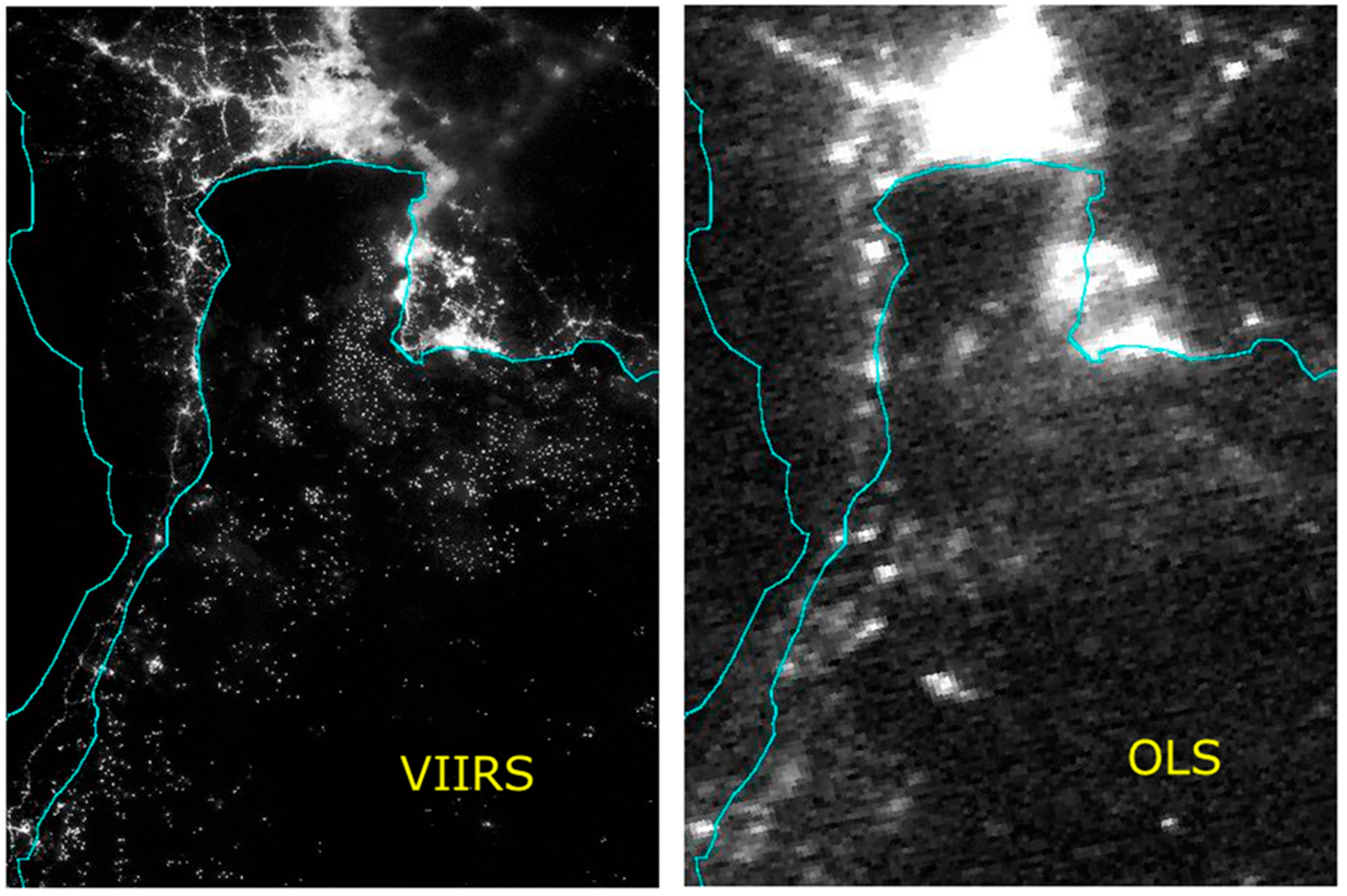
Figure 1. Visible Infrared Imaging Radiometer Suite (VIIRS) vs. Operational Linescan System (OLS) low light imaging data collected over Bangkok and the Gulf of Thailand region approximately five hours apart on the night of 14 October 2012. Note that the higher spatial resolution of the VIIRS data enables the detection of a vastly larger number of individual lighting features offshore.

Figure 1. Visible Infrared Imaging Radiometer Suite (VIIRS) vs. Operational Linescan System (OLS) low light imaging data collected over Bangkok and the Gulf of Thailand region approximately five hours apart on the night of 14 October 2012. Note that the higher spatial resolution of the VIIRS data enables the detection of a vastly larger number of individual lighting features offshore.

VIIRS is capable of detecting vastly more lit fishing boat features when compared to DMSP (Figure 1). However, the improvements in VIIRS over DMSP comes with a price—a vast increase in data volume. The basic data unit of VIIRS data is an “aggregate” spanning an area 3000 km wide and 2600 km high. The data volume for a DNB aggregate is 540 MB. The corresponding subset from a DMSP orbit tallies out to only 2.4 MB. Thus, the VIIRS data volume is 225 times higher than DMSP.

This data volume increase has emerged as a major obstacle for use of VIIRS fishing boat detections by fishery agencies and others organizations. There are very few organizations with the bandwidth and image processing capabilities to work with the source data. Expanding the user community for VIIRS boat detections is only feasible through a vast reduction in data volume. Recognizing this, we initiated the development of an automatic system for reporting locations of boats from VIIRS data. This paper describes key elements of the system.

2. Detection Algorithms

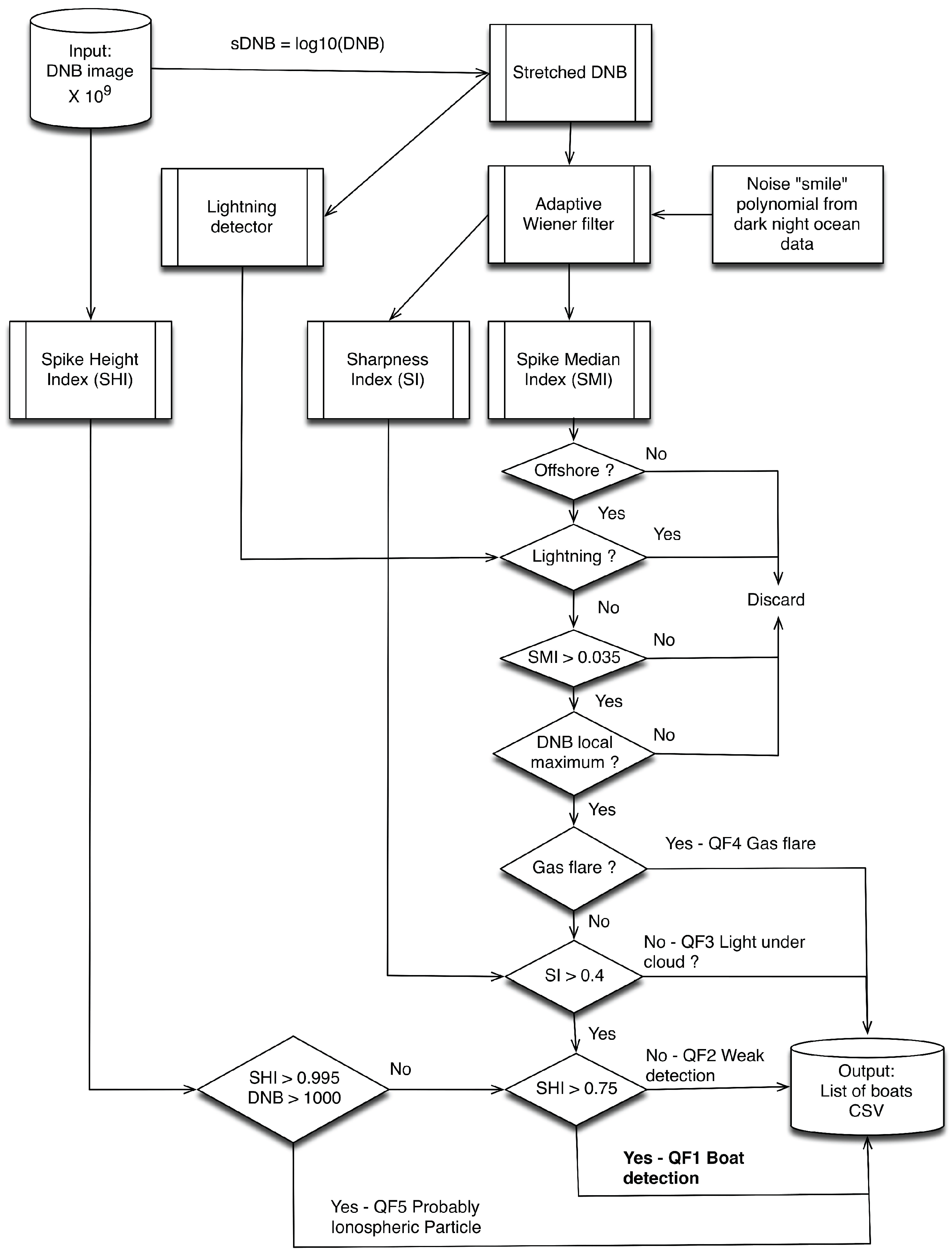
An examination of lit fishing boat features in VIIRS DNB data indicates that the features are essentially spikes. We have developed a set of algorithms for automatic detection of spikes and characterization of the sharpness of features (Figure 2). There is a spike detection algorithm that generates a list of spike features present in the DNB image data. A second algorithm rates the height of the spikes, which is used to discard energetic particle detections and rate boat detections as either strong or weak. A sharpness index is used to label boat detections that appear blurry due to the scattering of light by clouds. The spikes are then filtered to remove features on land and to label gas flares. Output records are written to comma-separated values (csv) files.

2.1. Pre-Processing

There are three pre-processing steps applied to the DNB data to prepare them for further analysis and use. The DNB data are produced in radiance units of Watts/cm²/sr/. The first pre-processing step is to multiply the DNB radiances by a billion (nanowatts). This is done to ease the human minds ability to read and understand the output data values. The original data values generally have seven to ten zeros after the decimal point before the start of significant digits. The large numbers of zeros make it difficult for the typical human to grasp. The solution is to multiply by a billion, which generally results in a number with one or two digits to the left of decimal point and a string of values to the right of the decimal point. The second pre-processing step is to enhance the contrast of features by taking the logarithm of the DNB radiances. These data are used as input to the lightning detector and after noise flattening, in the sharpness index and spike detection.

The third pre-processing step is to flatten noise levels across the swath using an adaptive Weiner filter [15]. At night, the DNB maintains a nearly constant pixel footprint of 742 m on a side, from nadir out to edge of scan. The pixel footprints of individual detectors will naturally expand from nadir to the edge of scan because of increased distance from the sensor to the earth’s surface. The pixel footprint is maintained at 742 m by aggregating different numbers of detectors. At nadir the DNB aggregates 66 detectors along scan and 42 detectors along track to form a single pixel out of 2772 total detectors. The number of detectors being aggregated gradually declines in 31 steps to each side of nadir, ending with pixel formed with 11 detectors along scan and 20 detectors along track (220 total detectors). The signal from the individual detectors is quite noisy. However, the noise from the individual detectors is suppressed by the aggregation. Signal to noise increases with the square root of the number of measurements that are averaged. Thus, the noise at the edge of scan is higher than at nadir, simply based on the number of detectors being aggregated. By flattening the noise across the swath it is possible to use a single threshold for identifying sharp lights and spikes.

Figure 2. Processing flow chart for VIIRS boat detection under low lunar illuminance conditions. The system detects and then assigns them to one of five categories using a quality flag. The highest quality detections are assigned to QF1. QF2 = weaker detections, QF3 = blurry detections, QF4 = gas flares, and QF5 = energetic particle detections.

Figure 2. Processing flow chart for VIIRS boat detection under low lunar illuminance conditions. The system detects and then assigns them to one of five categories using a quality flag. The highest quality detections are assigned to QF1. QF2 = weaker detections, QF3 = blurry detections, QF4 = gas flares, and QF5 = energetic particle detections.

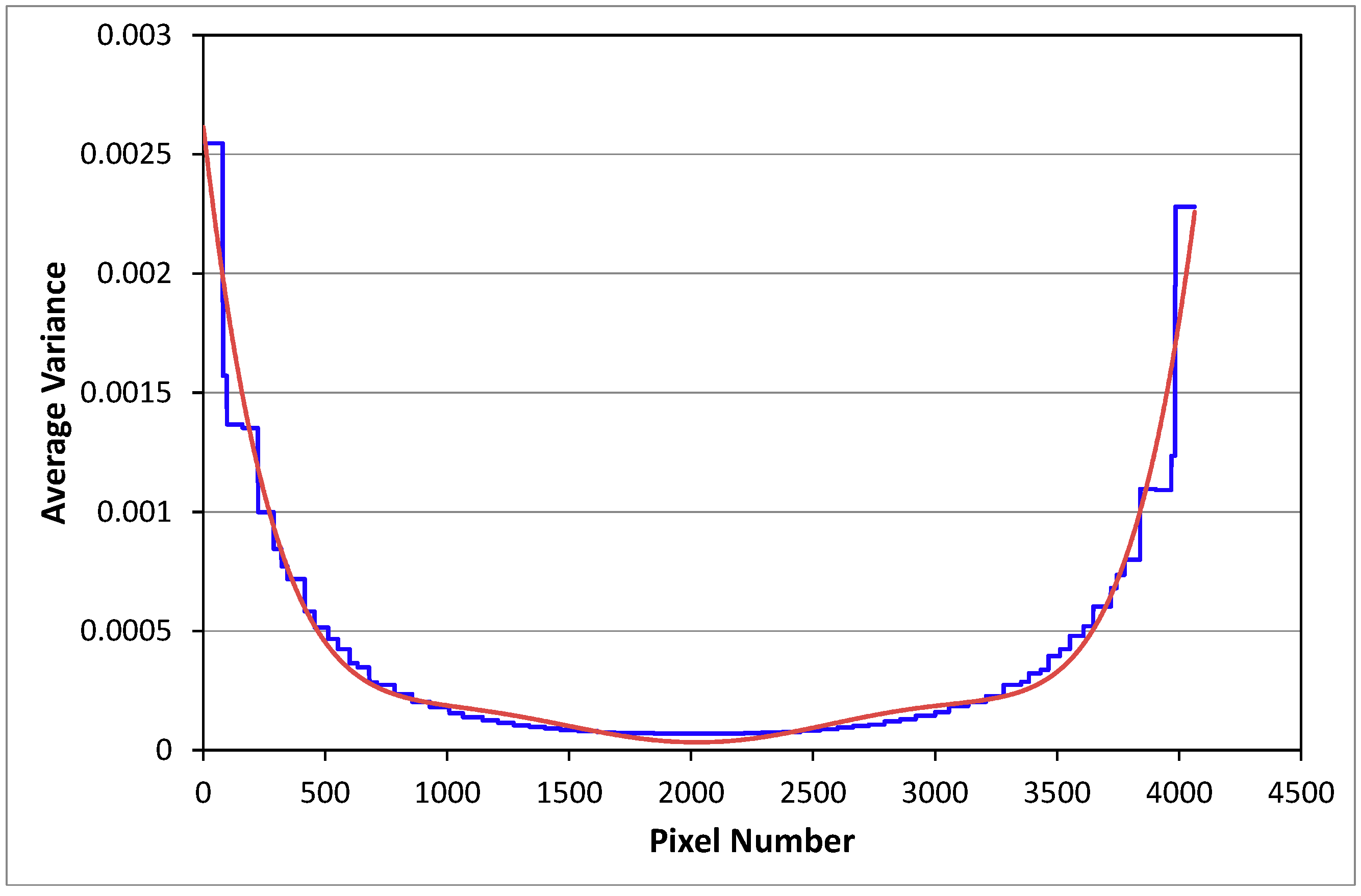
DNB data collected on moonless nights over deep ocean are used to characterize the scan angle dependency of white noise levels. The local variance is analyzed with 3 × 3 tiles and then average variance is derived for each aggregation zone. This is the blue line on Figure 3. The shape of the “smile” is summarized with a sixth order polynomial (the red line on Figure 3), which the Weiner filter uses to flatten noise levels across the image swath. The flattened data are used as input to the sharpness index and the spike detector.

Figure 3. The blue line indicates local variance for individual aggregation zones for the log(DNB) data from a reference dark night open ocean aggregate. This metric shows the increase in noise levels as a function of scan angle and aggregation zone and is sometimes referred to as “the smile”. The green line is a sixth order polynomial fit, which is used as input to the Weiner filter to flatten noise levels across the full swath.

Figure 3. The blue line indicates local variance for individual aggregation zones for the log(DNB) data from a reference dark night open ocean aggregate. This metric shows the increase in noise levels as a function of scan angle and aggregation zone and is sometimes referred to as “the smile”. The green line is a sixth order polynomial fit, which is used as input to the Weiner filter to flatten noise levels across the full swath.

2.2. Spike Detector

Under clear viewing conditions, lit fishing boats appear as individual spots of lighting in DNB data (Figure 1). In many cases, there are multiple spots, forming loose clusters in offshore locations. The spike detector operates on the Weiner filtered stretched DNB data. There are three steps in the spike detection algorithm:

(1)

Generation of a de-spiked version of DNB aggregate using a 3 × 3 median filter. Median filtering is a nonlinear operation often used in image processing to reduce “salt and pepper” noise [15]. The median filter considers each pixel in the image in turn and replaces the pixel value with the median of neighboring pixel values. The median is calculated by sorting all the pixel values from the surrounding 3 × 3 neighborhood into numerical order and then selecting the value in the fifth position. The median is more robust than the mean because a single unrepresentative pixel (e.g., spike) in a neighborhood will have minimal affect the median.

(2)

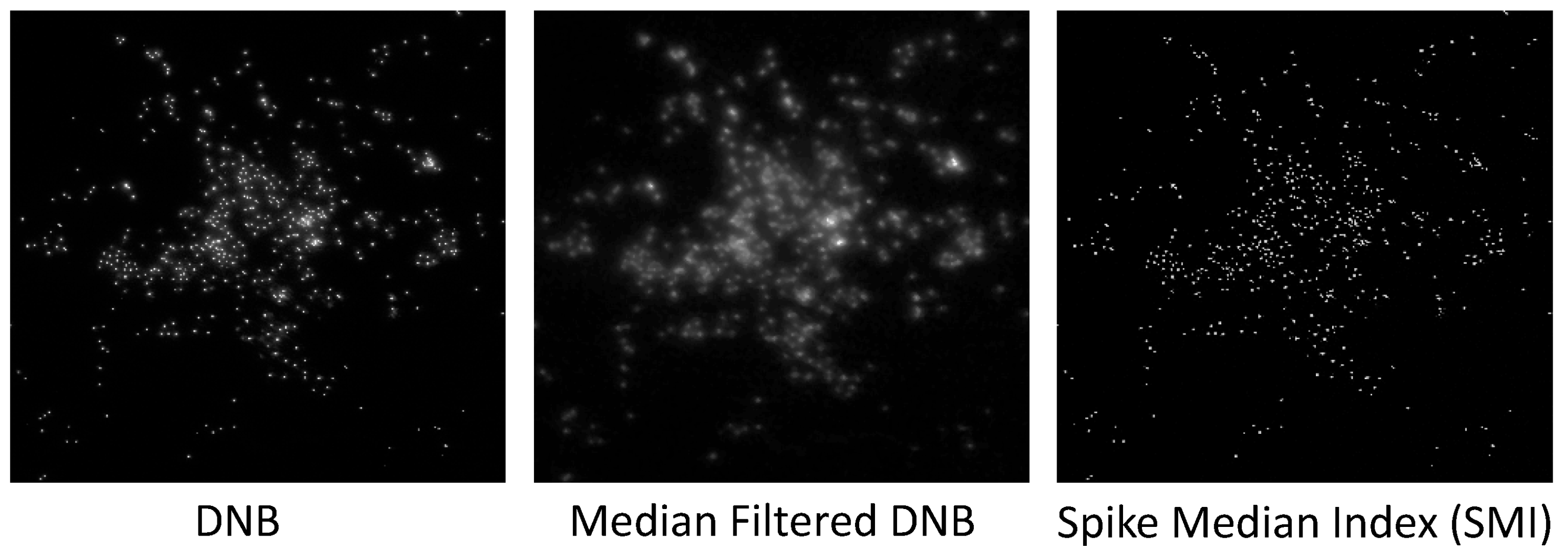
A spike median index (SMI) image is created by subtracting the median filtered image from original image (Figure 4).

(3)

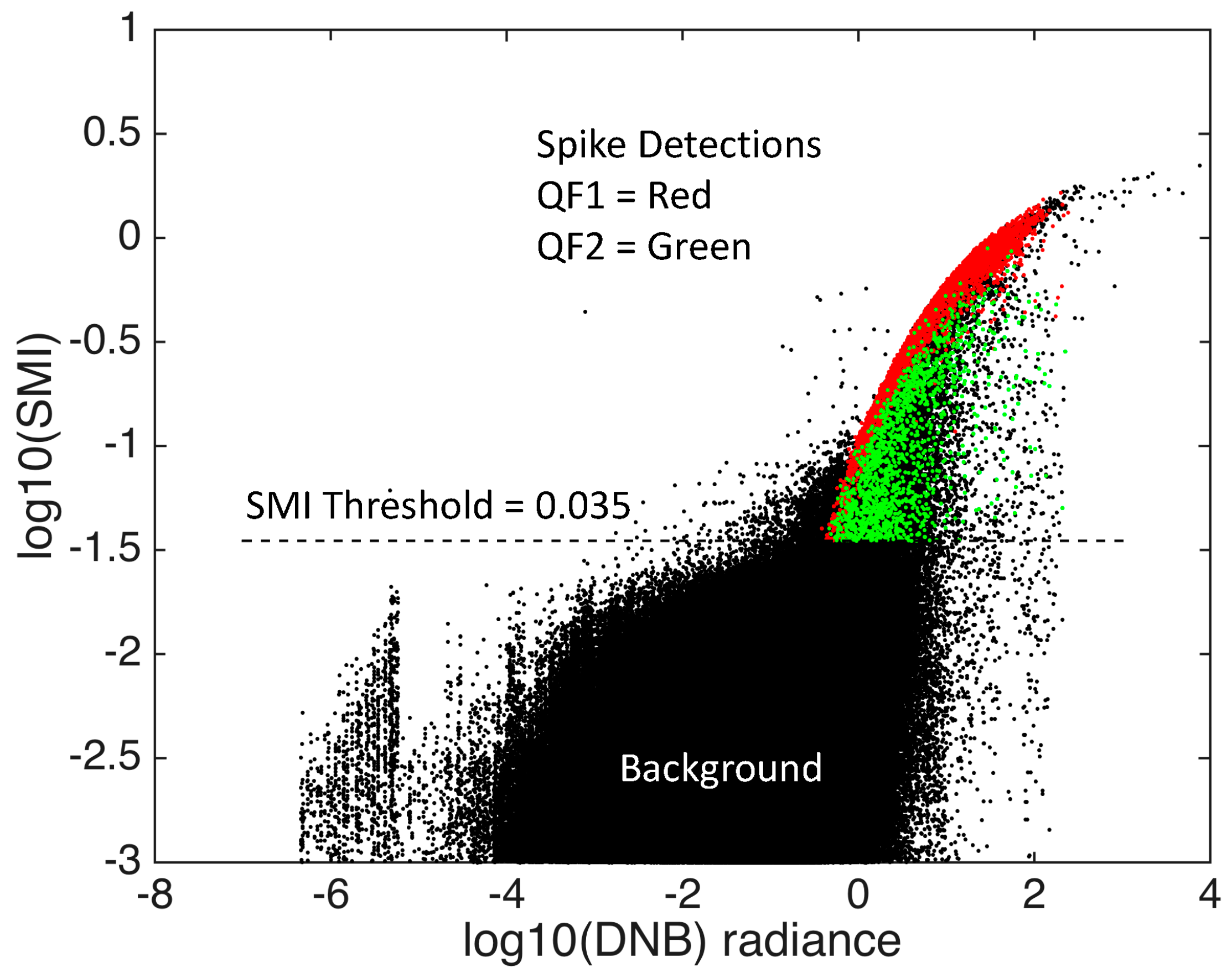
A threshold is applied is applied to the SMI image to identify the spikes. In developing the SMI detection threshold we first considered scattergrams of SMI values vs. DNB radiances from multiple aggregates (Figure 5). Background pixels have low radiance and low SMI values, forming a dense cloud of pixels in the lower part of the scattergram. Spikes form a quill-like extension at the top of the background data cloud. An analyst made an initial threshold selection based on the scattergram. The analyst then adjusted the threshold to minimize salt-and-pepper noise. After review of a large number of datasets, a threshold of 0.035 was selected for the detection of spikes with the SMI.

Figure 4. Example of raw DNB data, median filtered version with spike removed, and spike feature image made by subtracting the median filtered image from the original data.

Figure 4. Example of raw DNB data, median filtered version with spike removed, and spike feature image made by subtracting the median filtered image from the original data.

Figure 5. Scattergram of spike median index (SMI) vs. DNB radiances for a DNB aggregate. There is a dense cloud of background data values in the lower center part of the chart. Spike features are present in the quill-like appendage on the upper right side of the background pixel set. The red and green points are from QF1 (red) and QF2 (green) spike detections.

Figure 5. Scattergram of spike median index (SMI) vs. DNB radiances for a DNB aggregate. There is a dense cloud of background data values in the lower center part of the chart. Spike features are present in the quill-like appendage on the upper right side of the background pixel set. The red and green points are from QF1 (red) and QF2 (green) spike detections.

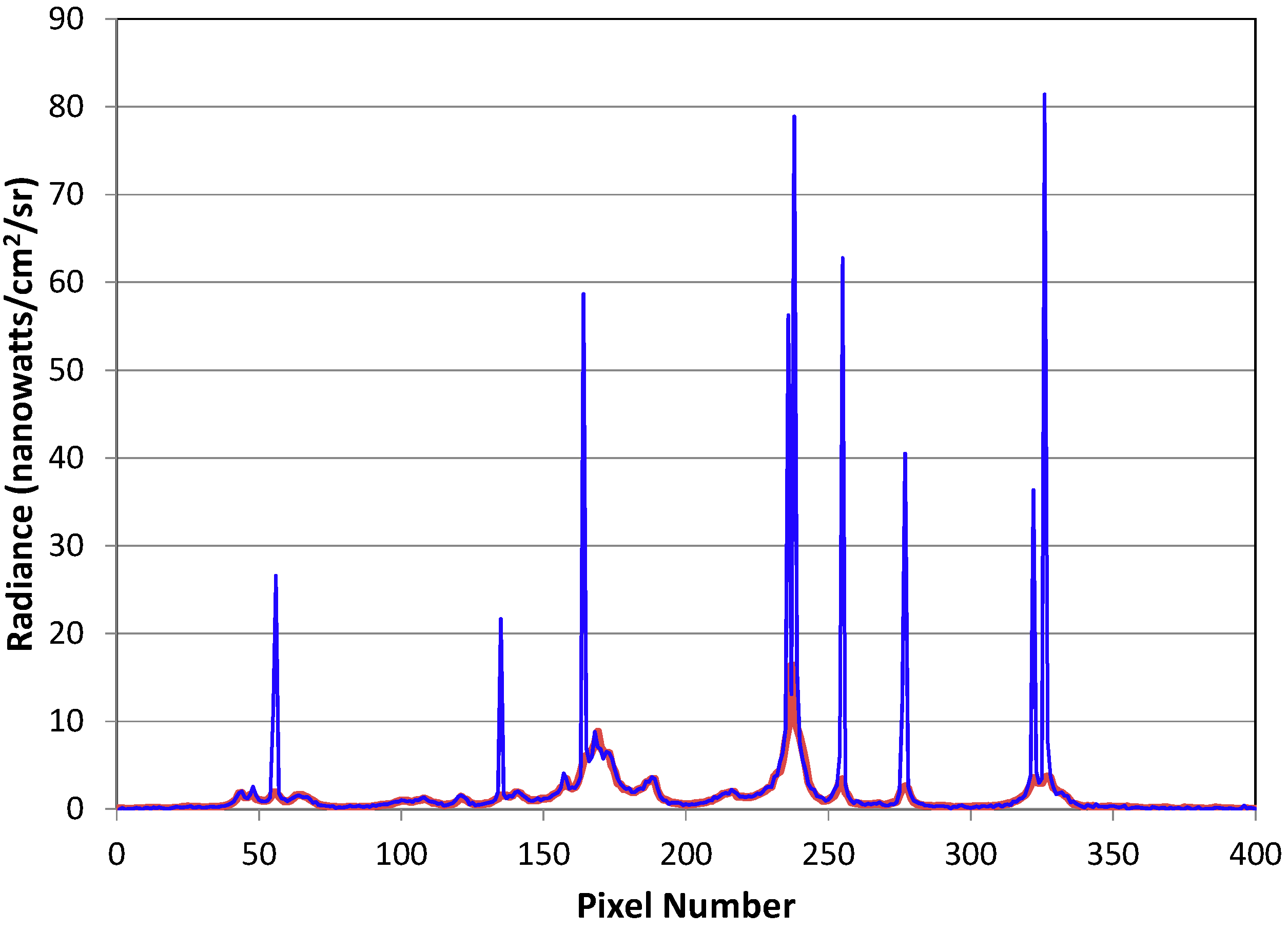
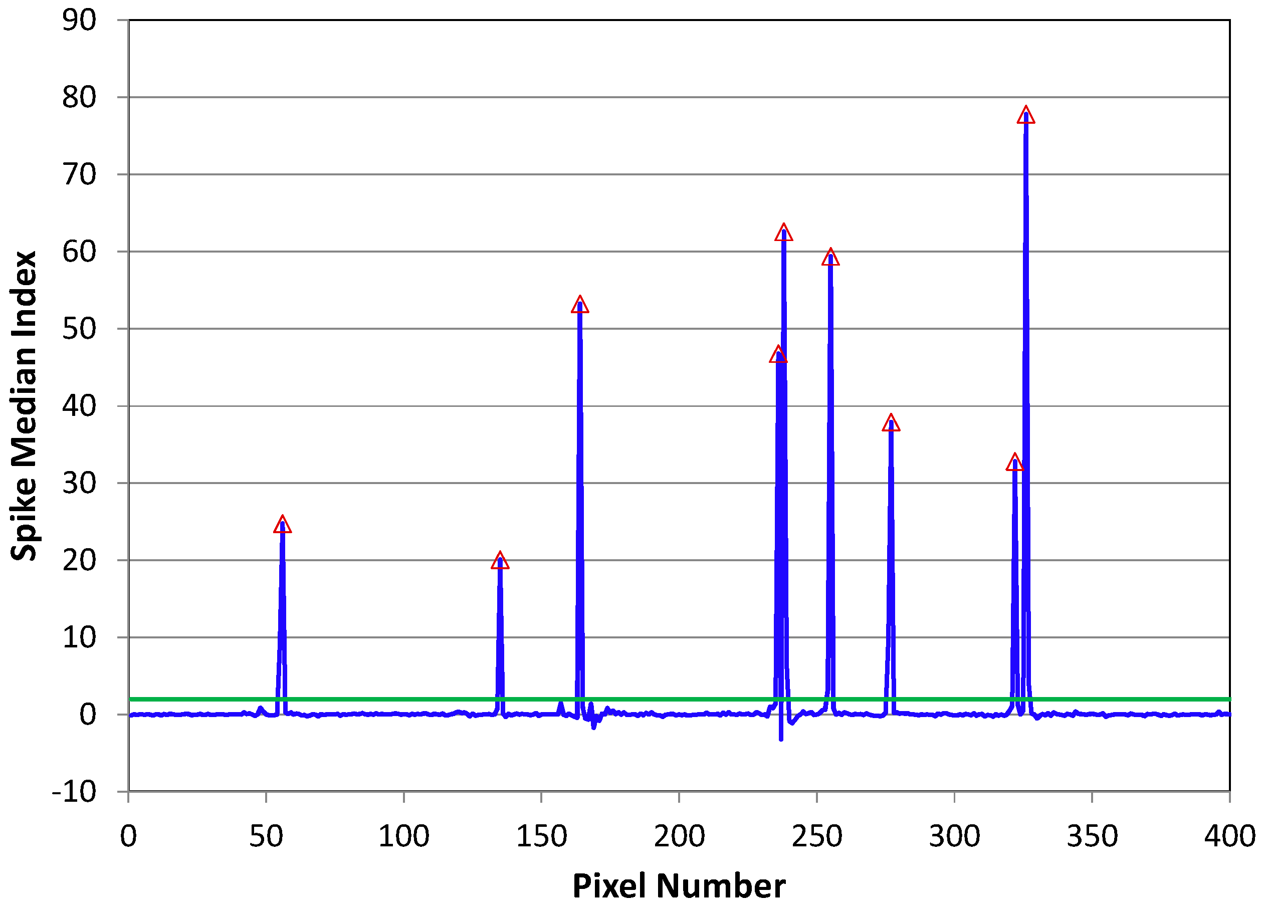
Figure 6 and Figure 7 show the operation of the spike detection algorithm for pixels along a transect across a cluster of boats. A threshold is applied to the SMI image to detect spikes. Only local maxima features are retained. Then the spike detections are rated with the processes described below to generate a list of boat detections based on their strength and sharpness. These ratings are recorded as with the assignment of a quality flag (QF) value. The highest quality detections are assigned to QF1. The other values are QF2 for weaker detections, QF3 for blurry detections, QF4 are gas flares, and QF5 are energetic particle detections.

Figure 6. Example transect of DNB data with boat detection spikes (blue) and the median filtered counterpart (red).

Figure 6. Example transect of DNB data with boat detection spikes (blue) and the median filtered counterpart (red).

Figure 7. Spike Median Index (SMI) data of the transect from Figure 6. The green line is the detection threshold. The red triangles mark the location of detected spikes.

Figure 7. Spike Median Index (SMI) data of the transect from Figure 6. The green line is the detection threshold. The red triangles mark the location of detected spikes.

2.3. Spike Height Index (SHI)

The SHI has two functions. It is used to label false DNB detections arising from energetic particle impacts on detectors. Secondly, the SHI is used to divide the sharp boat detections into two categories: strong and weak. The DNB records extremely high radiance values when high energy particles present in the ionosphere impact on individual detectors. These are most prevalent in the South Atlantic Anomaly, a well-known disturbance in the Earth’s ionosphere [16]. The noise hits also occur when the spacecraft flies through auroral zones. It is important to recognize and discard these ionospheric noise detections as part of the boat analysis. The spike height index (SHI) is calculated as the ratio between the spike’s radiance and the average radiance of the adjacent pixels. In addition to detection ionospheric noise, the SHI is used to confirm the pixels identified by the spike detector.

$$SHI=\frac{(radiance of the subject pixel-average radiance of the two adjacent pixels)}{radiance of the subject pixel}$$

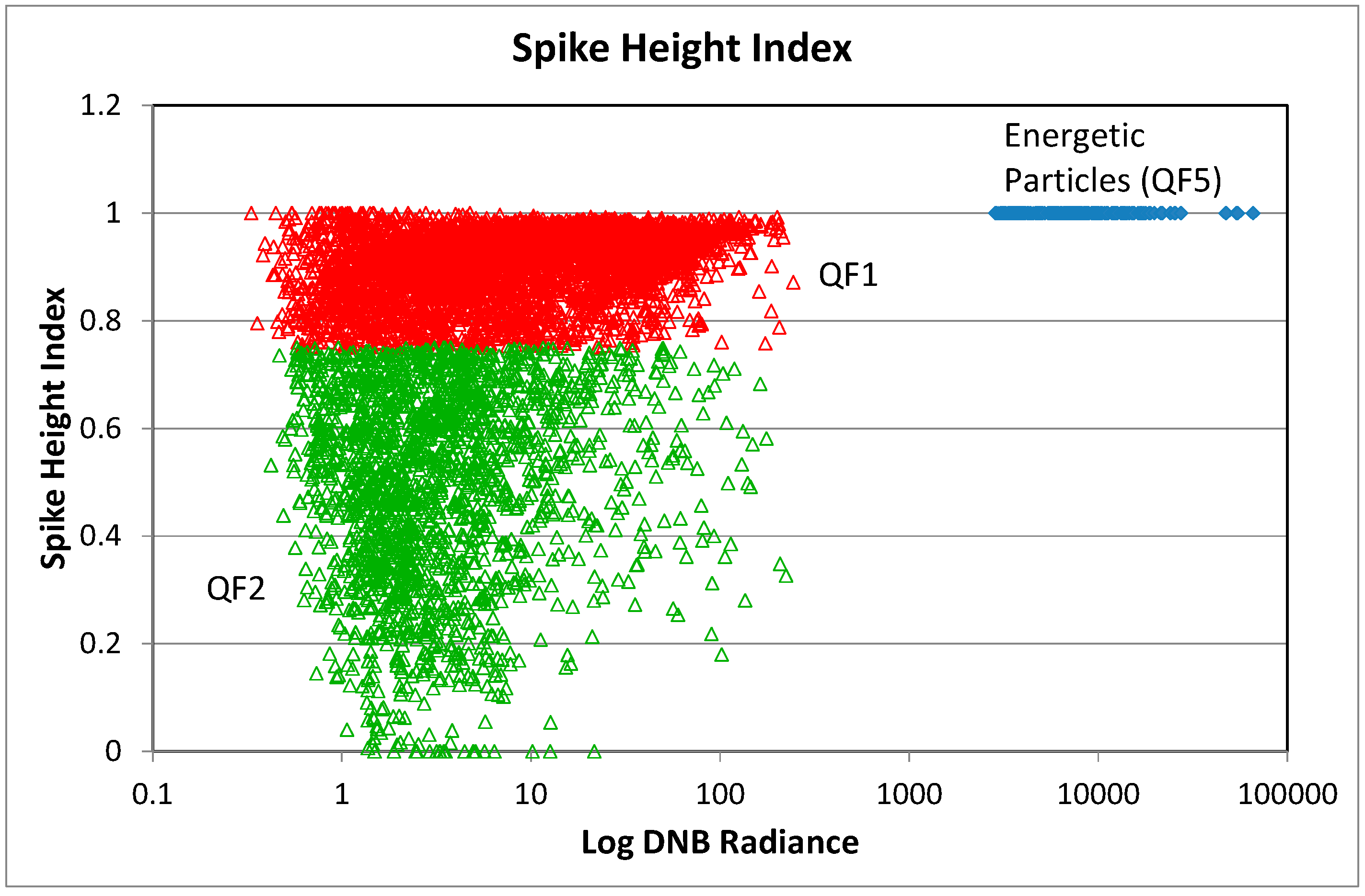
The SHI is run on each pixel in the image horizontally along lines and vertically along columns. Along lines, the adjacent pixels are the two pixels to either side (left and right) of the subject pixel. Along columns, the adjacent pixels are pixel above and pixel below the subject pixel. This results in two height measures, horizontal and vertical. Thresholds are set on the smaller of the two. Pixels with spike height index values in excess of 0.995 and radiance values exceed 1000 nanowatts are labeled as ionospheric noise and are recorded as QF5 (Figure 8). The SHI values for are used to rate spike detections from the primary spike detection algorithm as either strong or weak. Strong detections with SHI > 0.75 are assigned a QF value of 1. Weak detections (SHI < 0.75) are assigned QF values of 2.

Figure 8. SHI vs. DNB radiances for three categories of pixels. Energetic particle detections have radiances exceeding 1000 nanowatts and SHI values in excess of 0.995. The SHI is used to divide the offshore lights into strong detections (QF1) and weak detections (QF2).

Figure 8. SHI vs. DNB radiances for three categories of pixels. Energetic particle detections have radiances exceeding 1000 nanowatts and SHI values in excess of 0.995. The SHI is used to divide the offshore lights into strong detections (QF1) and weak detections (QF2).

2.4. Sharpness Index

Each DNB image is analyzed with an algorithm that rates the sharpness of features. The objective is to identify detections that are impacted by clouds. After testing several blur detection options we settled on the S3 Spectral Measure of Sharpness algorithm [17]. S3 is based on a spectral measure of the slope of the local spatial spectrum of the image magnitude. The magnitude spectrum M(f) is known to fall inversely with spatial frequency, i.e., M(f)α f−α, where f is frequency and −α is the slope of the regression line log M α −α log f. An increase in α indicates a reduction in high-frequency content, and thus a reduction in image sharpness.

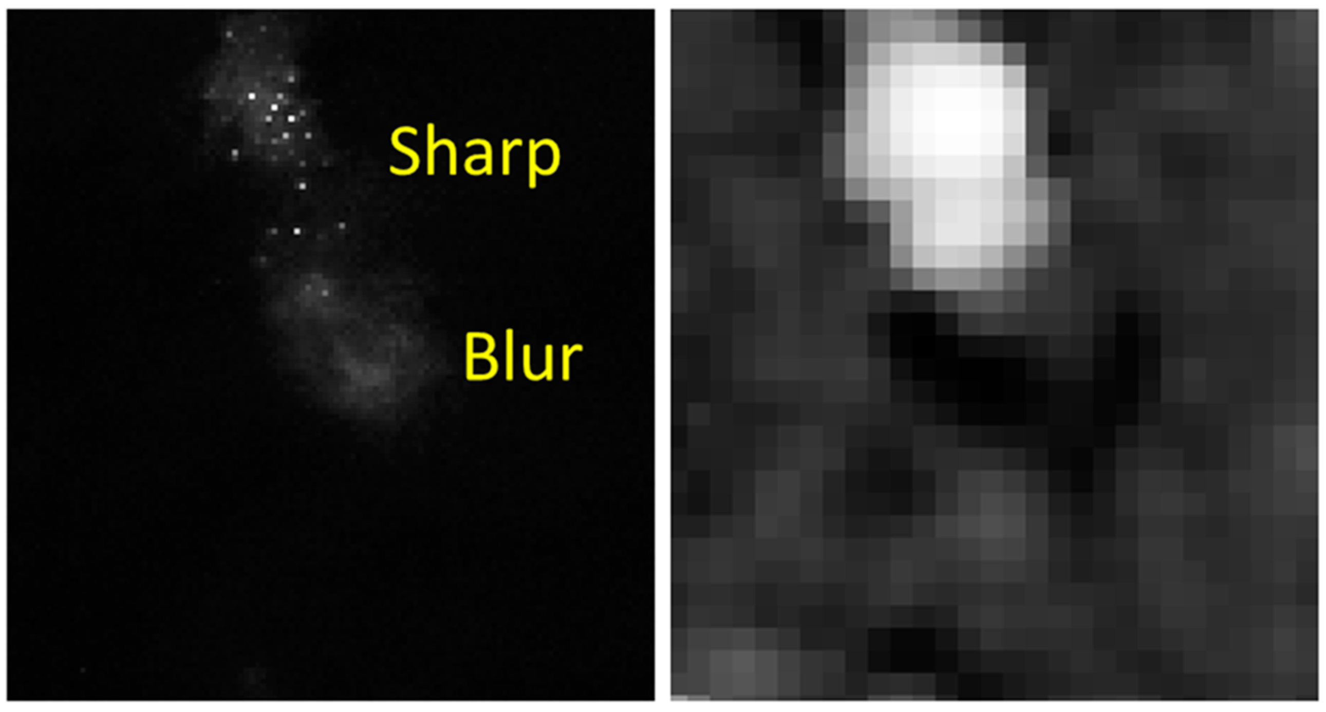
To rate the sharpness of the DNB features, the sharpness index S(α) is calculated for square blocks of size m = 32 and an overlap of d = 24. Figure 9 shows sharpness index values for a DNB image section containing a set of sharp lights and a blurred area. A threshold of 0.4 is used to distinguish between sharp and blurry SMI detections. Features with SI values greater than 0.4 are assigned to either QF1 or QF2 based on their SHI values. SMI detections with SI values under 0.4 are assigned to QF3 for blurry detections.

Figure 9. DNB for a set of sharp and fuzzy offshore lights vs. the corresponding blur detection output. Blur index values are high for sharp features and low for fuzzy features.

Figure 9. DNB for a set of sharp and fuzzy offshore lights vs. the corresponding blur detection output. Blur index values are high for sharp features and low for fuzzy features.

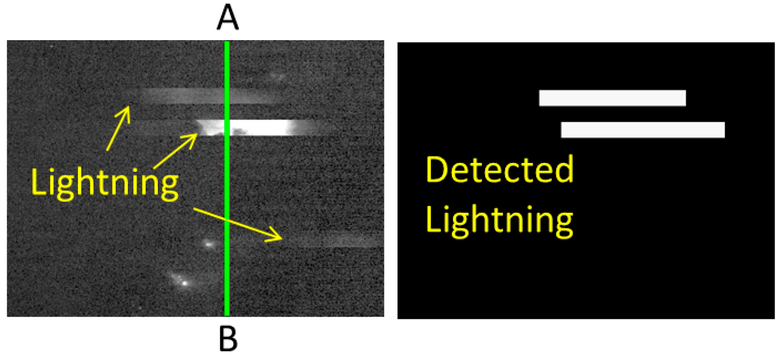
2.5. Lightning Detector

The DNB detects lightning as horizontal ribbons of lighting (Figure 10). These features are exactly 16 line wide, arising from the simultaneous collection of 16 lines of data in a single scan. The lighting detection algorithm is based on the detection of spatially extensive brightness steps along the boundaries between scans. The input files are the preprocessed DNB images described in Section 2.1 above. The procedure is outlined graphically in Figure 11.

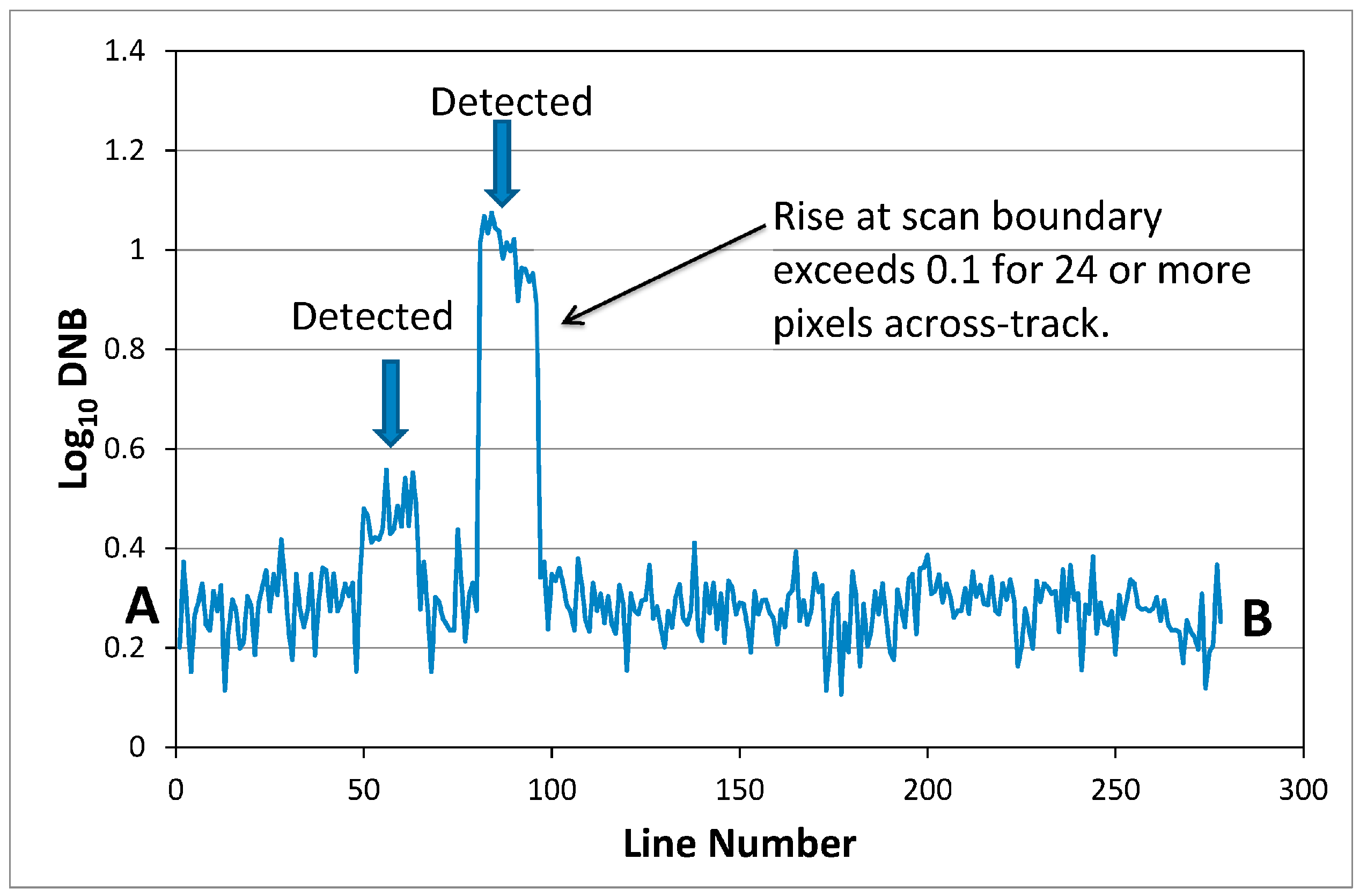
The lightning detection algorithm calculates radiance differences between scanlines separating the 16 line scans. Scan segments with differences greater than 0.1 Log10 DNB that persist for 24 or more consecutive pixels are labeled as lightning. Pixels labeled as lightning are discarded and not recorded in the output csv.

Figure 10. Illumination detected from lightning forms horizontal ribbons exactly 16 lines wide, corresponding to the number of lines collected in a single sensor scan. The sample images shows three lightning features. The A-B lines shows the position of the along-track transect presented in Figure 11. The algorithm detected two of the three lightning features.

Figure 10. Illumination detected from lightning forms horizontal ribbons exactly 16 lines wide, corresponding to the number of lines collected in a single sensor scan. The sample images shows three lightning features. The A-B lines shows the position of the along-track transect presented in Figure 11. The algorithm detected two of the three lightning features.

Figure 11. Graphical representation of the lightning algorithm based on the pixels along transect A–B on Figure 10.

Figure 11. Graphical representation of the lightning algorithm based on the pixels along transect A–B on Figure 10.

2.6. Masking to Offshore Areas

Each of the detected spikes is tested to determine if it is on land, near-shore or offshore. The land set is defined by the land-sea mask surrounded by a one km buffer. The near-shore detection set fall within 2 km of the land set. All other detections are labeled as offshore.

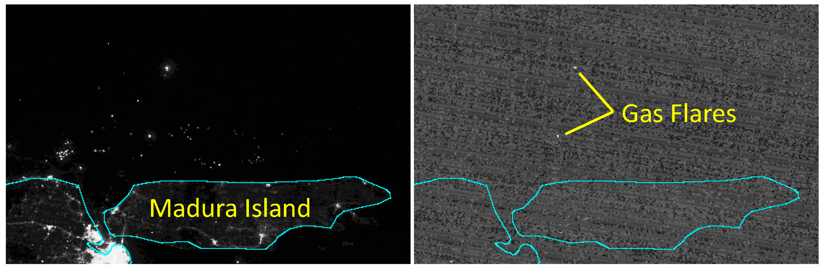
2.7. Filtering to Remove Gas Flares

The DNB spikes are checked to assign a QF value of 4 to those that are associated with gas flares. DNB spikes are labeled as gas flares if they are collocated with VIIRS band M10 combustion source detections [18]. The spikes are also compared to an annual database of known gas flares to ensure that all DNB spikes associated with gas flares are removed. Figure 12 shows an example of a series of offshore lights present in DNB data collected north of Madura Island, Indonesia. The only feature detected in the M10 data is the methane combustion from the gas flare. None of the lighting features are detected in M10.

Figure 12. The lighting features observed in DNB data collected north of Madura Island, Indonesia contains a combination of boats and gas flares. The two gas flares are identified based on short-wave infrared radiant emissions present in the simultaneously acquired M10 data.

Figure 12. The lighting features observed in DNB data collected north of Madura Island, Indonesia contains a combination of boats and gas flares. The two gas flares are identified based on short-wave infrared radiant emissions present in the simultaneously acquired M10 data.

3. Results

3.1. Nightly Results

Three styles of output are produced on a nightly basis:

(1)

CSV file (comma-separated values) recording date, time, latitude/longitude, DNB radiance, spike index, spike height index, and sharpness index values. Each detection has a quality flag rating: QF1 = strong detections, QF2 = weak detections, QF3 = blurry detections, QF4 = gas flares, and QF5 = energetic particles.

(2)

Kml and kmz of the boat detections for review in Google Earth.

(3)

A contrast enhanced DNB image with kml and kmz links for use in Google Earth. This provides context for interpreting the detections.

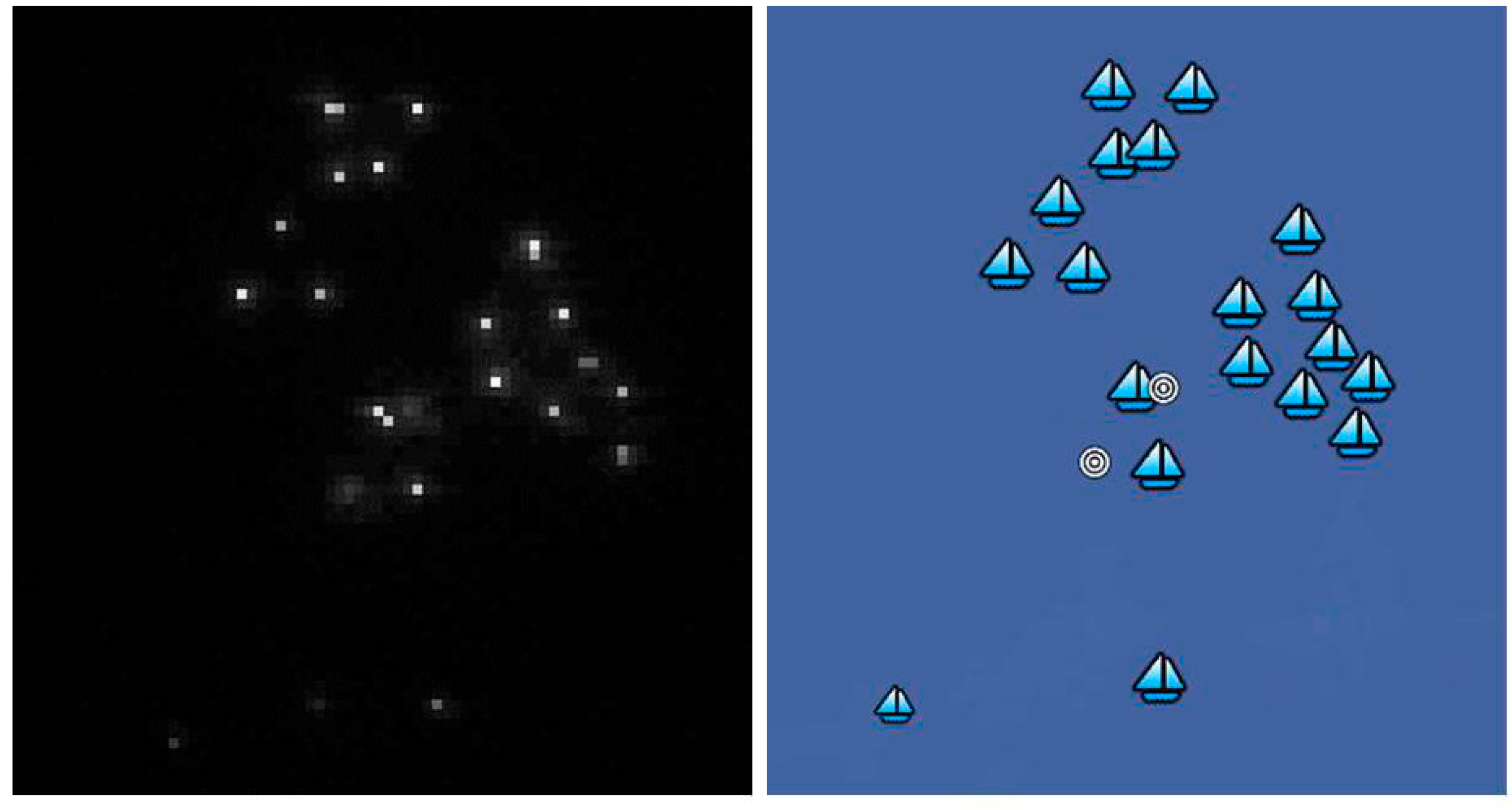
Nightly results are posted at an open access web site. The kmz placemarks are coded by detection type. Boats (QF1) in open water are represented by a sailing ship. These are sized based on the DNB radiance. Detections rated as blurry (QF3) by the sharpness index are marked with a storm cloud icon. Weak detections (QF2) are marked with three concentric circles. Gas flares (QF4) are marked with red balloons. Examination of the detections on top of the contrast enhanced DNB images indicate that the algorithm is working well on nights with low lunar illuminance (Figure 13).

Figure 13. The contrast enhanced DNB image subset on the left showing a cluster of boats. The corresponding boat detections are shown on the right. QF1 strong detections are marked as sailing boats. QF2 weak detections are marked as three concentric circles.

Figure 13. The contrast enhanced DNB image subset on the left showing a cluster of boats. The corresponding boat detections are shown on the right. QF1 strong detections are marked as sailing boats. QF2 weak detections are marked as three concentric circles.

3.2. Monthly Summaries

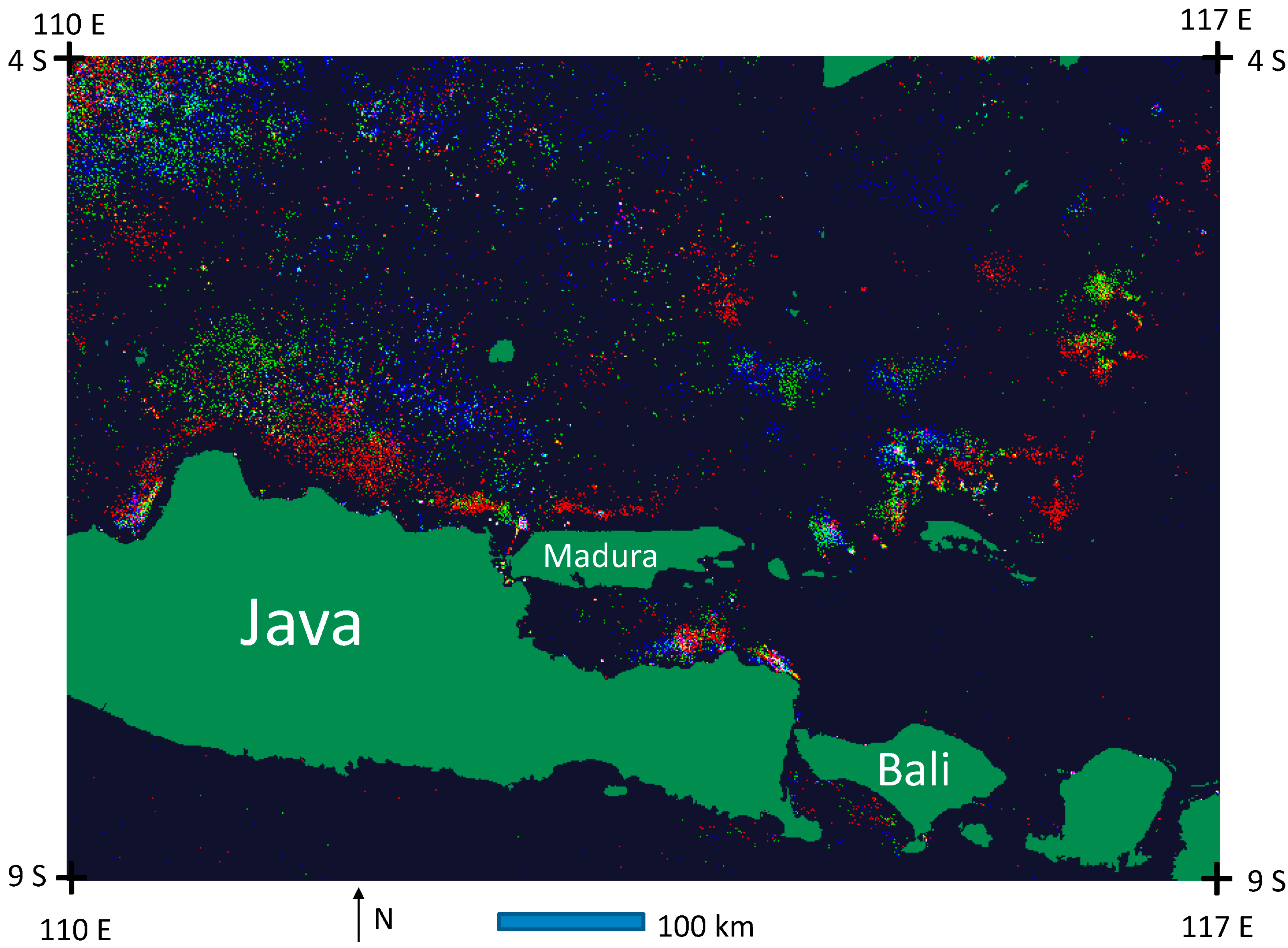
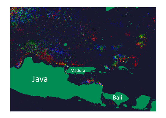
It is possible to summarize the results over monthly increments. This makes it possible to define fishing grounds and analyze the temporal dynamics of the fishing boat activity. Figure 14 shows three months of data for the East Java Sea, near the city of Surabaya. In this image the lights detected in October 2014 are red, September 2014 green, and August 2014 blue. There are three primary spatial patterns: (1) Diffused, with lights spaced out covering a large area. This can be seen in the western half of the image. (2) Dense clusters, seen in the eastern half of the image. In addition, (3) Stationary, these may be fishing platforms or storage boats parked at a single site for extended periods of time. The presence of colors in the image indicates that the fishing grounds are shifting spatially over time.

Figure 14. Color composite image of monthly boat detection activity in the Java Sea. October 2014 boat detections are red. September 2014 boat detections are green, August 2014 boat detections are blue. Other colors are formed when boats were detected in the same areas for two out of the three months. White indicates that boats (or platforms) were detected in all three months.

Figure 14. Color composite image of monthly boat detection activity in the Java Sea. October 2014 boat detections are red. September 2014 boat detections are green, August 2014 boat detections are blue. Other colors are formed when boats were detected in the same areas for two out of the three months. White indicates that boats (or platforms) were detected in all three months.

3.3. Validation

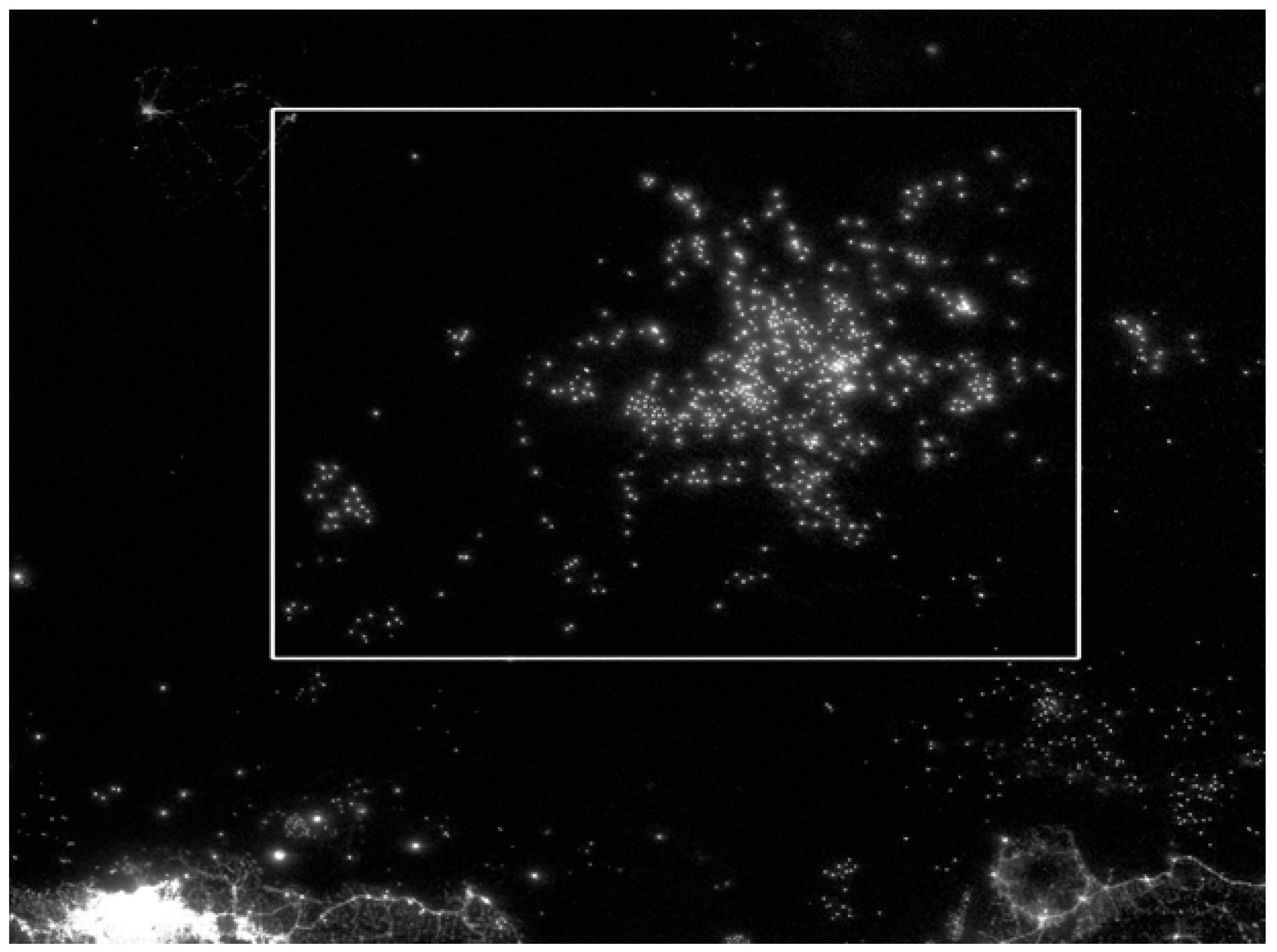
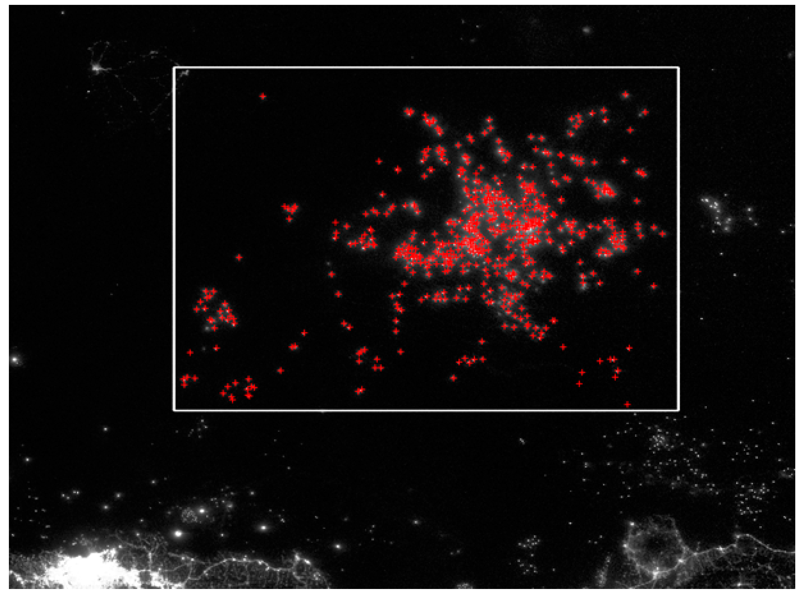
A validation was conducted to compare the algorithm results against boat detections made visually by an analyst using DNB data collected on a moonless night—27 September 2014. The analyst first defined a data collection box, marked by the rectangle on Figure 15. The analyst adjusted the contrast to enable visual identification of local maxima for the brightest boats. 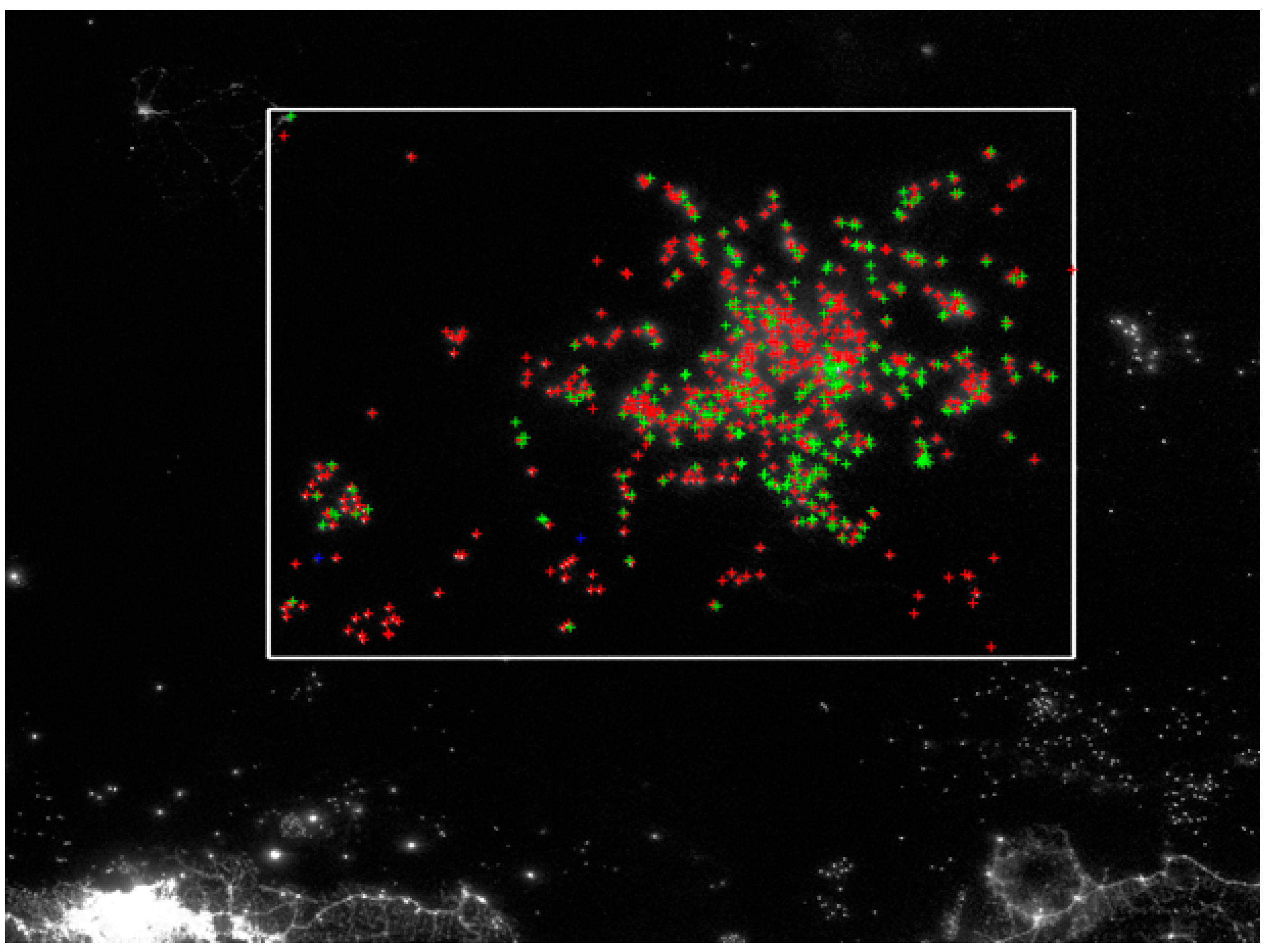Then the analyst manually moved the screen cursor to pixel locations identified as boats, creating a vector points for each (Figure 16). The analyst selected a total of 594 boat detection pixels. Then the standard algorithm was run and the results (Figure 17) were compared to the selections made by the analyst.

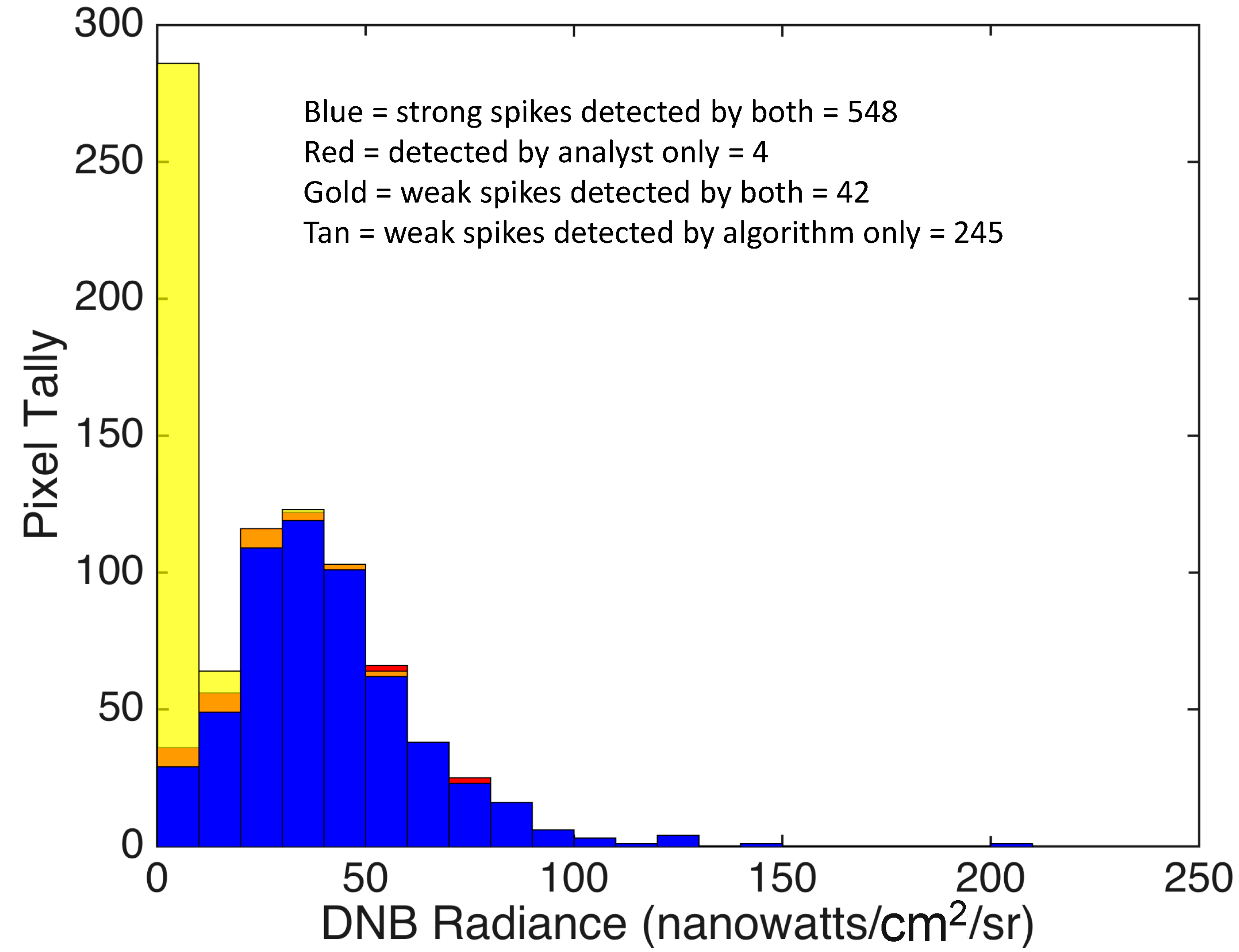
The algorithm detected 590 out of 594 boats identified by the analyst (Figure 18). The four non-detected boats are adjacent to local maxima that were detected by the algorithm. The four went un-detected because the current algorithm only reports detections for local maxima. The analyst and algorithm are in complete agreement on the QF1 boats. The analyst did well in detecting QF2 features for radiances above 20 nanowatts. The algorithm detected 245 QF2 pixels that were not selected by the analyst. Only two QF3 detections are present, neither of which are in the analyst selected boat detections.

Figure 15. DNB image of the Java Sea from 27 September 2014. The validation study area is marked with a white rectangle.

Figure 15. DNB image of the Java Sea from 27 September 2014. The validation study area is marked with a white rectangle.

Figure 16. The analysts identified 594 boats in the study area.

Figure 16. The analysts identified 594 boats in the study area.

Figure 17. Algorithm identified 835 features. Red = QF1 (458 detections), Green = QF2 (287 detections), Blue = QF3 (2 detections).

Figure 17. Algorithm identified 835 features. Red = QF1 (458 detections), Green = QF2 (287 detections), Blue = QF3 (2 detections).

Figure 18. Summary of the validation results.

Figure 18. Summary of the validation results.

4. Conclusions

A boat detection system has been developed for VIIRS DNB data. The system is fully automated and output files are typically available approximately four hours after the collections. Outputs include csv and kmz listing date, time, latitude, longitude, and DNB radiance. The quality of the detections are rated with three quality flag categorizations: QF1 = highest quality detections, QF2 = weaker detections, and QF3 = blurry detections. On a new moon night in Indonesia the system typically detects 5000–6000 boats per night.

The data have known limitations based on the sensor characteristics. The VIIRS DNB spectral bandpass spans 0.5 to 0.9 µm, straddling the visible and near infrared. With only a single band, it is not possible to distinguish different types of lighting, for example LED vs. incandescent [19]. The spatial footprint of the DNB is large enough that several boats could be present in a single pixel. A validation effort would be required to define the types of boats that are detected in terms of the installed wattage of lighting, lighting types, shielding present on the lights and orientation of the lights while in operation.

The system works well when lunar illuminance is low. Under full moon conditions the current algorithms produce large numbers of false detection arising from brightness variations in clouds. Additional algorithm development will be required to obtain reliable boat detections with minimal false detects under full moon conditions. It may be possible to automate the correlation of moonlit features in the DNB with correspond features from VIIRS long-wave infrared image data, enhancing the detectability of lighting features in the DNB.

While the data are unable to discern the ownership of a boat, there are several ways the data can be used to improve fishery management and combat IUU fishing (illegal, unregulated, unreported). VIIRS boat detections can be cross referenced with boat location data from VMS (vessel monitoring system) or AIS (automatic identification system) to identify boats that are not operating a location beacon. The boat detections can be overlain with outlines of Marine Protected Areas or seasonally restricted fishing grounds to identify illegal fishing. The detection data may be used to identify possible incursions of foreign fishing boats across EEZ lines. It may be possible to identify boats that are exceeding wattage limits placed on lighting. Monthly summary data can be used to track spatial and temporal shifts in fishing grounds and to identify stationary boats that may be storage boats collecting catch from a cadre of fishing boats. Finally, the data can be used by government agencies to target enforcement efforts and inspections to areas with concentrated fishing boat activity.

During the coming months NOAA plans to conduct a validation effort to better understand the types of boats and platforms that are detected and to analyze detection limits. Review of the VIIRS nighttime data indicate that boats are detected offshore in many locations in East and Southeast Asia, Australia, New Zealand, Peru, Ecuador, Argentina, and United Arab Emirates.

References

- Croft, T.A. Nighttime Images of the Earth from Space. Sci. Am. 1978, 239, 86–98. [Google Scholar] [CrossRef]
- Croft, T.A.; Colvocoresses, A.P. The Brightness of Lights on Earth at Night, Digitally Recorded by DMSP Satellite; USGS Open File Report; Series Number: 80-167; U.S. Geological Survey: Reston, VA, USA, 1979.
- Straka, W.C., III; Seaman, C.J.; Baugh, K.; Cole, K.; Stevens, E.; Miller, S.D. Utilization of the Suomi National Polar-Orbiting Partnership (NPP) Visible Infrared Imaging Radiometer Suite (VIIRS) day/night band for Arctic ship tracking and fisheries management. Remote Sens. 2015, 7, 971–989. [Google Scholar] [CrossRef]
- Cho, K.; Ito, R.; Shimoda, H.; Sakata, T. Fishing fleet lights and sea surface temperature distribution observed by DMSP/OLS sensor. Int. J. Remote Sens. 1999, 20, 3–9. [Google Scholar] [CrossRef]
- Rodhouse, P.G.; Elvidge, C.D.; Trathan, P.N. Remote sensing of the global light-fishing fleet: An analysis of interactions with oceanography, other fisheries and predators. Adv. Mar. Biol. 2001, 39, 261–303. [Google Scholar]
- Waluda, C.M.; Trathan, P.N.; Elvidge, C.D.; Hobson, V.R.; Rodhouse, P.G. Throwing light on straddling stocks of Ilex argentinus: Assessing fishing intensity with satellite imagery. Can. J. Fish. Aquat. Sci. 2002, 59, 592–596. [Google Scholar] [CrossRef]
- Maxwell, M.R.; Henry, A.; Elvidge, C.D.; Safran, J.; Hobson, V.R.; Nelson, I.; Tuttle, B.T.; Dietz, J.B.; Hunter, J.R. Fishery Dynamics of the California market squid (Loligo opalescens), as measured by satellite remote sensing. Fish. Bull. 2004, 102, 661–670. [Google Scholar]
- Waluda, C.M.; Yamashiro, C.; Elvidge, C.D.; Hobson, V.R.; Rodhouse, P.G. Quantifying light-fishing for Dosidicus gigas in the eastern Pacific using satellite remote sensing. Remote Sens. Environ. 2004, 91, 129–133. [Google Scholar] [CrossRef]
- Kiyofuji, H.; Saitoh, S. Use of nighttime visible images to detect Japanese common squid Todarodes pacificus fishing areas and potential migration routes in the Sea of Japan. Mar. Ecol. Prog. Ser. 2004, 276, 173–186. [Google Scholar] [CrossRef]
- Zhang, X.; Saitoh, S.-I.; Hirawake, T.; Nakada, S.; Koyamada, K.; Awaji, T.; Ishikawa, Y.; Igarashi, H. An attempt of dissemination of potential fishing zones prediction map of Japanese common squid in the coastal water, southwestern Hokkaido, Japan. Proc. Asia-Pac. Adv. Netw. 2013, 36, 132–141. [Google Scholar] [CrossRef]
- Elvidge, C.D.; Baugh, K.E.; Zhizhin, M.; Hsu, F.C. Why VIIRS data are superior to DMSP for mapping nighttime lights. Proc. Asia-Pac. Adv. Netw. 2013, 35, 62–69. [Google Scholar] [CrossRef]
- Miller, S.D.; Straka, W., III; Mills, S.P.; Elvidge, C.D.; Lee, T.F.; Solbrig, J.; Walther, A.; Heidinger, A.K.; Weiss, S.C. Illuminating the Capabilities of the Suomi National Polar-Orbiting Partnership (NPP) Visible Infrared Imaging Radiometer Suite (VIIRS) Day/Night Band. Remote Sens. 2013, 5, 6717–6766. [Google Scholar] [CrossRef]
- Miller, S.D.; Mills, S.P.; Elvidge, C.D.; Lindsey, D.T.; Lee, T.F.; Hawkins, J.D. Suomi satellite brings to light a unique frontier of environmental imaging capabilities. Proc. Natl. Acad. Sci. USA 2012, 109, 15706–15711. [Google Scholar] [CrossRef] [PubMed]
- Schueler, C.F.; Lee, T.F.; Miller, S.D. VIIRS constant spatial-resolution advantages. Int. J. Remote Sens. 2013, 34, 5761–5777. [Google Scholar] [CrossRef]
- Lim, J.S. Two-Dimensional Signal and Image Processing; Prentice Hall: Englewood Cliffs, NJ, USA, 1990. [Google Scholar]
- Vernov, S.N.; Gorchakov, E.V.; Shavrin, P.I.; Sharvina, K.N. Radiation Belts in the Region of the South-Atlantic Magnetic Anomaly. Space Sci. Rev. 1967, 7, 490–533. [Google Scholar] [CrossRef]
- Vu, C.T.; Phan, T.D.; Chandler, D.M. S3: A spectral and spatial measure of local perceived sharpness in natural images. IEEE Trans. Image Process. 2012, 21, 934–945. [Google Scholar] [CrossRef] [PubMed]
- Elvidge, C.D.; Zhizhin, M.; Hsu, F.C.; Baugh, K.E. VIIRS nightfire: Satellite pyrometry at night. Remote Sens. 2013, 5, 4423–4449. [Google Scholar] [CrossRef]
- Elvidge, C.D.; Keith, D.M.; Tuttle, B.T.; Baugh, K.E. Spectral Identification of Lighting Type and Character. Sensors 2010, 10, 3961–3988. [Google Scholar] [CrossRef] [PubMed]
© 2015 by the authors; licensee MDPI, Basel, Switzerland. This article is an open access article distributed under the terms and conditions of the Creative Commons Attribution license (http://creativecommons.org/licenses/by/4.0/).