Article

Intercomparison of UAV, Aircraft and Satellite Remote Sensing Platforms for Precision Viticulture

1
IBIMET CNR–Istituto di Biometeorologia, Consiglio Nazionale delle Ricerche, via G. Caproni 8, 50145 Firenze, Italy
2
DSAA-Dipartimento di Scienze Agrarie, Alimentari e Ambientali, Università di Perugia, Borgo XX Giugno 7, 06123 Perugia, Italy
3
Dipartimento di Scienze Agrarie, Forestali e Agroalimentari, Università di Torino, Via Leonardo Da Vinci 44, 10095 Grugliasco, Italy
4
Terrasystems.r.l., Via Pacinotti, 5, 01100 Viterbo, Italy
*
Author to whom correspondence should be addressed.
Remote Sens. 2015, 7(3), 2971-2990; https://doi.org/10.3390/rs70302971
Submission received: 14 November 2014 / Revised: 15 January 2015 / Accepted: 17 February 2015 / Published: 13 March 2015

Abstract

:
Precision Viticulture is experiencing substantial growth thanks to the availability of improved and cost-effective instruments and methodologies for data acquisition and analysis, such as Unmanned Aerial Vehicles (UAV), that demonstrated to compete with traditional acquisition platforms, such as satellite and aircraft, due to low operational costs, high operational flexibility and high spatial resolution of imagery. In order to optimize the use of these technologies for precision viticulture, their technical, scientific and economic performances need to be assessed. The aim of this work is to compare NDVI surveys performed with UAV, aircraft and satellite, to assess the capability of each platform to represent the intra-vineyard vegetation spatial variability. NDVI images of two Italian vineyards were acquired simultaneously from different multi-spectral sensors onboard the three platforms, and a spatial statistical framework was used to assess their degree of similarity. Moreover, the pros and cons of each technique were also assessed performing a cost analysis as a function of the scale of application. Results indicate that the different platforms provide comparable results in vineyards characterized by coarse vegetation gradients and large vegetation clusters. On the contrary, in more heterogeneous vineyards, low-resolution images fail in representing part of the intra-vineyard variability. The cost analysis showed that the adoption of UAV platform is advantageous for small areas and that a break-even point exists above five hectares; above such threshold, airborne and then satellite have lower imagery cost.

Graphical Abstract

1. Introduction

Precision Agriculture (PA) could be defined as the site specific management of crops heterogeneity both at time- and spatial-scale [1] in order to enhance the efficiency of agricultural inputs to increase yields, quality and sustainability of productions. Precision Viticulture (PV) falls in the area of PA and aims at [2]: identifying within a degree of stability the inter-annual spatial variation of the grape yields and quality; identifying which are the causes that determine such variability and if they are related to some site specific management practices. For these reasons, PA and PV approaches take advantage of those technologies that are able to detect with high accuracy the spatial heterogeneity of vineyards that is driven by several intrinsic factors (soil, crop management, irrigation, vineyard nutritional state, pest and disease control), and external variables (climate), and that determine the inter-annual and intra-vineyard variability of yield and quality. Some new instruments have already demonstrated to be suitable for PV. The Unmanned Aerial Vehicle (UAV) remote sensing platforms are among the technologies that have been recently applied to remote sensing of vegetated areas [3,4,5] and applied to PV [6,7,8], proving a high flexibility of use, low operational costs and very high spatial resolution [9], down to 1 cm.
In parallel, traditional remote sensing technologies based on satellite and aircraft platform, are continuously improving in terms of spatial and temporal resolution, thus enhancing their suitability for PV applications. Each of these technologies has pros and cons that involve technological, operational and economic factors. Satellite surveys can map large areas at the same time, but on the other hand still have coarse resolution for PV, and may suffer from cloud cover and from constraints in relating imagery timing to specific phenologic phases because of the fixed-timing acquisitions. Aircraft surveys can be planned more flexibly, but can pose difficult and costly campaign organization efforts [10]. UAVs are well suited for small scale and research applications, while their limited payload and short flight endurance still remain areas of weakness for their wide scale implementation in PV. These factors pose a “scale dilemma”, making the identification of the most effective technology strictly dependent on the spatial scale and the purpose of the survey, and calls for an improved assessment of technical, scientific and economical performances of the different remote sensing platforms to assess their optimal operational context. In all operational-oriented studies, a cost comparison between different technological solutions is of vital importance to define for each of them the cost/effectiveness range of application and their respective limits of convenience.
The comparison of data with different native resolution involves the application of spatial statistics, and requires tackling the problem of spatial autocorrelation. All maps display spatial autocorrelation, needing dedicated statistics that take this into account by adopting a spatial lag, in analogy to the time lag in time series analysis. Furthermore, although methods are becoming available to compare maps accounting for the spatial structures present in the data, the most practiced procedures still rely on cell-by-cell evaluations.
In this paper we deployed simultaneous UAV and aircraft NDVI surveys and quasi-simultaneous RapidEye NDVI satellite images, acquired over two vineyards in Italy, to assess the capability of each system to represent the intra-vineyard vegetation patterns, to evaluate the similarities of images taken at different spatial resolutions and to perform a pros and cons evaluation that combines operational and economic factors. The final outcome of this assessment is the development of a logical framework with the aim of providing guidelines for the choice of the appropriate detection platform as a function of the scale of analysis in PV.

2. Materials and Methods

2.1. Experimental Site

Two vineyards, hereafter referred as V1 (45°31′02′′N, 12°31′01′′E) and V2 (45°43′05′′N, 12°32′10′′E) were chosen as test sites in the Veneto Region alluvial plain (Italy). The two vineyards have similar extension (2.5 ha) and the same agronomic characteristics. Cabernet Sauvignon (Vitis Vinifera L.) vines, grafted on 420A rootstock, are trained to free cordon with a single horizontal wire 1.5 m high and downward shoots. Vines spacing is 2.5 × 1.3 m between rows and plants, respectively, while the row orientation is North-South with flat topography. Climatic characterization for the period 1996–2013 made use of data collected by a nearby agrometeorological station (45°43′05′′N, 12°28′46′′E). The study was performed in summer 2012, one of the warmest of the long-term period and second only to 2003, with mean temperatures 1.5 °C higher than the historical average (June–August), and a lower cumulated rainfall (90 mm compared to 230 mm average).

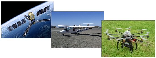
2.2. Remote Sensing Platforms

Three different remote sensing platforms were employed to map the NDVI vegetation index at the two sites (Table 1).

2.2.1. UAV Images

A flight campaign was made on 18 September 2012 using a UAV platform, based on a modified multi-rotor Mikrokopter OktoXL (HiSystems GmbH, Moomerland, Germany) able to fly by remote control or autonomously with the aid of its Global Position System (GPS) receiver and its waypoint navigation system. The sensor utilized to acquire UAV multispectral images was a Tetracam ADC Lite (Tetracam Inc., Chatsworth, CA, USA), described in detail in Table 1. All images were taken between 12:00 and 13:00 in clear sky condition, and a white reference image to compute reflectance was taken by framing a Teflon calibration panel just before the flight. The flight altitude has been fixed at 150 m (AGL), with a UAV flight speed of 4 m/s. Those settings allowed a 72% image forward overlap, while a waypoints route planned ad hoc ensured a 40% image side overlap, high enough to guarantee an optimal photogrammetric processing.
Table 1. Remote sensing platforms.
UAVAIRCRAFTSATELLITE
PlatformMikrokopter OktoXLSky Arrow 650 TC/P68RapidEye
CameraTetracam ADC Lite Remotesensing 07 02971 i001ASPIS Remotesensing 07 02971 i002REIS Remotesensing 07 02971 i003
Number of channels3125
Spectral wavebands520–600 nm
630–690 nm
760–900 nm
415–425 nm
526–536 nm
545–555 nm
565–575 nm
695–705 nm
710–720 nm
745–755 nm
490–510 nm
670–690 nm
770–790 nm
790–810 nm
890–910 nm
440–510 nm
520–590 nm
630–685 nm
690–730 nm
760–850 nm
Dimension114 × 77 × 22 mm270 × 250 × 200 mm656 × 361 × 824 mm
Weight0.2 kg10 kg62 kg
Resolution2048 × 1536 pixel2048 × 2048 pixel12000 pixel linear CCD per band
Pixel size3.2 μm7.4 μm6.5 µm
Focal length8.5 mm12 mm633 mm
FOV42.5° × 32.5°12.5° × 12.5°15.7° × 10.5°
Output data10 bit RAW8 bit RAW16 bit NITF
Image size6 MB4 MB462 MB/25 km along track for 5 bands.
Flight quote AGL150 m2300 m630 km
Flight speed4 m/s90 knot-
Ground resolution0.05 m/pixel0.5 m/pixel5 m/pixel
Ground image dimension116.5 × 87.5 m1024 × 1024 m77 × 45 km
Total frames10021
PixelWrench2 software (Tetracam Inc., Chatsworth, CA, USA) was used to manage and process ADC images, providing a batch file conversion from RAW to TIF. Ortho-rectification of the images was performed by means of a 5 m resolution digital elevation model (DEM). Afterwards, the captured images were assembled into a mosaic by Autopano Pro 3.6 Software (Kolor SARL, Challes-les-Eaux, France). Coordinates of the 50 PVC white panels (0.25 × 0.25 m) randomly located inside each vineyard were measured with a high-resolution (0.02 m) differential GPS Leica GS09 GNSS (Leica Geosystems A.G., Corporate Legal Services, Heerbrugg, Switzerland) to georeference the images. The QGIS software (Quantum GIS Development Team 2014, Quantum GIS Geographic Information System, Open Source Geospatial Foundation Project, http://qgis.osgeo.org) was used to carry out this task, utilizing ground referenced panels and a set of ortho-photos with a ground resolution of 0.5 m. A FieldSpec Pro spectroradiometer (ASD Inc., Boulder, CO, USA) was utilized to perform a radiometric calibration in field as described by Primicerio et al. [6], so each pixel DN (digital number) was converted first into spectral radiance and then into reflectance as described in Goward et al. [11].

2.2.2. Aircraft Images

The aerial data of the two vineyards were acquired on the same day as UAV, in a single swipe with a Sky Arrow ERA platform [12] at a flight altitude of 2300 m above ground level, corresponding to a 0.5 m spatial resolution. The aircraft was equipped with the ASPIS (Advanced SPectroscopic Imaging System) remote sensing system [13] (Table 1), coupled with a Systron Donner C MIGITS III INS/GPS unit (Systron Donner Inertial, Concord, MA, USA) and a Riegl LD90 series laser altimeter (RIEGL Laser Measurement Systems GmbH, Horn, Austria). Spectral bands of red and near infrared were processed in order to calculate NDVI vegetation index. Radiometric correction to the sensor was applied by means of the proprietary software of Terrasystem srl. An atmospheric correction was carried out using the ENVI FLAASH module (Fast Line-of-sight Atmospheric Analysis of Spectral Hypercubes, ITT Visual Information Solutions, USA), an algorithm developed by Spectral Sciences, Inc. (Burlington, MA, USA). Geometric correction, which is necessary to eliminate the internal optical distortions of the sensor and those caused by the altitude, was performed using the software PCI Geomatica (PCI Geomatics Corporate, ON, Canada), through a methodology that envisage the acquisition of ground control points on georeferenced high-resolution images. An aerial model was used as orthorectification algorithm for the aerial data. The aerial orthoimage (a mosaic of two frames) has been returned at 0.50 m ground resolution, and georeferenced in the WGS 84-UTM 32 North reference system.

2.2.3. Satellite Images

A multispectral image acquired on 15 September 2012 (at 11.03 am) was provided by BlackBridge from the RapidEye archive. RapidEye is a constellation of five satellites that acquire multispectral data at a spatial resolution of 6.5 m, resampled to 5 m pixel size, in the range of the visible and near infrared. Images are provided in NITF 16-bit format, while temporal resolution is five to six days for nadir data and one day for the off-nadir. Features of the RapidEye’s spectral bands and technical specification are presented in Table 1. RapidEye Level 2 product embeds radiometric correction natively. As for aerial data, the atmospheric correction was carried out using the ENVI FLAASH module, and the geometric correction with PCI Geomatica software. We used the rational function orthorectification algorithm, while the orthoimage (single frame) has been returned at 5 m ground resolution and then georeferenced in the WGS 84-UTM 32 North reference system.

2.3. Statistical Framework
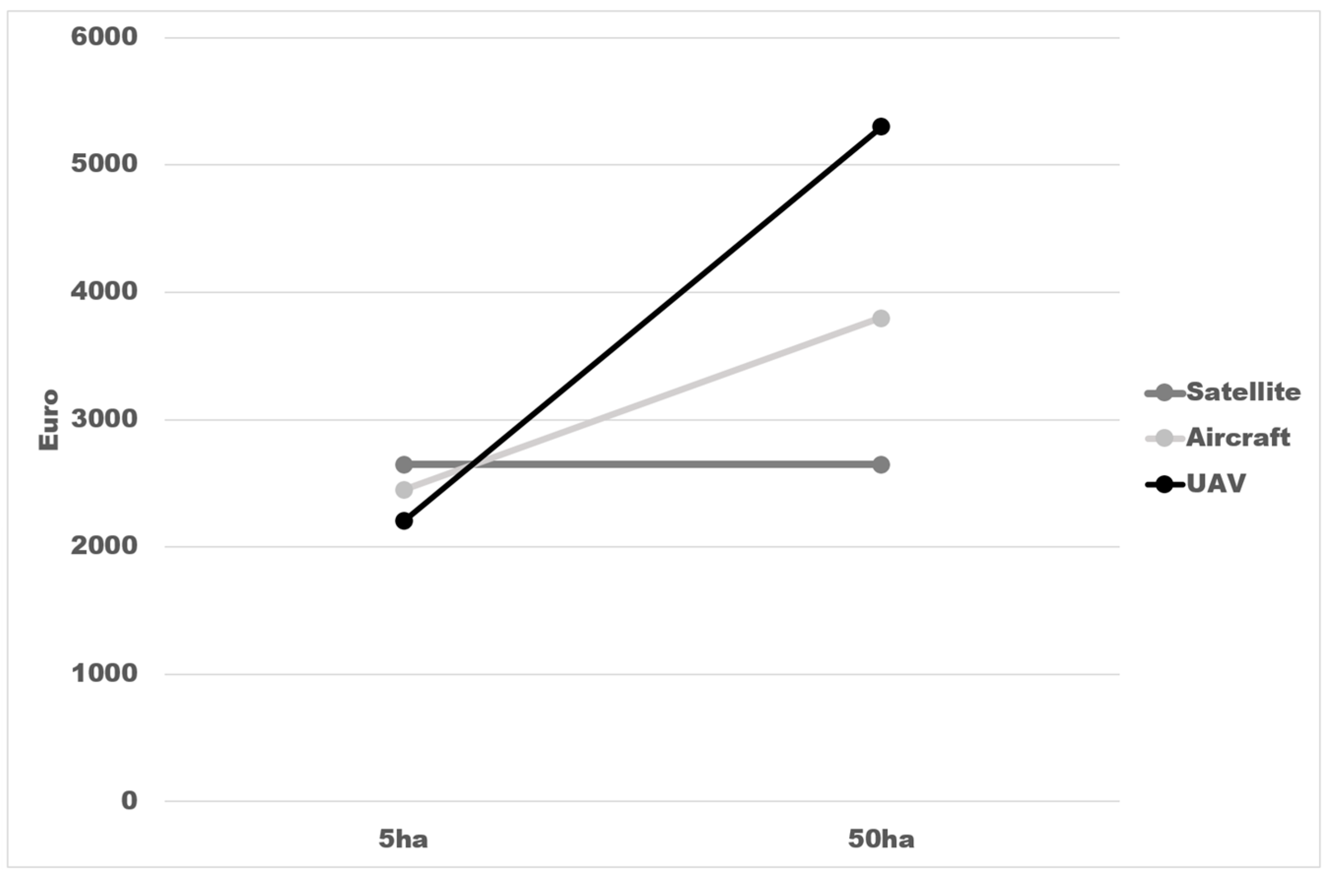
Multispectral images acquired by UAV, aircraft and satellite platforms, were elaborated to calculate NDVI (Normalized Difference Vegetation Index) [14], which is a structural vegetation index utilized for the production of vigor maps according to the methodology extensively described by Matese et al. [8]. A set of statistical tools were applied to analyze the images with different purposes:
Basic statistics and histograms for native resolution images were performed using Matlab software.
Aircraft and UAV images have been resampled to match satellite resolution of 5 m by means of a block-averaging function.
Quadrant decomposition was applied, allowing the decomposition of an image in sub-bocks based on their internal homogeneity: the bigger the sub-blocks, the higher the inherent homogeneity of the image. This method, similarly to a spectrum for a signal, enables the identification of the information that is contained within spatial scales.
The heterogeneity of a map cannot be simply described in terms of descriptive but should account for the spatial structure, or patchiness, of the described variable statistics [15]. CV (coefficient of variation) is a measure of relative variance and was calculated as the ratio of standard deviation to mean value expressed as percentage. For each field, NDVI values were also used to compute geo-statistical information, such as the variogram and the trend (gradient), that were used to assess the within field variability. Native resolution image data were processed using Matlab code in order to calculate the variograms for both the vineyards. Experimental (Semi-) Variogram function [16] calculates the experimental variogram and Variogramfit function [17] performs a least squares fit of various theoretical variograms to an experimental, isotropic variogram. Nugget (N) is the height of the jump of the variogram at the discontinuity at the origin, Sill (S) represent the limit of the variogram tending to infinity lag distances and Range (R) is the distance in which the difference of the variogram from the sill becomes negligible. The variogram was computed using the maximum distance, dmax = 125 m. Trend was calculated using gradient (F) Matlab function, where F is the image matrix and returns the x and y components of the two-dimensional numerical gradient.
The degree of similarity between images can be described by means of similarity indexes able to capture the degree of correlation between spatial structures. In particular two similarity indices, Lee and Pearson, were applied in this work using the map comparison statistic software developed by the Research Institute for Knowledge Systems [18]. Lee’s index [19] offers an approach to calculate bivariate spatial association reconciliating Pearson’s r statistic as a spatial measure of bivariate association and Moran’s I [20] as a univariate measure of spatial association. Basically, the correlation found between the mean fields is corrected for the degree to which X and Y are spatially autocorrelated. Lee index measures the extent to which both map 1 and map 2 are spatially autocorrelated and their neighborhood mean fields are correlated as well. The Pearson correlation (R) was calculated on the basis of a cell-by cell evaluation.

2.4. Cost Analysis

The direct comparison of specific costs for the three platform is nonetheless not feasible due to the different aggregation of their cost estimates [21], as the satellite images are a commercial product where all the operational and development costs are included in the price per image figure and the aircraft campaign utilizes an external vector for aircraft missions. In this study we chose a top-down approach to account for all the expenses associated to data acquisition and processing, grouped into three broad categories:
  • Acquisition costs (C) cover all the expenses to get the raw images. For the satellite this is the purchase price of the commercial image, for the aircraft it includes the cost of the flying vector and the expenses for the deployment of the sensor platform and payload, while for the UAV it includes also all the costs for organizing and conducting the acquisition campaign.
  • Georeferencing and orthorectification (P1) includes the man-hour costs to obtain a georeferred and orthorectified image. The price for a single man-hour was considered at 50 Euros.
  • Image processing (P2) covers all the correction and elaboration, priced in man-hour, needed to get the final results. The process is similar for each platform, the only difference is the different resolution (and hence computing time) of the three starting images, and the fact that satellite and usually aircraft images do not require soil filtering as their resolution do not permit distinguishing between vines and inter-row. Also for that phase 50 Euros per single man-hour was considered.

3. Results and Discussion

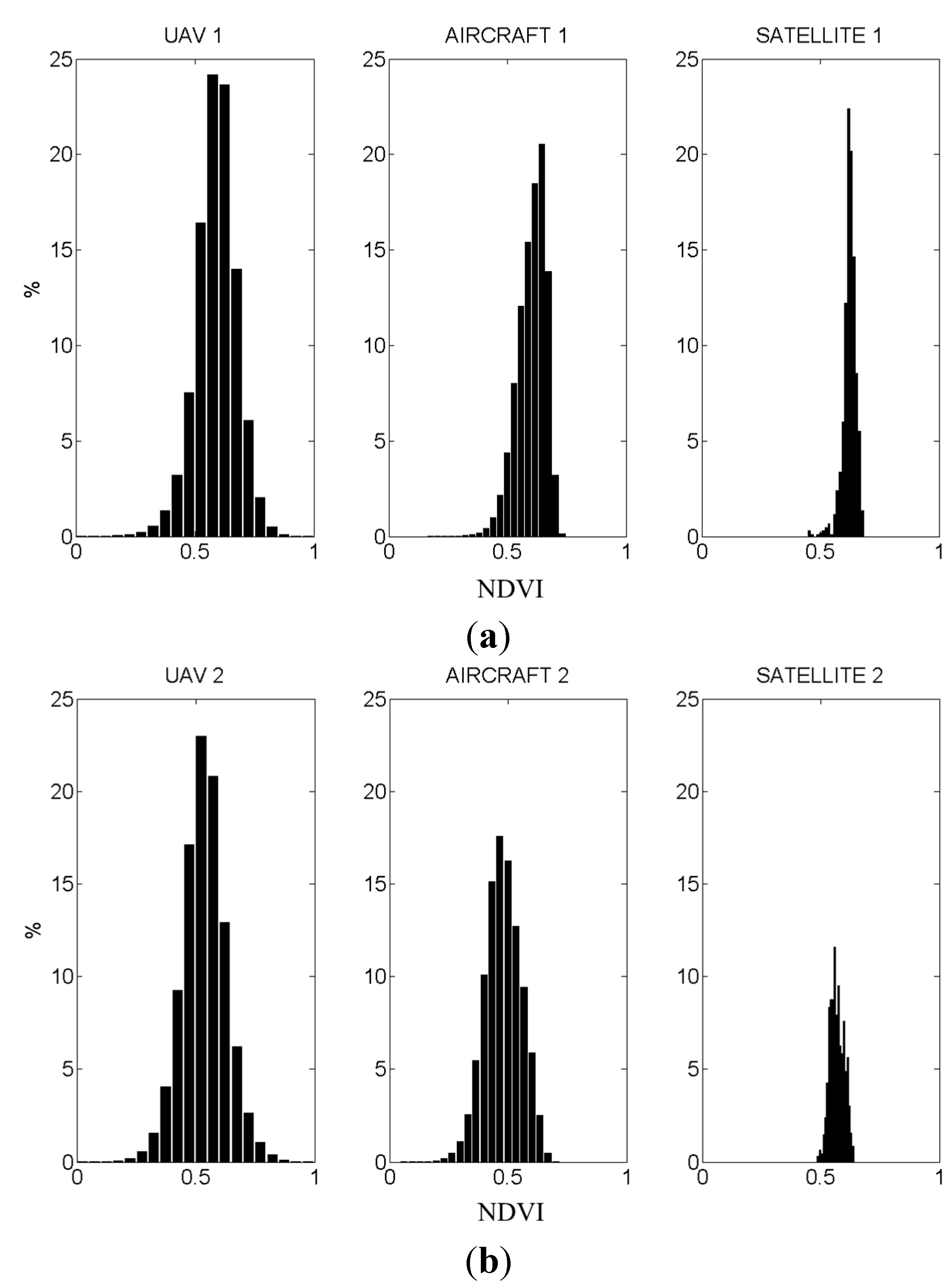
3.1. Histograms and Basic Statistics

The basic statistics performed on the images at native resolution highlighted differences between the three platforms in their range of values. For both V1 and V2 the histogram of UAV values is broader and shows NDVI values between 0.2 and 0.9; values range for aircraft images is between 0.3 and 0.7 while satellite images show a narrower NDVI interval between 0.5 and 0.65 (Figure 1a,b).
This different behavior between the three platforms is also confirmed by the descriptive statistics (Table 2), where UAV images show a higher standard deviation compared to aircraft and satellite images.
Table 2. Basic statistics at native resolution.
PlatformN. ValuesAverageStandard DeviationSkewnessCV (%)Trend (NDVI)
V1–UAV4,956,7890.5890.08−0.3814.610.00005
V1–AIRCRAFT103,1990.6010.06−0.779.980.00054
V1–SATELLITE10120.6240.02−0.283.680.0014
V2–UAV8,233,7910.5360.09−0.1117.160.00037
V2–AIRCRAFT96,5880.4770.07−0.7715.930.00094
V2-SATELLITE9590.5670.030.095.290.0044
Within each platform, the two vineyards did not show substantial differences in the range of values with V1 showing a higher average NDVI and a lower standard deviation, compared to V2 that also has a more Gaussian distribution (Figure 1).
CV was greater in V2 than V1 and more variation going from low (satellite) to high resolution (UAV) was detected. Trend was greater in V2 than V1 showing a regular horizontal drift.
Figure 1. (a) V1 NDVI histogram as percentage of total values; and (b) V2 NDVI histogram.
Remotesensing 07 02971 g001
The larger range of values (Figure 1) and the higher coefficient of variability (CV) detected by the UAV platform is explained by its higher resolution, which in a highly heterogeneous crop, such as vineyards, enables the identification of the alternation of canopies (higher NDVI values) and inter-rows (lower NDVI values related to grass cover or bare soil). On the contrary, the typical vineyard discontinuity was not detected by the satellite resolution that averages canopy and inter-row reflectance values, therefore providing a narrower distribution. Aircraft data fall in between UAV and satellite in terms of NDVI histograms (Figure 1) and variability (Table 1), confirming that spatial resolution is the key parameter controlling the amount of spatial information that is effectively sampled by each instrument.

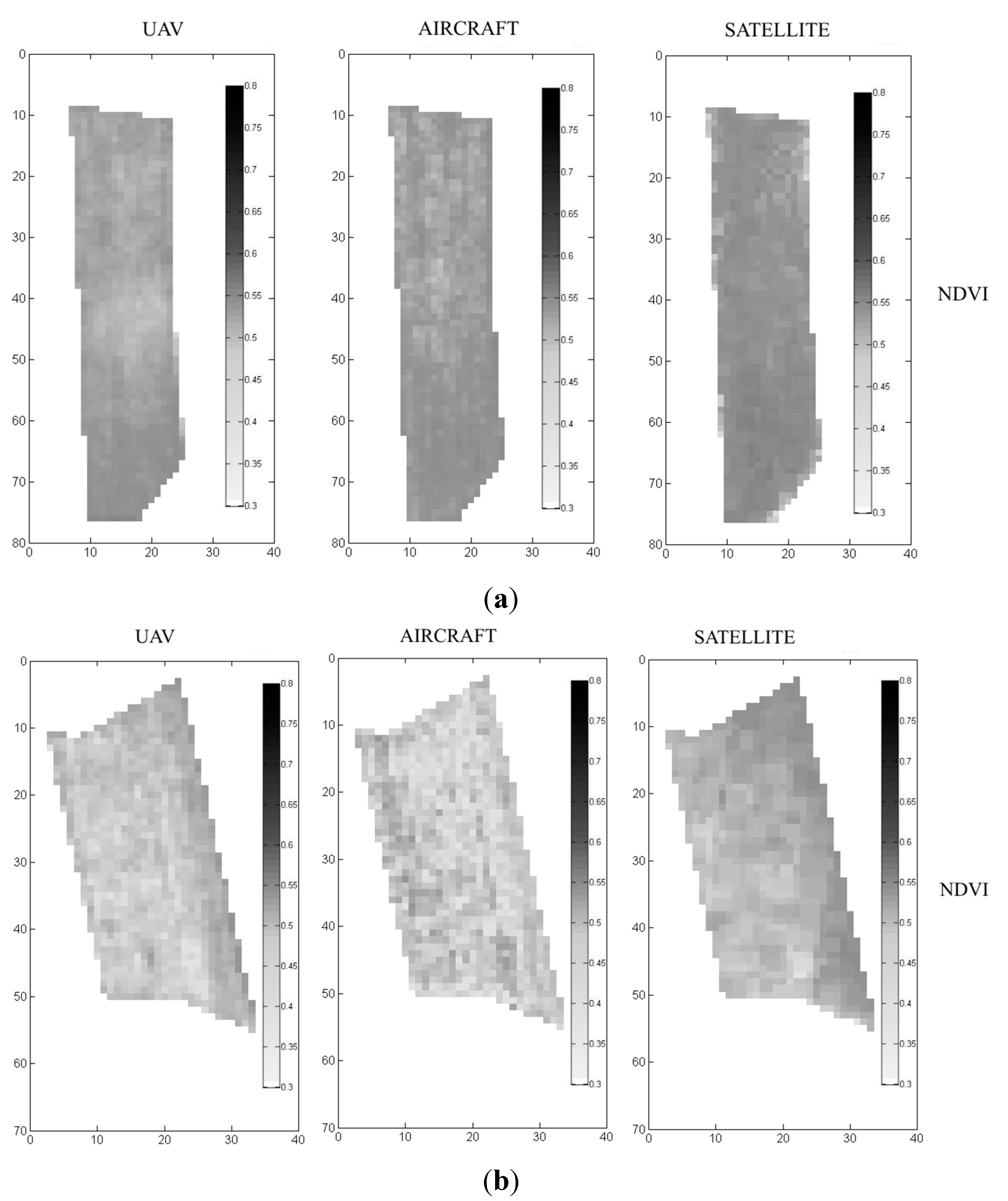
3.2. Coarse Resolution Inter-Comparison

The comparison of images from the three platforms after the re-scaling at the satellite resolution (5 m) highlights similar behaviors of vegetation patterns and their spatial structure showing also some differences among platforms (Figure 2a,b).
From a visual inspection of the V1 images, a low vigor zone can be observed in the UAV image in the central zone of V1 that is progressively less pronounced in the aircraft and then in satellite image (Figure 2a). Similarly, vineyard 2 shows a gradient in the West-East direction that is more evident in satellite images while it is smoother in the UAV images and the aircraft pattern shows a more abrupt distribution in two distinct macro zones along the same direction (Figure 2b).
Figure 2. (a) V1 images rescaled at 5-m resolution for the three platforms; and (b) V2 images rescaled at 5-m resolution for the three platforms.
Remotesensing 07 02971 g002
The similarity analysis enabled a further insight of these analogies and discrepancies: higher correlations were observed between UAV and aircraft images for both vineyards (R = 0.635 for V1 and R = 0.881 for V2) (Table 3), while the correlation between UAV and satellite was high for V2 (R = 0.779) and low for V1 (R = 0.286). Similarly, aircraft vs. satellite correlation was high in V2 (0.78) and low in V1 (0.42). Lee’s similarity index was high for V2 between all platforms and only between UAV and aircraft for V1. Overall, all the cross-platform combinations of Pearson correlation and Lee index had consistently larger values in V2 than V1, suggesting that the presence of gradients and spatial patterns, like those observed in V2 (Figure 2), tends to increase spatial correlation parameters. On the other hand, more homogeneous patterns like in V1 are intrinsically less correlated. In terms of statistical comparison, the lower resolutions seems more informative in presence of vineyards showing variability according to a spatial gradient (trend), with respect to more homogeneous vineyards or vineyards showing a more irregular vegetation distribution (lower trend).
Table 3. Similarity analysis indices.
V1V2
Pearson (R)Lee (L)Pearson (R)Lee (L)
SATELLITE vs. UAV0.2860.2460.7990.701
SATELLITE vs. AIRCRAFT0.4260.3460.7760.689
AIRCRAFT vs. UAV0.6350.5470.8810.747

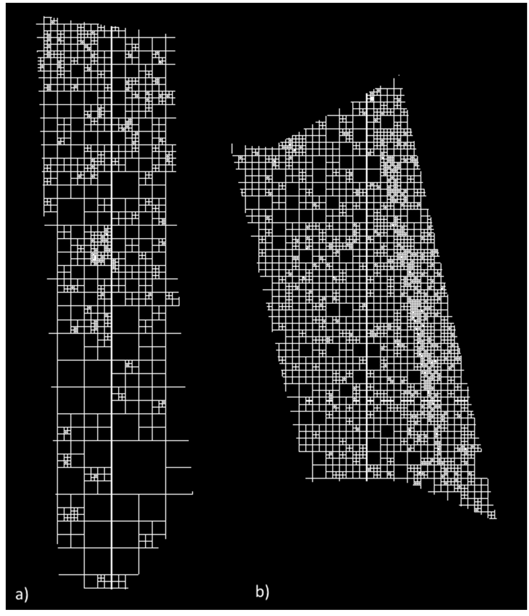
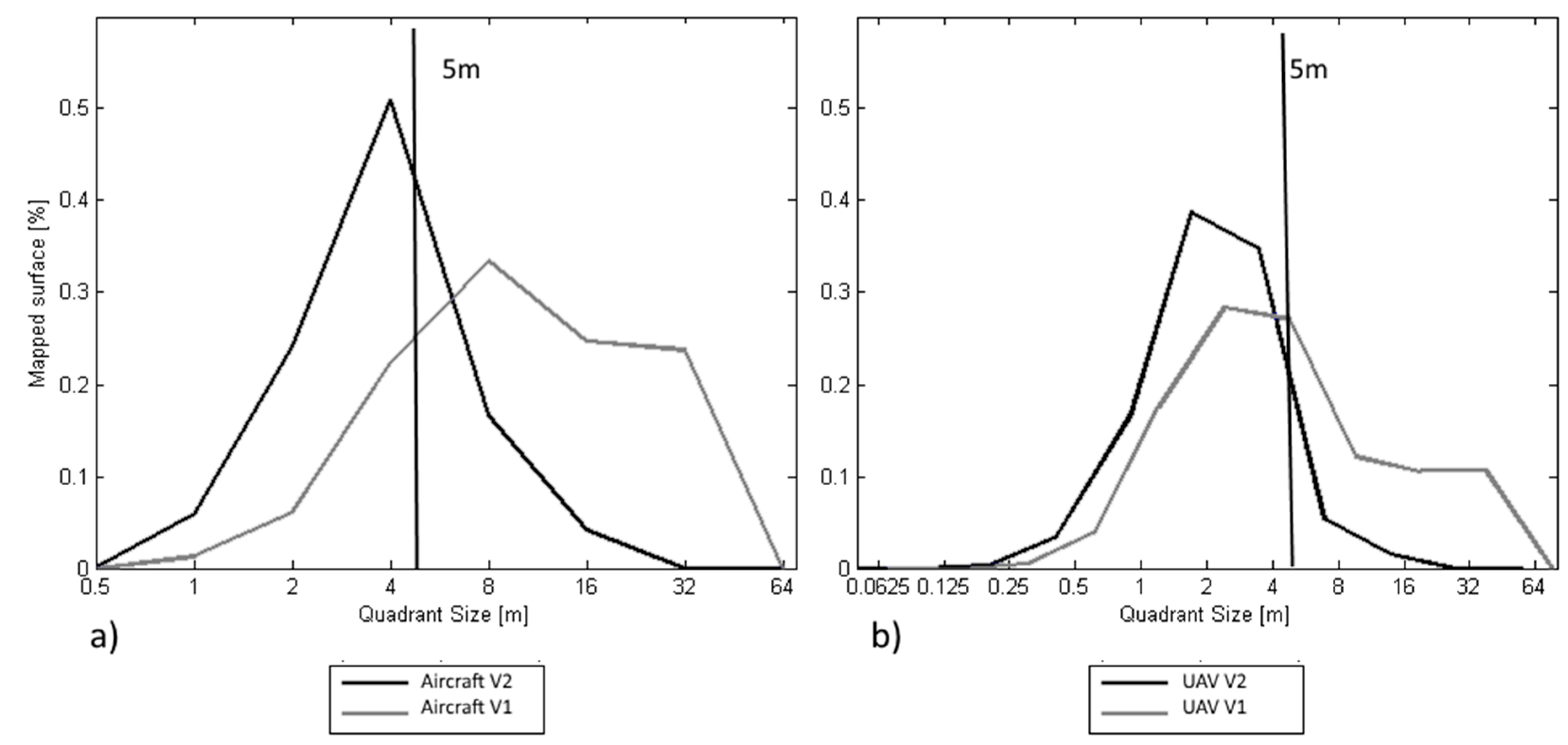
3.3. Image Decomposition

The analysis of image structure performed on aircraft images with the quadrant decomposition method highlights a substantial difference in the distribution of dimensional classes between the two vineyards. V2 showed a higher degree of fragmentation, in particular in the east part, while V1 is represented by larger blocks and has therefore more homogeneous zones (Figure 3a,b).
Figure 3. (a) V1 quadrant decomposition results and (b) V2 quadrant decomposition results.
Remotesensing 07 02971 g003
The distribution of dimensional classes differs between the two vineyards and is consistent between the two platforms (UAV and aircraft).
The decomposition of V1 showed a higher presence of larger classes, especially in the aircraft image decomposition, while V2 was more heterogeneous and well represented by smaller classes. The smaller classes represented are those of the native resolution of each acquisition platform (0.05 and 0.5 m for UAV and Aircraft, respectively).
The analysis of the curves in Figure 4 enabled the quantification of the level of information that is not resolved moving from UAV and Aircraft to satellite resolution. Considering that satellite resolution is 5 m (represented by the dashed line in Figure 5), this spatial decomposition highlights how a relatively large fraction of information is represented by classes actually smaller than the satellite resolution. But it is worth noting that such fraction is higher in V2 with respect to V1, this means that satellite resolution is able to provide an appropriate representation of vineyards in those cases where the spatial structure of vegetation is more homogeneous.
Figure 4. (a) Distribution of dimensional classes for Aircraft resolution and (b) distribution of dimensional classes for UAV resolution.
Remotesensing 07 02971 g004

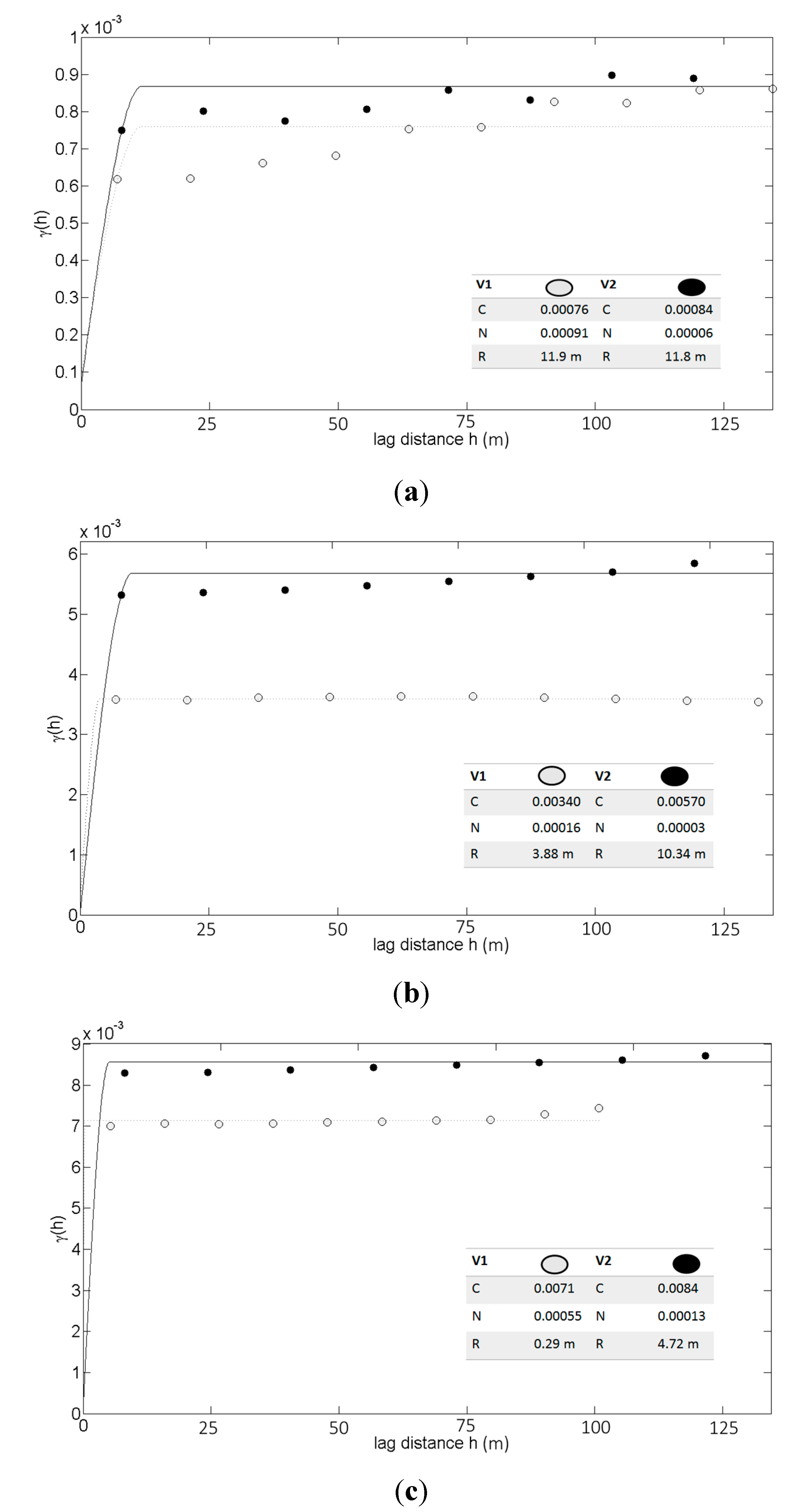
3.4. Variogram Analysis

The trend of variogram (Figure 5) variations with the spatial resolution describes the effect of spatial heterogeneity, providing an assessment of NDVI spatial structures within the image domain [22]. In general, all the variograms computed on all the images reached a sill well before dmax (maximum distance). The sill is an indicator of the spatial variability of the data.
All experimental variograms computed on the images are linear at the origin, without any nugget effect, then increase promptly and reach almost the whole image variance at a very short range in V1 for UAV and AIRCRAFT (Raircraft = 3.88 m; Ruav = 0.29 m) with respect to V2 (Raircraft = 10.34 m; Ruav = 4.72 m), confirming that V1 is poorly structured with respect to V2 (Figure 5a–c). The degree of image spatial variability was attributable to the sill and for all the platforms it was higher in V2 than in V1 and was higher for UAV than aircraft and satellite.
Figure 5. NDVI variograms of three platforms at native resolutions. The lines represent the fitted variograms models. The parameter of the variogram model are reported in the legend: C = sill, N = nugget, and R = range. (a) Satellite, (b) Aircraft, and (c) UAV
Remotesensing 07 02971 g005
The analysis of images fragmentation, performed with variograms and quadrant decomposition, provided a further insight highlighting the importance of the typology of vegetation structure fragmentation: V1 was characterized by larger clusters of vegetation while V2 is characterized by higher heterogeneity and smaller vegetation sub-classes. With this approach, V1 distribution of pixels clustering, results are consistent between UAV and aircraft acquisition, confirming a distribution toward larger classes. For this vineyard (V1), all remote sensing platforms appear to be highly informative independently from their native resolution; in fact most of the variability falls in the bigger classes (>2 m), thus closer to the satellite native resolution. On the contrary, V2 vineyard was characterized by a higher variability and the classes of information that cluster together are placed at substantially smaller resolution and, in this case, the satellite platform succeeds only in part to represent the variability of the vineyard that is for over 50% described by classes smaller than the satellite resolution.
The images comparative analysis acquired by the three different platforms involved the use of different methodologies in order to understand if when scaled to the spatial resolution of the satellite, these were comparable. The results show that the loss of information at lower resolution (satellite) relative to the aircraft and UAV are variable between vineyards, and cannot be simply described by pixel-based statistical indexes, such as Pearson correlation. In fact, V2 showed either a higher fragmentation into small spatial scales that are not resolved by the satellite platform (Figure 4b and 5b), and higher values of Pearson correlation and Lee indexes at the 5 m satellite resolution, with respect V1 (Table 1). These results indicate that high Pearson correlation and Lee values at coarse resolution do not provide any insight of the actual amount of spatial variability that is contained in smaller classes, which can only be quantified with structural and variogram analysis.
Other authors, as reported by Garrigues et al. [22], have studied many methods to quantify spatial heterogeneity from empirical (i.e., local variance), probabilistic (i.e., Variogram and fractal) to mathematical (i.e., Fourier or wavelet transform, but mainly applied to low-resolution images and comparing different satellite sensors). D’Oleire-Oltmanns et al. [23] compared UAV and satellite images for soil erosion assessment, proving an identification of gullies on different scales. Hall et al. [24] presented a review of remote sensing platforms, satellite and aircraft, demonstrating the high potential application of such technologies in precision viticulture.

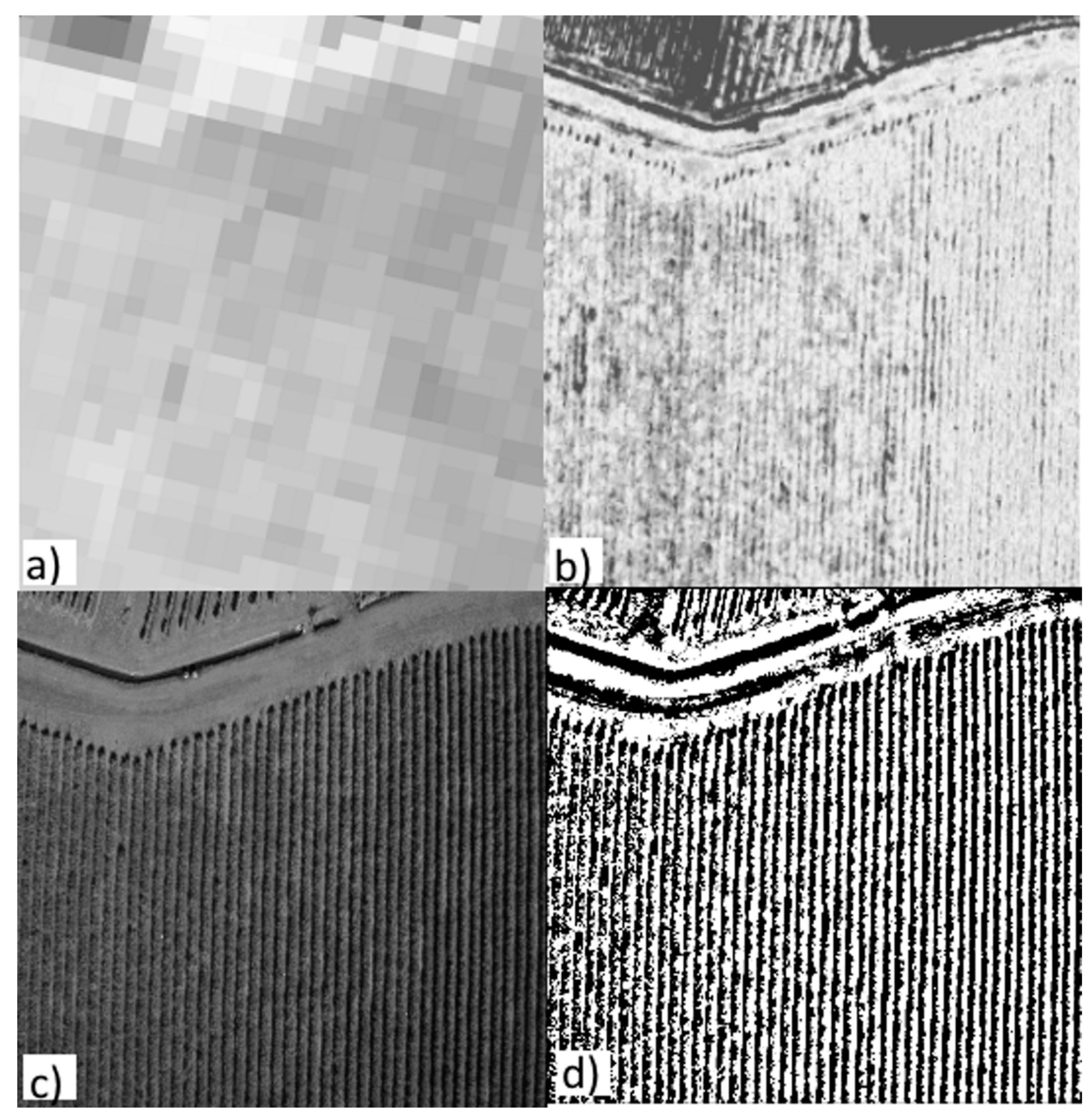
3.5. Inter-Row Separation

Remote sensing representation of vineyards presents specific peculiarities, because of the alternation of vertical vine canopies with a horizontal surface that can be bare soil or covered by grass. This characteristic implies that the remotely sensed images contain information other than the vine canopy, i.e., the inter-row soil and the shading produced by canopies. In this sense, while satellite resolution necessarily implicates the averaging of row and inter-row information, smaller resolution of the same order of magnitude of canopy projection, enables performing a filtering of the image with the purpose of excluding the information coming from the inter-row. The possibility of removing the spectral response of the inter-row is of particular interest in the case of grass-covered inter-rows that can result in a biased representation of vine canopy status. This procedure can be easily performed starting from UAV images by mean of establishing a region of interest (ROI) in the center of each vine row with a canopy buffer width [25]. A comparison of images from the three resolutions with an inter-row filtering applied to UAV images is provided in Figure 6.
Figure 6. (a) Vineyard portion of Satellite image; (b) Vineyard portion of Aircraft image; (c) Vineyard portion of UAV image; and (d) Vineyard portion of UAV image with inter-row filtering.
Remotesensing 07 02971 g006

3.6. Acquisition and Processing Cost Analysis

The three different platform analyzed in this study provide data products that illustrate the capability of remote sensing technologies to monitor and map vineyards with different levels of accuracy, emphasizing the impact of spatial resolution on vineyard variability assessment and analysis.
The cost analysis was applied at two different spatial scales related to our study: 5 ha, which was the area actually mapped by UAV in this study, and 50 ha, which was the area actually mapped by the aircraft survey. Table 4 summarizes the operational costs associated with this case study. The number of images required to map a certain area (N) scales exponentially from satellite to aircraft and UAV, also resulting an increasing cost for the image processing chain (P1 and P2). The acquisition cost was fixed for satellite at both scales, since the same image can cover both areas, while it increases from 5 to 50 ha by a factor of 1.36 and 2.66 for aircraft and UAV, respectively.
The cost/benefit analysis was calculated on the basis of a service that is offered by a third party, thus not including the investment cost of purchasing an aerial platform or a UAV, instrumentation, maintenance, etc. Overall, on small fields (5 ha) the use of UAV appears to be the most cost effective solution due to the low cost for the data acquisition (Figure 7). On the contrary, when the plots reach a larger dimension (50 ha analyzed here), the UAV solution appears to be the least economic. The satellite solution does not imply any significant difference, while the aircraft solution is placed in the middle, showing only a marginal additional cost in the data acquisition related to the slightly higher flight time, and some higher image processing costs, since the typical aircraft acquired image was in the order of 8–10 ha, requiring the processing of multiple images in the 50 ha case, and only one image in the 5 ha case. The break-even point that can be derived from Figure 7, i.e., the point at which two or more lines intercept, is placed slightly above 5 ha for all three platforms, meaning that at such scale size, the three technologies have approximately the same acquisition and processing cost.
Table 4. Category costs (Euro) for satellite, aircraft and UAV mapping. N is the number of images that compose the mosaick, C the acquisition costs, P1 the georeferencing and orthorectifing costs and P2 the image processing costs.
5 ha50 ha
NCP1P2NCP1P2
Satellite12500501001250050100
Aircraft12200100150103000500300
UAV1001500500200100040001000300
Figure 7. Plot of category costs (Euro) for satellite, aircraft and UAV platform, considering a 5 ha and 50 ha mapping area.
Remotesensing 07 02971 g007
The presented techniques are promising tools for farmers to monitor their crops, but each of them, if analyzed individually, can often be incomplete. In fact, if on one hand the applications of UAV and aircraft may be optimal for a fine characterization of the fields in terms of resolution and to identify the intra-vineyard variability, on the other hand satellite remote sensing is capable of mapping field variability with a higher temporal continuity that is consistent across seasons and multiple years, allowing monitoring of different vegetation stages during the growing season and to derive an historic analysis on past seasons.
However, a parameter that can better target farmers to choose one or the other platform, or towards a multiplatform approach, is represented by the real structure of the vineyard that can be assessed only by UAV or aircraft application. It is hard, with satellite-only images, to assess factors, such as the actual degree of heterogeneity of the field, the status of the inter-row area, and therefore to assess the uncertainties associated with the satellite representation, lacking a fine resolution truth. In the presence of pronounced intra-vineyard variability associated with a lack of well-defined structure and gradients, drones and aircraft can provide valuable information to tailor the use of pesticides, herbicides, fertilizer and other applications based on how much is needed at a specific point in a field, saving the grower money from unnecessarily overusing resources, while at the same time reducing the amount of runoff that could flow into nearby rivers and streams.
Table 5 is an attempt to integrate all factors considered in this study, summarizing the strengths and weaknesses of the three platforms used as experienced in the actual acquisition campaigns. The mission attributes deal with the planning and execution of the surveys, the ability to reach the site (Range), to deal with weather condition and scheduled practices of the farm (cloud cover and flexibility), the need of multiple flights to obtain the whole scene (Endurance), and the overall reliability of the platform installment. With respect to aircraft and satellite, UAV can operate closer to the target with more flexibility on scheduling, and its acquisition are non-dependent on cloud cover conditions, but has a much shorter range and endurance and an overall lower reliability, being still in the prototyping phase. Satellite images on the contrary cover much larger areas, but are subject to fixed scheduling and strongly depend on cloud cover. The aircraft platform sits in between these two with more flexibility than satellite and better endurance than UAV.
Table 5. Comparative platform characteristics for different remote sensing platforms. (++ optimal, + good, o average, - poor).
UAVAircraftSatellite
MissionRange-+++
Flexibility+++-
Endurance-++++
Cloud cover dependency+++-
Reliabilityo+++
ProcessingPayloado+++
Resolution+++o
Precision+++o
Mosaicking and geocoding effort-o++
Processing timeo++
The image processing attributes deal with the computational chain deployed from the raw images to the final products. It includes the precision and resolution attainable on the maps and the effort and computing time to mosaic, orthorectify and produce the outputs. The strengths of UAV acquisition are of course in the higher resolution and precision, but at the cost of a greater effort for mosaicking and geocoding. Given the low number of images in the aircraft survey, an almost automatic processing code was implemented, reducing time and costs of elaboration. Satellite images on the contrary require no mosaicking and geocoding, at the price of a much lower resolution. The lower payload of the UAV platform while requiring dedicated and miniaturized sensors, was not a limiting factor in our acquisition campaigns

3.7. Operational Discussions

In the context of PV, vegetation mapping serve as a base to perform variable rate applications (VRAs). In this sense, from an operational perspective, the different platforms might be used with different purposes and provide input for different variable rate applications. One of the most interesting VRA applications is the Variable Rate Spraying that consist in dosing the quantity of pesticides in function of the canopy volume, a technique that proved to enable an overall saving of up to 58% of application volume [26] with consequent reduction of pollution and of operation costs. In this specific case, high-resolution images are likely to represent the optimal solution for an efficient dosing of treatment, while low-resolution satellite images risk underestimating the canopy volume and therefore drive the application of insufficient treatment coverage.
On the contrary, in the case of other VRAs, such as selective harvesting, a technique that enables the machine selection and harvesting of grapes of different qualitative classes and with different product destinations [27], the use of low-resolution images would provide a sufficiently accurate representation of grape quality macro-classes.
A further aspect to be considered is that the low spatial resolution cannot account for inter-row management practice and, as a final result, it outputs an averaged spectral reflectance of the canopy and inter-row, independently from the agronomic management adopted.

4. Conclusions

The understanding of the intra-vineyard variability is a keystone to implement effective PV practices, especially in Mediterranean environment where the land-use patterns are highly fragmented and vineyards present high heterogeneity because of soil, morphology and microclimate variability. Our study, based on the comparison of different remote sensing platforms, highlighted that different resolutions provide similar results in the case of vineyards characterized by pronounced vegetation gradients and large vegetation clusters. On the contrary, in vineyards characterized by small vegetation gradients and high vegetation patchiness, low resolution images fail in representing intra-vineyard variability and its patterns. Furthermore, considering the peculiarity of vineyards crop structure, our work points out the impossibility of distinguishing canopy and inter-rows in the case of low-resolution images, something that limits the applicability of this platforms in the case of variable rate spraying.
The cost analysis shows that, beyond technical aspects, an economic break-even between UAV and the other platforms exists between 5 and 50 ha of area coverage, and also that aircraft remote sensing remains competitive with satellite above such threshold.

Acknowledgments

This work was supported by a grant from the Italian Ministry of Economy and Finance for the project “Innovazione e Sviluppo del Mezzogiorno-Conoscenze Integrate per Sostenibilità ed Innovazione del Made in Italy Agroalimentare-Legge n. 191/2009” and by the Italian MIUR (Progetto Premiale AQUA to CNR).
We gratefully acknowledge BlackBridge (www.BlackBridge.com) for RapidEye satellite image and Iptsat srl, the Italian local official distributor of RapidEye (www.iptsat.com) for data analysis support. The authors are grateful to Netherlands Environmental Assessment Agency (MNP) as the owner and RIKS BV as the developer of the MCK software.

Author Contributions

Alessandro Matese conceived and designed the experiments, supported the statistical analysis, and wrote the manuscript. Piero Toscano performed the statistical data analysis and wrote the manuscript. Salvatore Filippo Di Gennaro proposed the field trial’s design and supported the statistical analysis. Lorenzo Genesio analyzed the data and wrote the manuscript. Francesco Primo Vaccari supported the field experiment and helped with editorial contributions. Jacopo Primicerio performed the UAV flights and worked on the costs and comparisons between the platforms. Claudio Belli performed the aircraft flights. Alessandro Zaldei supported in development and measurements. Roberto Bianconi analyzed aircraft and satellite images. Beniamino Gioli processed the imagery and helped with editorial contributions.

Conflicts of Interest

The authors declare no conflict of interest.

References

  1. Whelan, B.M.; McBratney, A.B. The “null hypothesis” of precision agriculture management. Precis. Agric. 2000, 2, 265–279. [Google Scholar] [CrossRef]
  2. Bramley, R.G.V.; Hamilton, R.P. Understanding variability in winegrape production systems. 1. Within vineyard variation in yield over several vintages. Aust. J. Grape Wine Res. 2004, 10, 32–45. [Google Scholar] [CrossRef]
  3. Salamí, E.; Barrado, C.; Pastor, E. UAV flight experiments applied to the remote sensing of vegetated areas. Remote Sens. 2014, 6, 11051–11081. [Google Scholar] [CrossRef] [Green Version]
  4. Kelcey, J.; Lucieer, A. Sensor correction of a 6-band multispectral imaging sensor for UAV. Remote Sens. 2012, 4, 1462–1493. [Google Scholar] [CrossRef]
  5. Zarco-Tejada, P.J.; González-Dugo, V.; Berni, J.A.J. Fluorescence, temperature and narrow-band indices acquired from a UAV platform for water stress detection using a micro-hyperspectral imager and a thermal camera. Remote Sens. Environ. 2012, 117, 322–337. [Google Scholar] [CrossRef]
  6. Primicerio, J.; Di Gennaro, S.F.; Fiorillo, E.; Genesio, L.; Lugato, E.; Matese, A.; Vaccari, F.P. A flexible unmanned aerial vehicle for precision agriculture. Precis. Agric. 2012, 13, 517–523. [Google Scholar] [CrossRef]
  7. Zhang, C.; Kovacs, J.M. The application of small unmanned aerial systems for precision agriculture: A review. Precis. Agric. 2012, 13, 693–712. [Google Scholar] [CrossRef]
  8. Matese, A.; Capraro, F.; Primicerio, J.; Gualato, G.; Di Gennaro, S.F.; Agati, G. Mapping of vine vigor by UAV and anthocyanin content by a non-destructive fluorescence technique. In Proceedings of the 9th European Conference on Precision Agriculture (ECPA), Lleida, Spain, 7–11 July 2013.
  9. Hunt, E.R., Jr.; Hively, W.D.; Fujikawa, S.; Linden, D.; Daughtry, C.S.; McCarty, G. Acquisition of NIR-Green-Blue digital photographs from unmanned aircraft for crop monitoring. Remote Sens. 2010, 2, 290–305. [Google Scholar] [CrossRef]
  10. Berni, J.; Zarco-Tejada, P.; Suarez, L.; Fereres, E. Thermal and narrowband multispectral remote sensing for vegetation monitoring from an unmanned aerial vehicle. IEEE Trans. Geosci. Remote Sens. 2009, 47, 722–738. [Google Scholar] [CrossRef]
  11. Goward, S.N.; Markham, B.; Dye, D.G.; Dulaney, W.; Yang, J. Normalized difference vegetation index measurements from the advanced very high resolution radiometer. Remote Sens. Environ. 1991, 35, 257–277. [Google Scholar] [CrossRef]
  12. Gioli, B.; Miglietta, F.; Vaccari, F.P.; Zaldei, A.; de Martino, B. The sky arrow ERA, an innovative airborne platform to monitor mass, momentum and energy exchange of ecosystems. Ann. Geophys. 2006, 49, 109–116. [Google Scholar]
  13. Papale, D.; Belli, C.; Gioli, B.; Miglietta, F.; Ronchi, C.; Vaccari, F.P.; Valentini, R. ASPIS, A flexible multispectral system for airborne remote sensing environmental applications. Sensors 2008, 8, 3240–3256. [Google Scholar] [CrossRef]
  14. Rouse, J.W., Jr.; Haas, R.H.; Schell, J.A.; Deering, D.W. Monitoring vegetation systems in the Great Plains with ERTS. In Proceedings of the Third ERTS Symposium, NASA SP-351, Washington, DC, USA, 10–14 December 1973.
  15. Pringle, M.J.; McBratney, A.B.; Whelan, B.M.; Taylor, J.A. A preliminary approach to assessing the opportunity for site-specific crop management in a field, using yield monitor data. Agric. Syst. 2003, 76, 273–292. [Google Scholar] [CrossRef]
  16. Matlab Central (Experimental (Semi-) Variogram function by Wolfgang Schwanghart). Available online: http://www.mathworks.com/matlabcentral/fileexchange/20355-experimental-semi-variogram (accessed on 1 September 2014).
  17. Matlab Central (variogramfit function by Wolfgang Schwanghart). Available online: Http://www.mathworks.com/matlabcentral/fileexchange/25948-variogramfit (accessed on 1 September 2014).
  18. Visser, H.; de Nijs, T. The map comparison kit. Environ. Modell. Softw. 2006, 21, 346–358. [Google Scholar] [CrossRef]
  19. Lee, S.I. Developing a bivariate spatial association measure: An integration of Pearson’s r and Moran’s I. J. Geogr. Syst. 2001, 3, 369–385. [Google Scholar] [CrossRef]
  20. Moran, P.A.P. The interpretation of statistical maps. J. R. Statist. Soc. 1948, 37, 243–251. [Google Scholar]
  21. Valerdi, R.; Merrill, J.; Maloney, P. Cost metrics for unmanned aerial vehicles. In Proceedings of the AIAA 16th Lighter-Than-Air Systems Technology Conference and Balloon Systems Conference, Arlington, VA, USA, 26–28 September 2005.
  22. Garrigues, S.; Allard, D.; Baret, F.; Weiss, M. Quantifying spatial heterogeneity at the landscape scale using variogram models. Remote Sens. Environ. 2006, 103, 81–96. [Google Scholar] [CrossRef]
  23. D’Oleire-Oltmanns, S.; Marzolff, I.; Peter, K.D.; Ries, J.B.; Aït Hssaïne, A. Monitoring soil erosion in the Souss Basin, Morocco, with a multiscale object-based remote sensing approach using UAV and satellite data. In Proceedings of the 1st World Sustainability Forum, Sciforum Electronic Conference Series, 1–30 November 2011; Available online: http://www.sciforum.net/conference/wsf/paper/562 (accessed on 9 March 2015).
  24. Hall, A.; Lamb, D.W.; Holzapfel, B.; Louis, J. Optical remote sensing applications in viticulture–A review. Aust. J. Grape Wine Res. 2002, 8, 36–47. [Google Scholar] [CrossRef]
  25. Zarco-Tejada, P.J.; González-Dugo, V.; Williams, L.E.; Suárez, L.; Berni, J.A.J.; Goldhamer, D.; Fereres, E. A PRI-based water stress index combining structural and chlorophyll effects: Assessment using diurnal narrow-band airborne imagery and the CWSI thermal index. Remote Sens. Environ. 2013, 138, 38–50. [Google Scholar] [CrossRef]
  26. Llorens, J.; Gil, E.; Llop, J.; Escolà, A. Variable rate dosing in precision viticulture: Use of electronic devices to improve application efficiency. Crop Prot. 2010, 29, 239–248. [Google Scholar] [CrossRef] [Green Version]
  27. Bramley, R.G.V.; le Moigne, M.; Evain, S.; Ouzman, J.; Florin, L.; Fadaili, E.M. On-the-go sensing of grape berry anthocyanins during commercial harvest: Development and prospects. Aust. J. Grape Wine Res. 2011, 17, 316–326. [Google Scholar] [CrossRef]

