
Improvements of a COMS Land Surface Temperature Retrieval Algorithm Based on the Temperature Lapse Rate and Water Vapor/Aerosol Effect

Abstract
:
1. Introduction
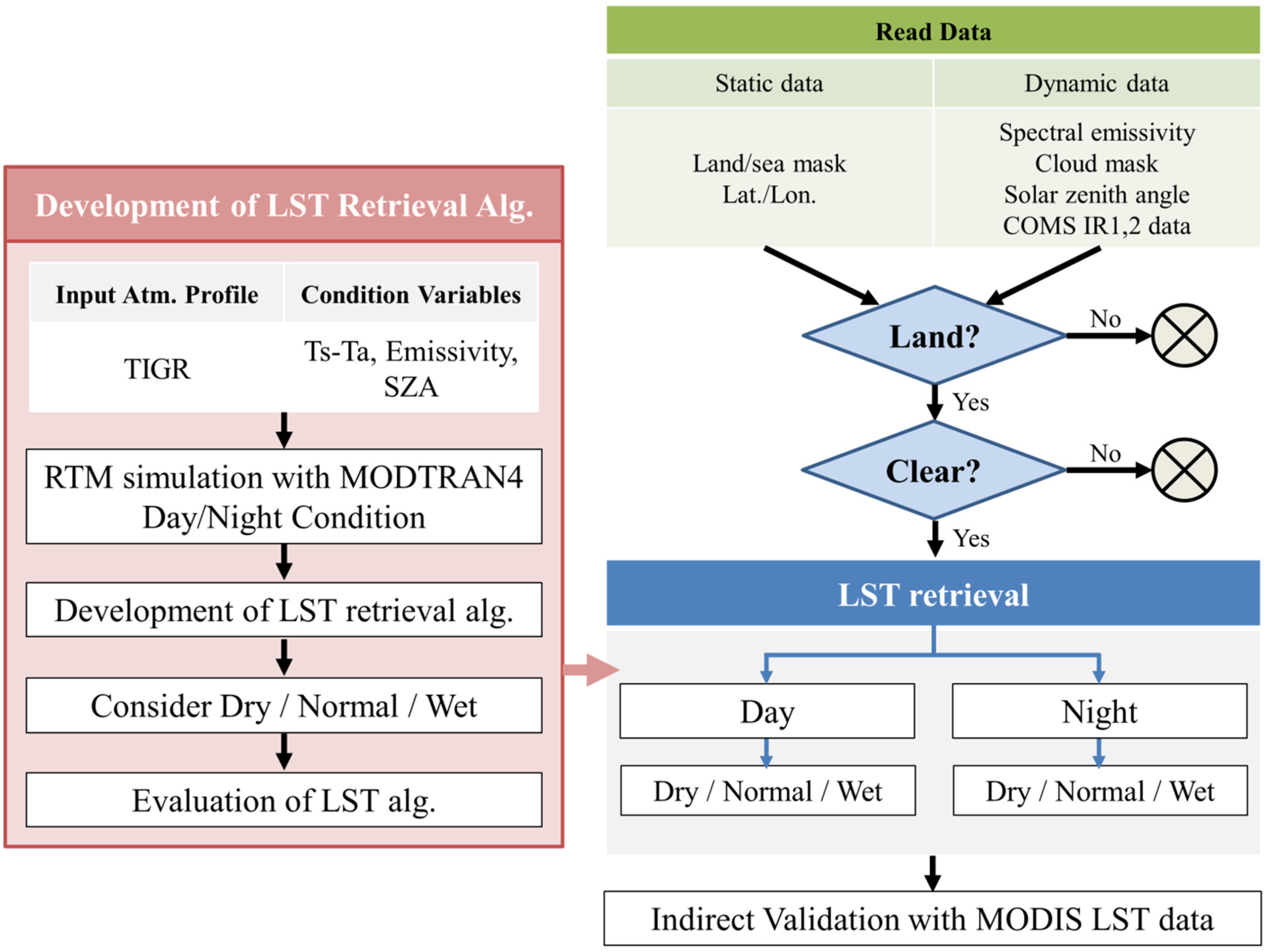
2. Data and Methods
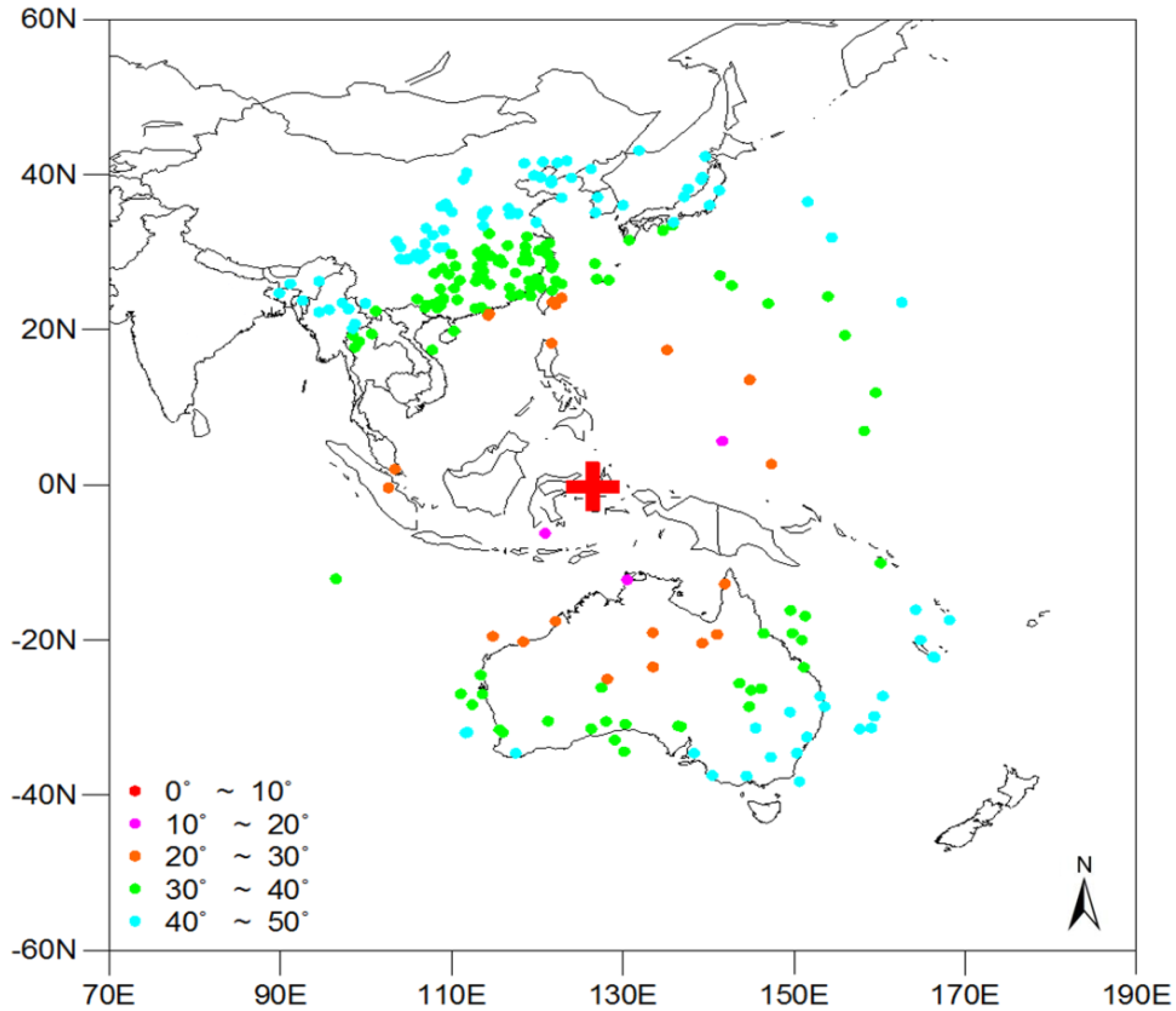
2.1. Data
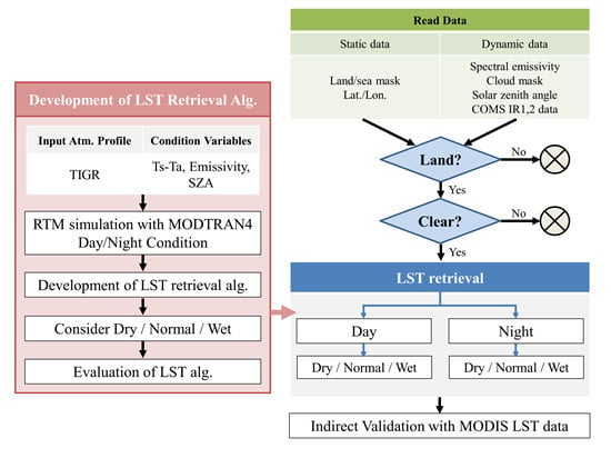
2.2. Methods

| Conditions | BTD Ranges | LST Equation |
|---|---|---|
| Dry | BTD < 0 | (2) for Day, (5) for Night |
| Dry-Normal | −1 ≤ BTD ≤ 1 | Day: weighted sum of (2) and (3) |
| Normal | 0 < BTD < 4 | (3) for Day, (6) for Night |
| Normal-Wet | 3 ≤ BTD ≤ 5 | Day: weighted sum of (3) and (4) |
| Wet | BTD > 4 | (4) for Day, (7) for Night |
3. Results
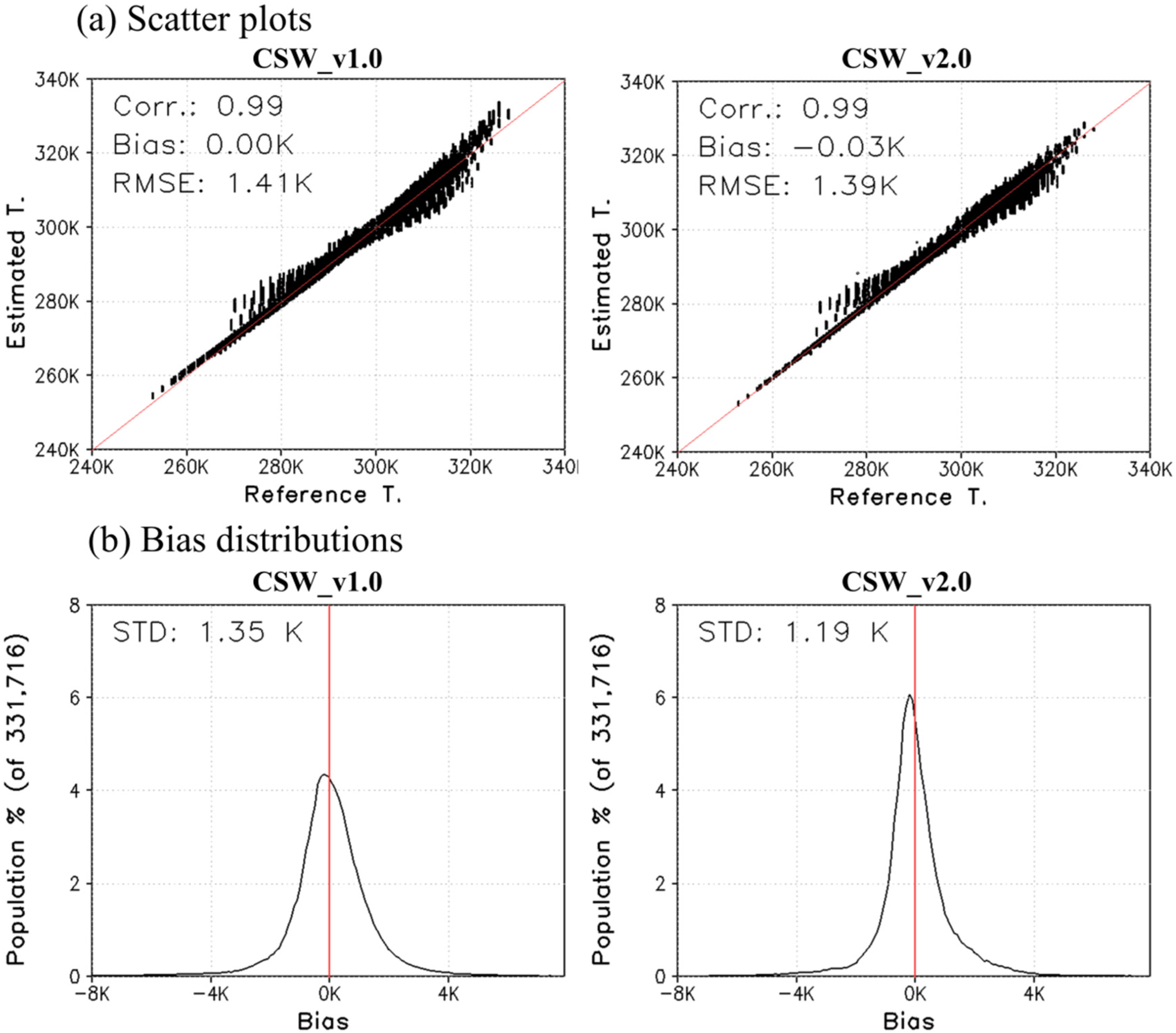
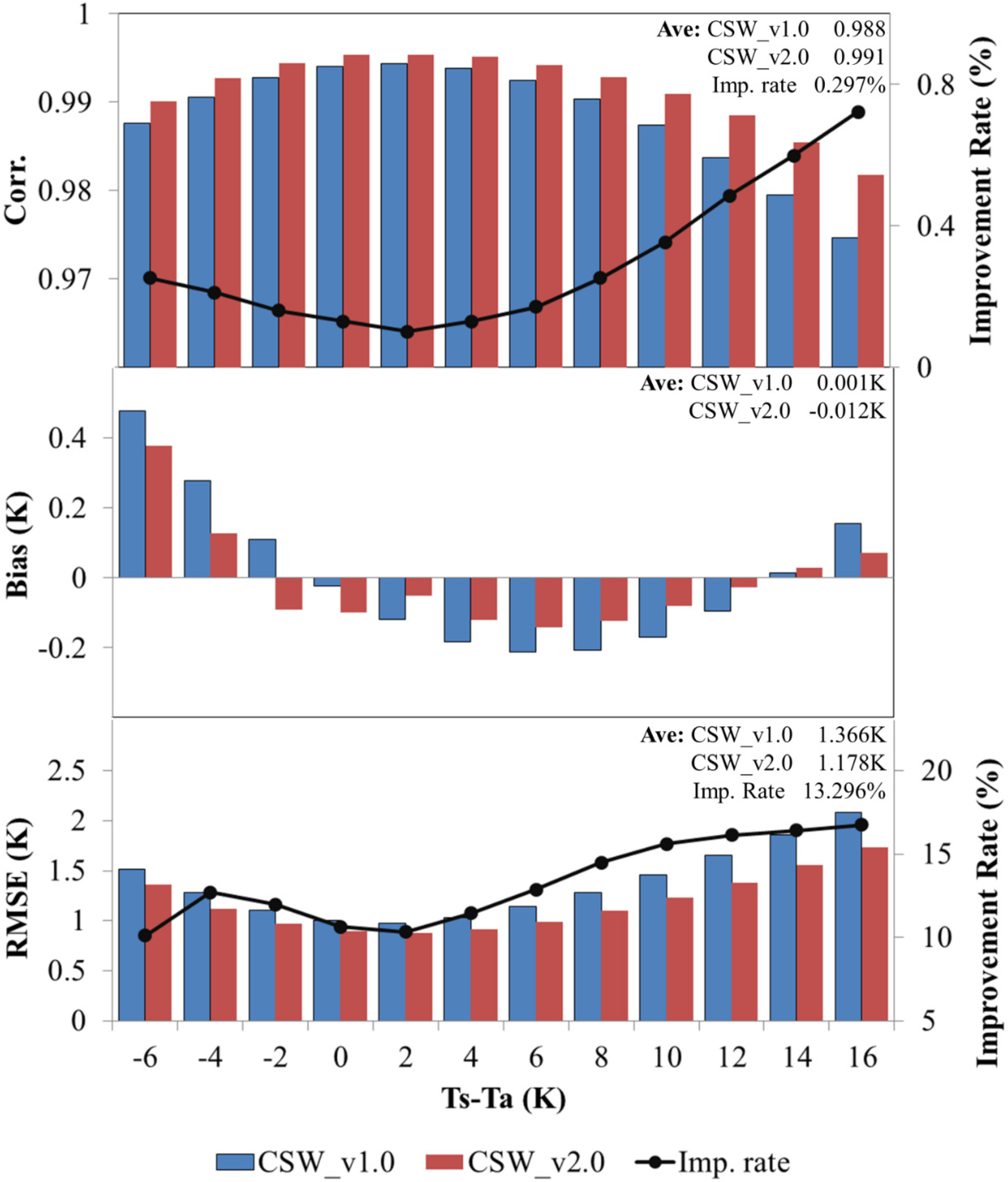
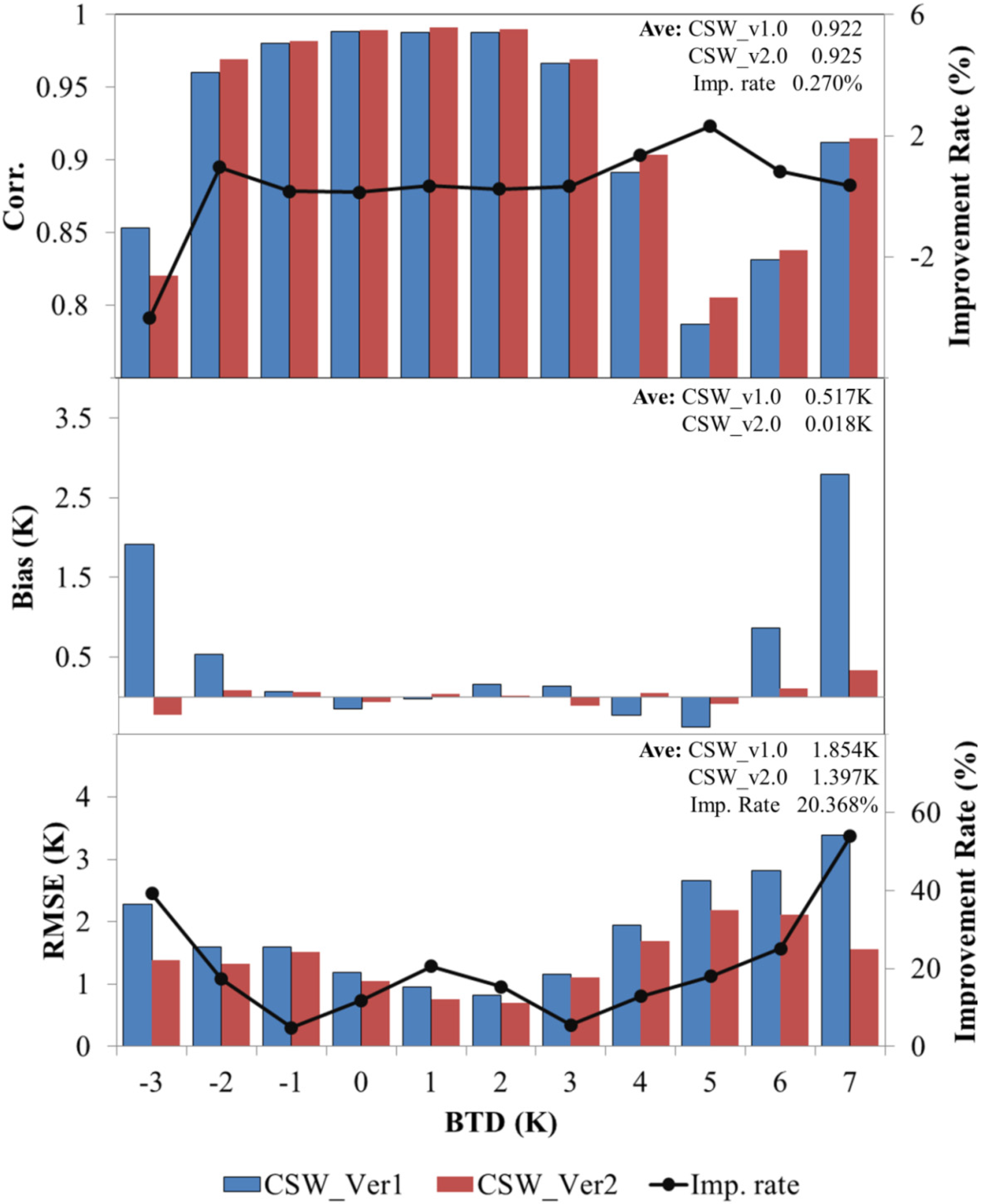
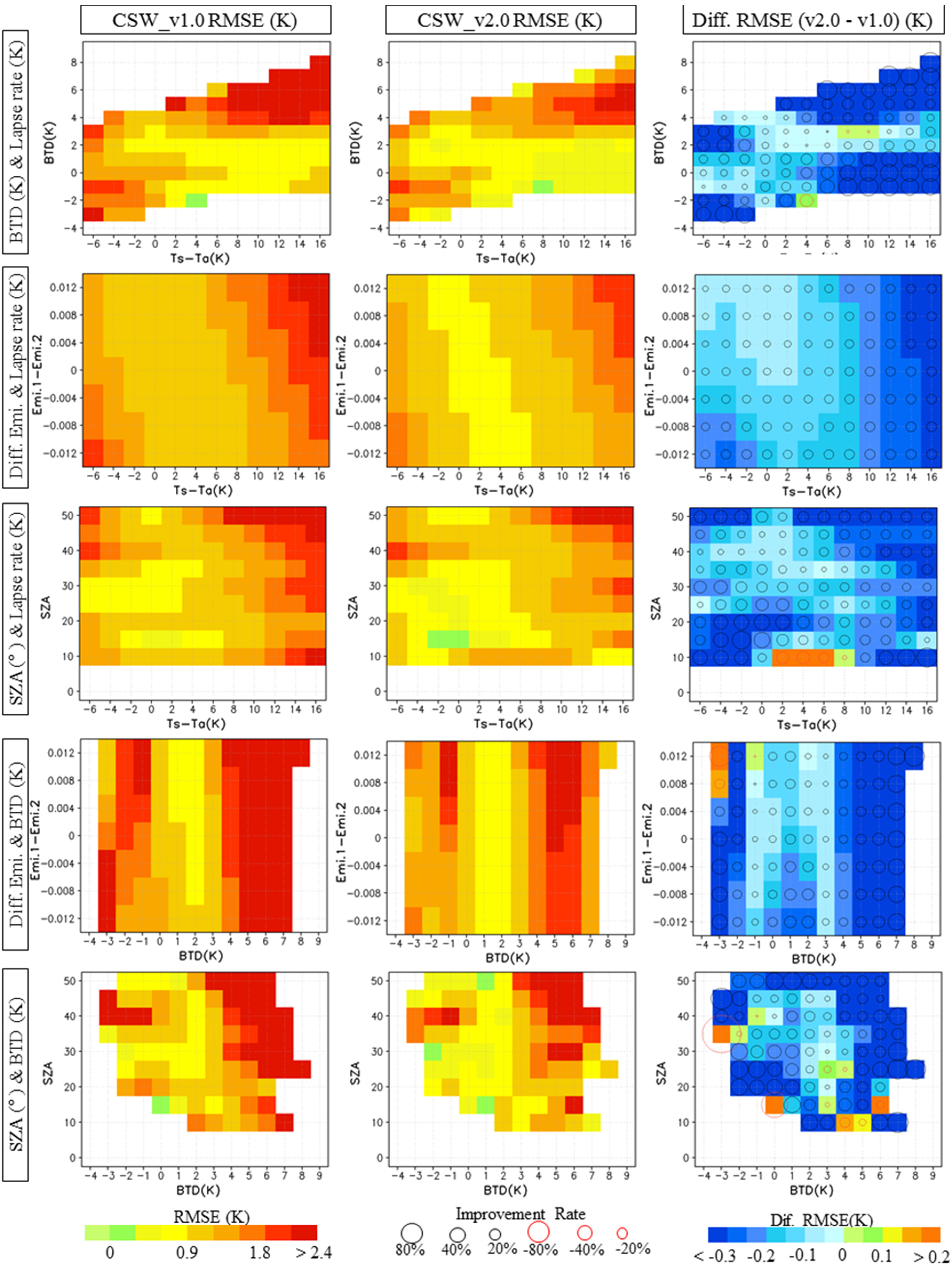
3.1. Evaluation of the CSW_v2.0 Algorithm

| −6 | −4 | −2 | 0 | 2 | 4 | 6 | 8 | 10 | 12 | 14 | 16 | |
|---|---|---|---|---|---|---|---|---|---|---|---|---|
| Cases | 27,643 | 27,643 | 27,643 | 27,643 | 27,643 | 27,643 | 27,643 | 27,643 | 27,643 | 27,643 | 27,643 | 27,643 |
| BTD | −3 | −2 | −1 | 0 | 1 | 2 | 3 | 4 | 5 | 6 | 7 | |
| Cases | 142 | 1529 | 18,297 | 51,455 | 66,442 | 67,815 | 58,758 | 40,462 | 20,951 | 5429 | 435 | |
| SZA (°) | ~10 | 10~15 | 15~20 | 20~25 | 25~30 | 30~35 | 35~40 | 40~45 | 45~50 | |||
| Cases | 924 | 3696 | 12,012 | 21,252 | 48,048 | 92,400 | 78,540 | 67,452 | 7392 | |||
| Emis. | −0.012 | −0.008 | −0.004 | 0 | 0.004 | 0.008 | 0.012 | |||||
| Cases | 47,388 | 47,388 | 47,388 | 47,388 | 47,388 | 47,388 | 47,388 |

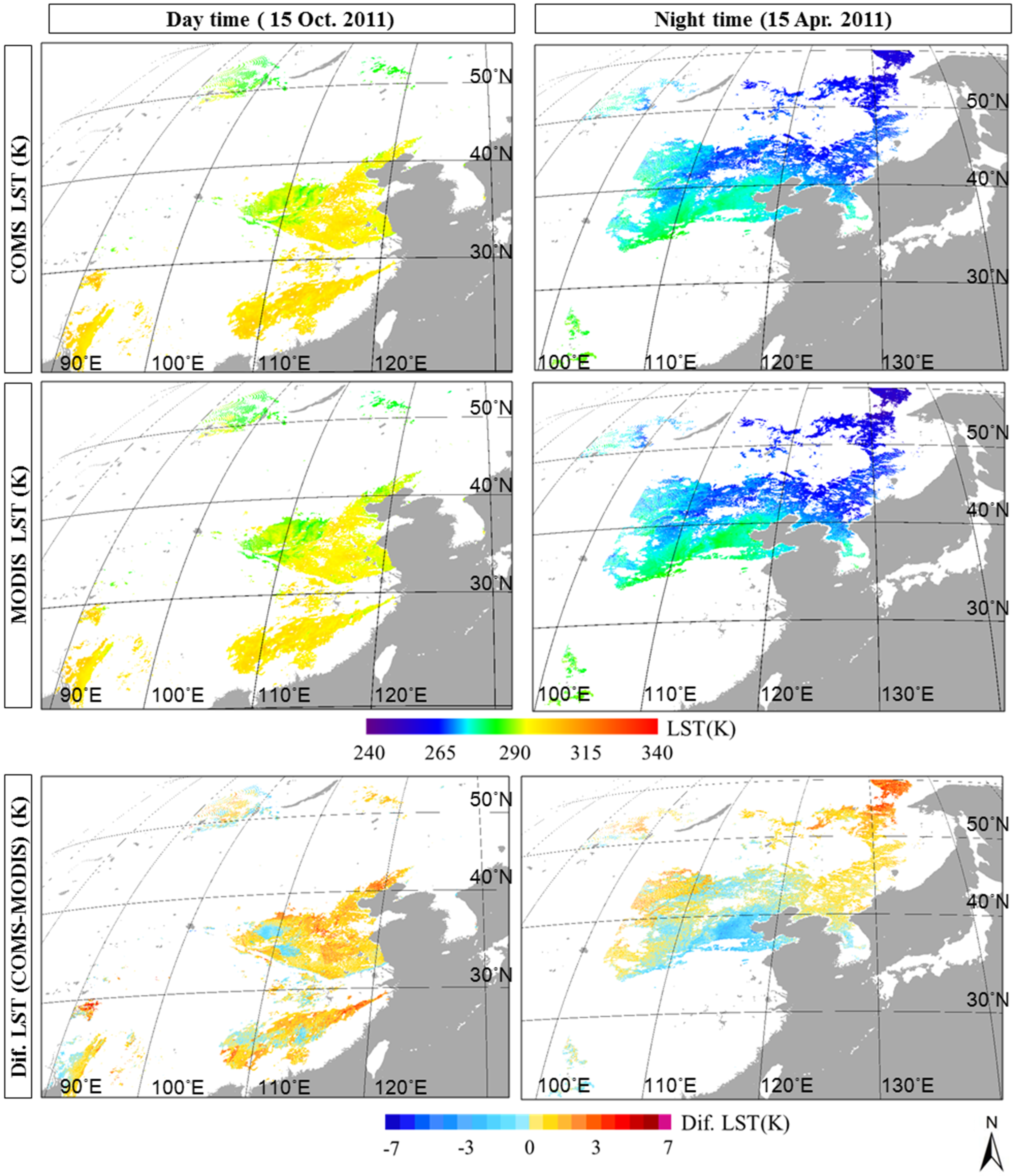
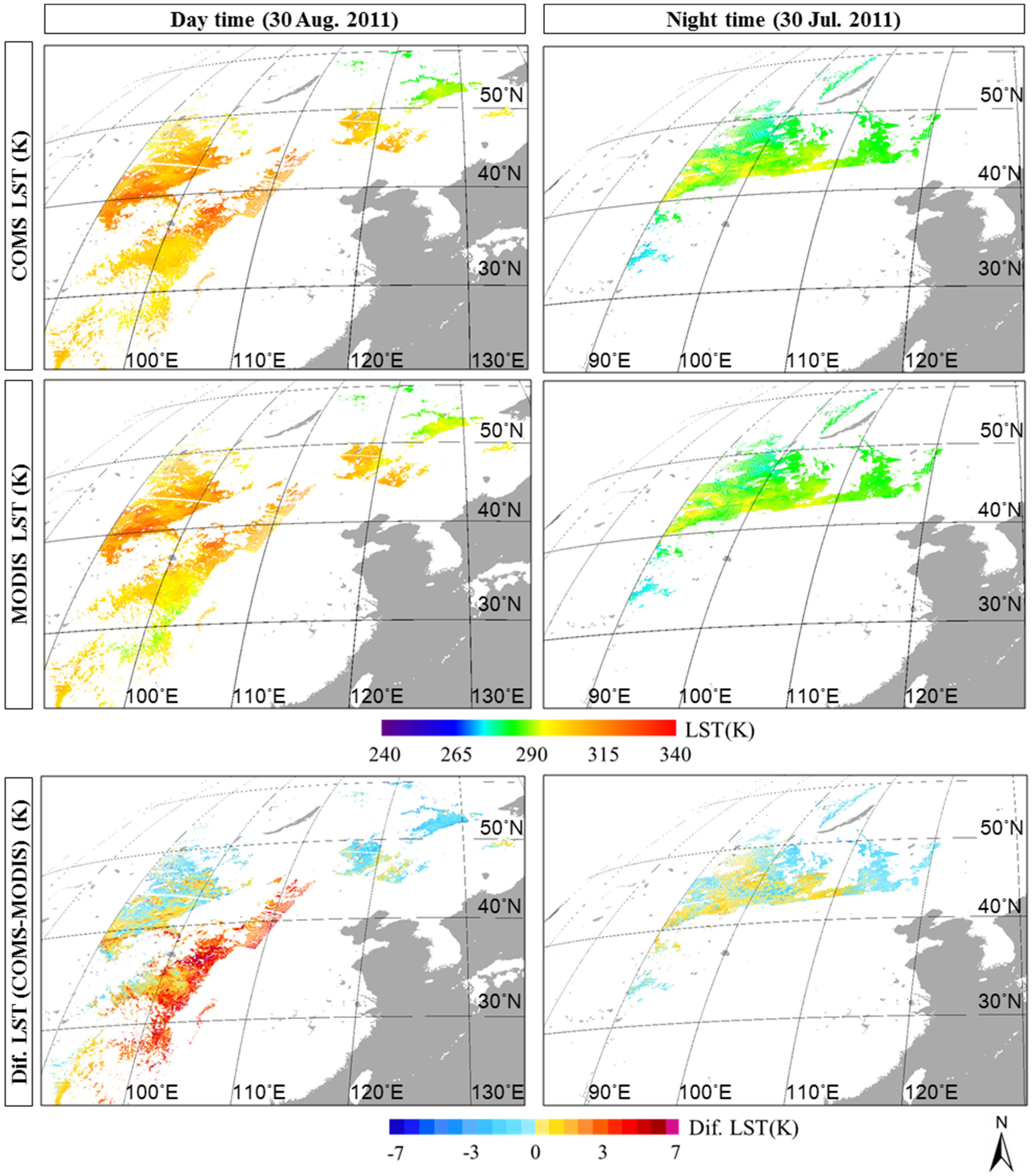
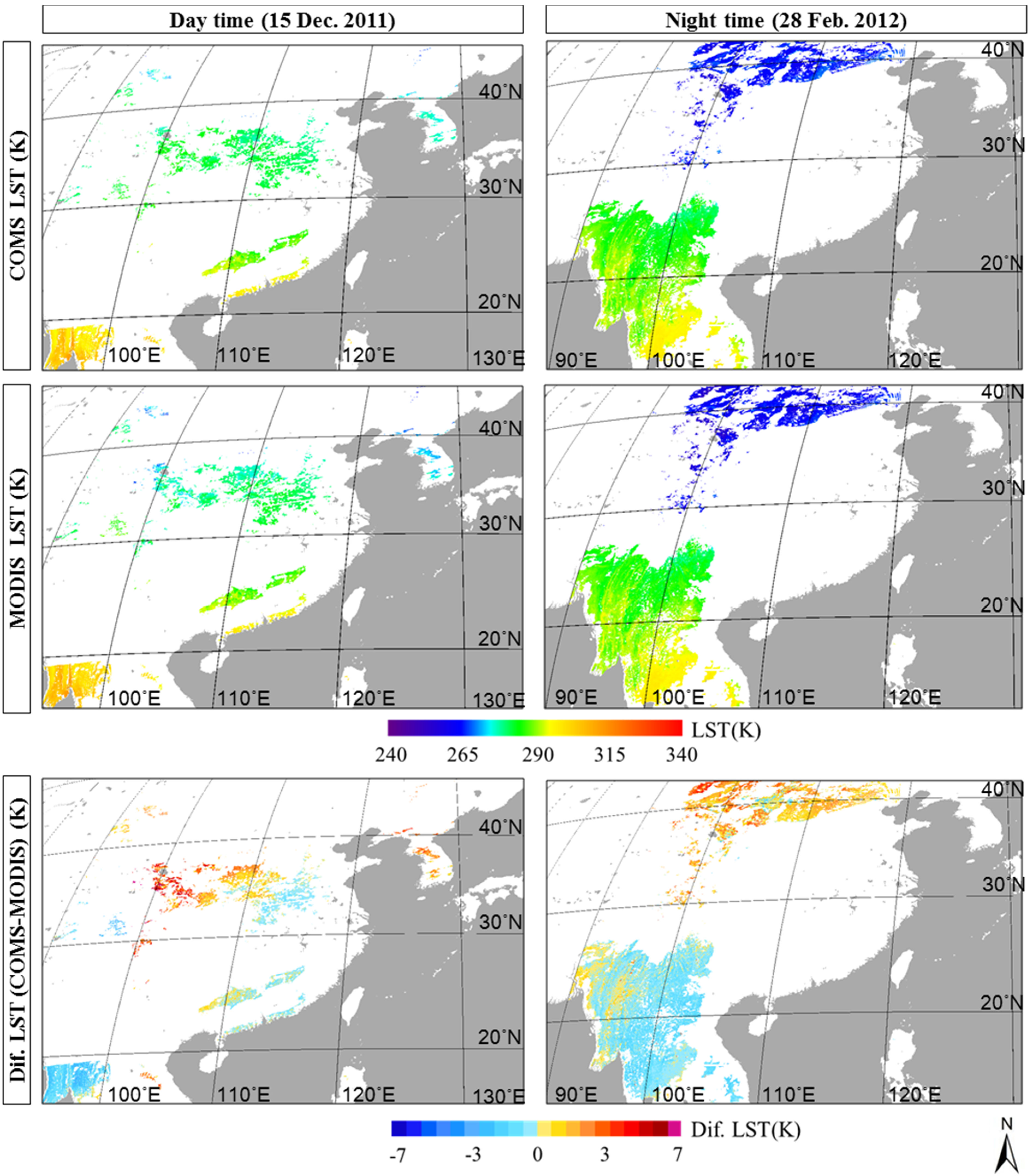
3.2. Validation of CSW_v2.0 Using MODIS LST Data


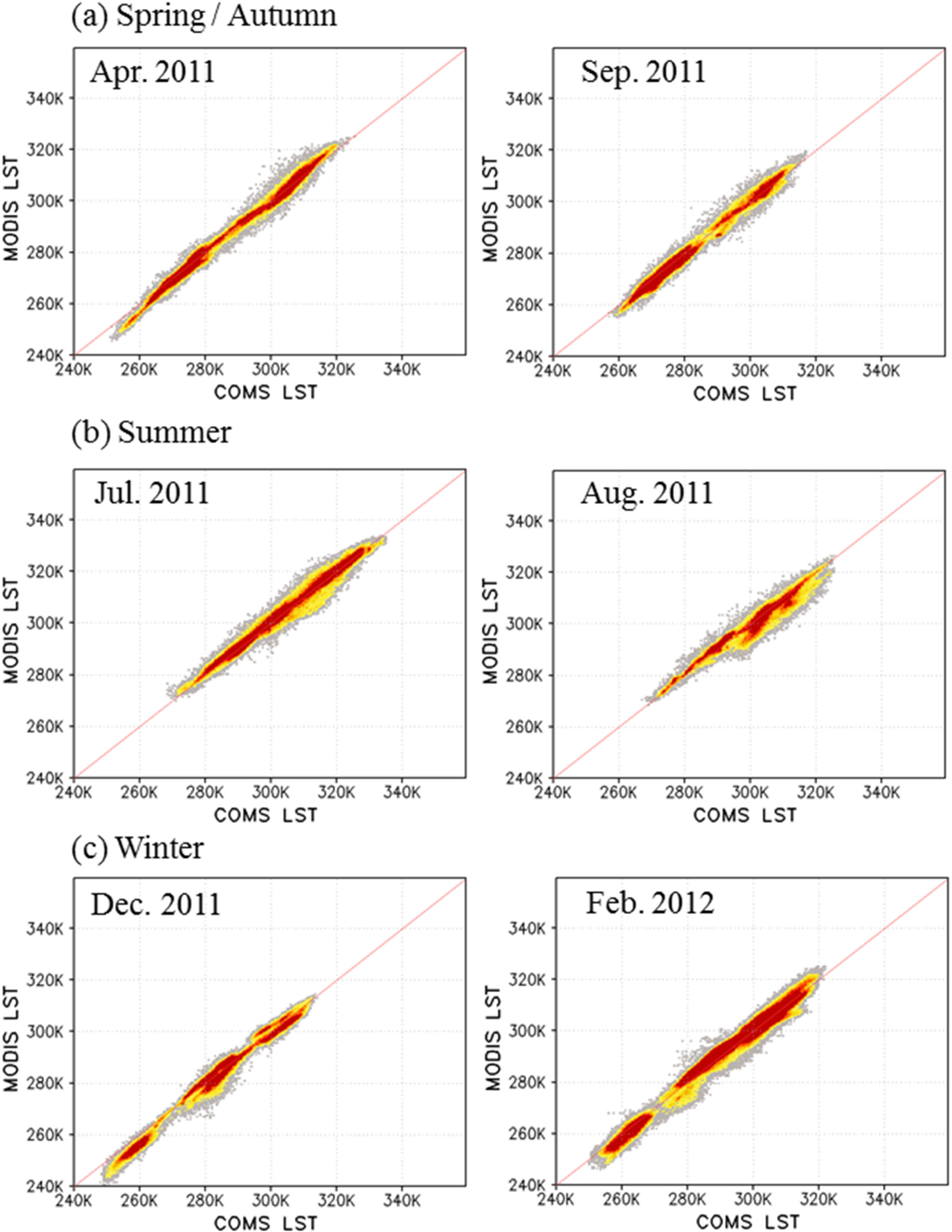
| Mon. | 4 | 5 | 6 | 7 | 8 | 9 | 10 | 11 | 12 | 1 | 2 | 3 | Ave. | |
|---|---|---|---|---|---|---|---|---|---|---|---|---|---|---|
| Corr. | Ver1 | 0.995 | 0.995 | 0.984 | 0.986 | 0.968 | 0.993 | 0.991 | 0.991 | 0.987 | 0.982 | 0.990 | 0.992 | 0.988 |
| Ver2 | 0.995 | 0.996 | 0.986 | 0.990 | 0.968 | 0.993 | 0.992 | 0.994 | 0.991 | 0.983 | 0.990 | 0.991 | 0.989 | |
| Bias (K) | Ver1 | −1.506 | −2.421 | −1.415 | −1.220 | −0.010 | −1.289 | 0.079 | −0.166 | −0.004 | −1.386 | −1.080 | −1.692 | −1.009 |
| Ver2 | 0.224 | −0.528 | 0.743 | −0.221 | 0.717 | 0.623 | 1.360 | 1.089 | 1.093 | −0.393 | −0.278 | −0.927 | 0.292 | |
| RMSE (K) | Ver1 | 2.477 | 3.056 | 2.737 | 2.735 | 3.175 | 2.075 | 1.988 | 2.136 | 2.662 | 3.126 | 2.506 | 2.681 | 2.613 |
| Ver2 | 1.854 | 1.863 | 2.016 | 2.033 | 2.883 | 1.831 | 2.134 | 2.123 | 2.573 | 2.724 | 2.323 | 2.490 | 2.237 | |
4. Summary
Acknowledgments
Author Contributions
Conflicts of Interest
References
- Noilhan, J.; Planton, S. A simple parameterization of land surface processes for meteorological models. Mon. Weather Rev. 1989, 117, 536–549. [Google Scholar] [CrossRef]
- Aires, F.; Prigent, C.; Rossow, W.; Rothstein, M. A new neural network approach including first guess for retrieval of atmospheric water vapor, cloud liquid water path, surface temperature, and emissivities over land from satellite microwave observations. J. Geophys. Res. 2001, 106, 14887–14907. [Google Scholar] [CrossRef]
- Sun, D.; Pinker, R.T. Estimation of land surface temperature from a Geostationary Operational Environmental Satellite (GOES‐8). J. Geophys. Res. 2003, 108. [Google Scholar] [CrossRef]
- Pinheiro, A.; Mahoney, R.; Privette, J.; Tucker, C. Development of a daily long term record of NOAA-14 AVHRR land surface temperature over Africa. Remote Sens. Environ. 2006, 103, 153–164. [Google Scholar] [CrossRef]
- Hachem, S.; Allard, M.; Duguay, C. Using the MODIS land surface temperature product for mapping permafrost: An application to northern Québec and Labrador, Canada. Permafr. Periglac. Process. 2009, 20, 407–416. [Google Scholar] [CrossRef]
- Benali, A.; Carvalho, A.; Nunes, J.; Carvalhais, N.; Santos, A. Estimating air surface temperature in Portugal using MODIS LST data. Remote Sens. Environ. 2012, 124, 108–121. [Google Scholar] [CrossRef]
- Guo, M.; Wang, X.; Li, J.; Yi, K.; Zhong, G.; Tani, H. Assessment of global carbon dioxide concentration using MODIS and GOSAT data. Sensors 2012, 12, 16368–16389. [Google Scholar] [CrossRef] [PubMed]
- Pal, S.; Xueref-Remy, I.; Ammoura, L.; Chazette, P.; Gibert, F.; Royer, P.; Dieudonne, E.; Dupont, J.C.; Haeffelin, M.; Lac, C.; et al. Spatio-temporal variability of the atmospheric boundary layer depth over the Paris agglomeration: An assessment of the impact of the urban heat island intensity. Atmos. Environ. 2012, 63, 261–275. [Google Scholar] [CrossRef]
- Lac, C.; Donnelly, R.P.; Masson, V.; Pal, S.; Donier, S.; Queguiner, S.; Tanguy, G.; Ammoura, L.; Xueref-Remy, I. CO2 dispersion modelling over Paris region within the CO2-MEGAPARIS project. Atmos. Chem. Phys. 2013, 13, 4941–4961. [Google Scholar] [CrossRef]
- Kustas, W.; Norman, J. Use of remote sensing for evapotranspiration monitoring over land surfaces. Hydrolog. Sci. J. 1996, 41, 495–516. [Google Scholar] [CrossRef]
- Moran, M.S.; Jackson, R.D. Assessing the spatial distribution of evapotranspiration using remotely sensed inputs. J. Environ. Qual. 1991, 20, 725–737. [Google Scholar] [CrossRef]
- Wan, Z.; Dozier, J. A generalized split-window algorithm for retrieving land-surface temperature from space. IEEE Trans. Geosci. Remote Sens. 1996, 34, 892–905. [Google Scholar] [CrossRef]
- Li, Z.-L.; Tang, B.-H.; Wu, H.; Ren, H.; Yan, G.; Wan, Z.; Trigo, I.F.; Sobrino, J.A. Satellite-derived land surface temperature: Current status and perspectives. Remote Sens. Environ. 2013, 131, 14–37. [Google Scholar] [CrossRef]
- Prata, A.; Caselles, V.; Coll, C.; Sobrino, J.; Ottle, C. Thermal remote sensing of land surface temperature from satellites: Current status and future prospects. Remote Sens. Rev. 1995, 12, 175–224. [Google Scholar] [CrossRef]
- Cristòbal, J.; Jimènez-Muñez, J.C.; Sobrino, J.A; Ninyerola, M.; Pons, X. Improvements in land surface temperature retrieval from the Landsat series thermal band using water vapor and air temperature. J. Geophys. Res. 2009, 114. [Google Scholar] [CrossRef]
- Price, J.C. Land surface temperature measurements from the split window channels of the NOAA 7 Advanced Very High Resolution Radiometer. J. Geophys. Res. 1984, 89, 7231–7237. [Google Scholar] [CrossRef]
- Kerr, Y.H.; Lagouarde, J.P.; Imbernon, J. Accurate land surface temperature retrieval from AVHRR data with use of an improved split window algorithm. Remote Sens. Environ. 1992, 41, 197–209. [Google Scholar] [CrossRef]
- Ulivieri, C.; Castronuovo, M.; Francioni, R.; Cardillo, A. A split window algorithm for estimating land surface temperature from satellites. Adv. Space Res. 1994, 14, 59–65. [Google Scholar] [CrossRef]
- Han, K.-S.; Viau, A.; Anctil, F. An analysis of GOES and NOAA derived land surface temperatures estimated over a boreal forest. Int. J. Remote Sens. 2004, 25, 4761–4780. [Google Scholar] [CrossRef]
- Suh, M.-S.; Kim, S.-H.; Kang, J.-H. A comparative study of algorithms for estimating land surface temperature from MODIS data. Kor. J. Remote Sens. 2008, 24, 65–78. [Google Scholar]
- Prata, A.; Cechet, R. An assessment of the accuracy of land surface temperature determination from the GMS-5 VISSR. Remote Sens. Environ. 1999, 67, 1–14. [Google Scholar] [CrossRef]
- Peres, L.F.; DaCamara, C.C. Land surface temperature and emissivity estimation based on the two-temperature method: Sensitivity analysis using simulated MSG/SEVIRI data. Remote Sens. Environ. 2004, 91, 377–389. [Google Scholar] [CrossRef]
- Inamdar, A.K.; French, A. Disaggregation of GOES land surface temperatures using surface emissivity. Geophys. Res. Lett. 2009, 36. [Google Scholar] [CrossRef]
- Pinker, R.T.; Sun, D.; Hung, M.-P.; Li, C.; Basara, J.B. Evaluation of satellite estimates of land surface temperature from GOES over the United States. J. Appl. Meteorol. Climatol. 2009, 48, 167–180. [Google Scholar] [CrossRef]
- Cho, A.-R.; Suh, M.-S. Evaluation of land surface temperature operationally retrieved from Korean geostationary satellite (COMS) data. Remote Sens. 2013, 5, 3951–3970. [Google Scholar] [CrossRef]
- Sobrino, J.; Romaguera, M. Land surface temperature retrieval from MSG1-SEVIRI data. Remote Sens. Environ. 2004, 92, 247–254. [Google Scholar] [CrossRef]
- Kalma, J.D.; McVicar, T.R.; McCabe, M.F. Estimating land surface evaporation: A review of methods using remotely sensed surface temperature data. Surv. Geophys. 2008, 29, 421–469. [Google Scholar] [CrossRef]
- Dousset, B.; Gourmelon, F.; Laaidi, K.; Zeghnoun, A.; Giraudet, E.; Bretin, P.; Mauri, E.; Vandentorren, S. Satellite monitoring of summer heat waves in the Paris metropolitan area. Int. J. Climatol. 2011, 31, 313–323. [Google Scholar] [CrossRef]
- Peng, S.; Piao, S.; Ciais, P.; Friedlingstein, P.; Ottle, C.; Bréon, F.M.; Nan, H.; Zhou, L.; Myneni, R.B. Surface urban heat island across 419 global big cities. Environ. Sci. Technol. 2011, 46, 696–703. [Google Scholar] [CrossRef] [PubMed]
- Roth, M. Effect of cities on local climates. In Proceedings of the 2002 Workshop of IGES/APN Mega-City Project, Kitakyushu, Japan, 23–25 January 2002; pp. 1–13.
- Choi, Y.-Y.; Suh, M.-S.; Park, K.-H. Assessment of surface urban heat islands over three megacities in East Asia using land surface temperature data retrieved from COMS. Remote Sens. 2014, 6, 5852–5867. [Google Scholar] [CrossRef]
- Kerr, Y.H.; Lagouarde, J.P.; Nerry, F.; Ottlé, C. Land surface temperature retrieval techniques and applications. In Thermal Remote Sensing in Land Surface Processes; CRC Press: Boston, MA, USA, 2004; pp. 33–109. [Google Scholar]
- Dash, P. Land Surface Temperature and Emissivity Retrieval from Satellite Measurements. Available online: http://d-nb.info/97521960x/34/ (accessed on 9 October 2014).
- Behrendt, A.; Pal, S.; Aoshima, F.; Bender, M.; Blyth, A.; Corsmeier, U.; Cuesta, J.; Dick, G.; di Girolamo, P; Dominger, M.; et al. Observation of convection initiation processes with a suite of state-of-the-art research instruments during COPS IOP8b. Q. J. R. Meteorol. Soc. 2011, 137, 81–100. [Google Scholar] [CrossRef]
- Goïta, K.; Royer, A.; Bussières, N. Crseharacterization of land surface thermal structure from NOAA-AVHRR data over a northern ecosystem. Remote Sens. Environ. 1997, 60, 282–298. [Google Scholar] [CrossRef]
- Sobrino, J.; Raissouni, N. Toward remote sensing methods for land cover dynamic monitoring: Application to Morocco. Int. J. Remote Sens. 2000, 21, 353–366. [Google Scholar] [CrossRef]
- Sobrino, J.; Sòria, G.; Prata, A. Surface temperature retrieval from Along Track Scanning Radiometer 2 data: Algorithms and validation. J. Geophys. Res.: Atmos. 2004, 109, D11101. [Google Scholar] [CrossRef]
- Sòria, G.; Sobrino, J.A. ENVISAT/AATSR derived land surface temperature over a heterogeneous region. Remote Sens. Environ. 2007, 111, 409–422. [Google Scholar] [CrossRef]
- National Meteorological Satellite Center (NMSC). Available online: http://nmsc.kma.go.kr (accessed on 9 October 2014).
- Valor, E.; Caselles, V. Mapping land surface emissivity from NDVI: Application to European, African, and South American areas. Remote Sens. Environ. 1996, 57, 167–184. [Google Scholar] [CrossRef]
- Thermodynamic Initial Guess Retrieval (TIGR). Available online: http://ara.abct.lmd.polytechnique.fr/index.php?page=tigr (accessed on 9 October 2014).
- Wan, Z. New refinements and validation of the MODIS land-surface temperature/emissivity products. Remote Sens. Environ. 2008, 112, 59–74. [Google Scholar] [CrossRef]
- Frey, C.M.; Kuenzer, C.; Dech, S. Quantitative comparison of the operational NOAA-AVHRR LST product of DLR and the MODIS LST product V005. Int. J. Remote Sens. 2012, 33, 7165–7183. [Google Scholar] [CrossRef]
- Berk, A.; Anderson, G.P.; Acharya, P.K.; Chetwynd, J.H.; Bernstein, L.S.; Shettle, E.P.; Matthew, M.W.; Adler-Golden, S.M. MODTRAN4 Users’s Mannual; Air Force Research Laboratory: Hanscom AFB, MA, USA, 1999. [Google Scholar]
© 2015 by the authors; licensee MDPI, Basel, Switzerland. This article is an open access article distributed under the terms and conditions of the Creative Commons Attribution license (http://creativecommons.org/licenses/by/4.0/).
Share and Cite
Cho, A.-R.; Choi, Y.-Y.; Suh, M.-S. Improvements of a COMS Land Surface Temperature Retrieval Algorithm Based on the Temperature Lapse Rate and Water Vapor/Aerosol Effect. Remote Sens. 2015, 7, 1777-1797. https://doi.org/10.3390/rs70201777
Cho A-R, Choi Y-Y, Suh M-S. Improvements of a COMS Land Surface Temperature Retrieval Algorithm Based on the Temperature Lapse Rate and Water Vapor/Aerosol Effect. Remote Sensing. 2015; 7(2):1777-1797. https://doi.org/10.3390/rs70201777
Chicago/Turabian StyleCho, A-Ra, Youn-Young Choi, and Myoung-Seok Suh. 2015. "Improvements of a COMS Land Surface Temperature Retrieval Algorithm Based on the Temperature Lapse Rate and Water Vapor/Aerosol Effect" Remote Sensing 7, no. 2: 1777-1797. https://doi.org/10.3390/rs70201777