Automation Aspects for the Georeferencing of Photogrammetric Aerial Image Archives in Forested Scenes

Abstract

Photogrammetric aerial film image archives are scanned into digital form in many countries. These data sets offer an interesting source of information for scientists from different disciplines. The objective of this investigation was to contribute to the automation of a generation of 3D environmental model time series when using small-scale airborne image archives, especially in forested scenes. Furthermore, we investigated the usability of dense digital surface models (DSMs) generated using these data sets as well as the uncertainty propagation of the DSMs. A key element in the automation is georeferencing. It is obvious that for images captured years apart, it is essential to find ground reference locations that have changed as little as possible. We studied a 68-year-long aerial image time series in a Finnish Karelian forestland. The quality of candidate ground locations was evaluated by comparing digital DSMs created from the images to an airborne laser scanning (ALS)-originated reference DSM. The quality statistics of DSMs were consistent with the expectations; the estimated median root mean squared error for height varied between 0.3 and 2 m, indicating a photogrammetric modelling error of 0.1‰ with respect to flying height for data sets collected since the 1980s, and 0.2‰ for older data sets. The results show that of the studied land cover classes, “peatland without trees” changed the least over time and is one of the most promising candidates to serve as a location for automatic ground control measurement. Our results also highlight some potential challenges in the process as well as possible solutions. Our results indicate that using modern photogrammetric techniques, it is possible to reconstruct 3D environmental model time series using photogrammetric image archives in a highly automated way.

1. Introduction

Aerial imagery has been utilised since the beginning of the 20th century as a basic data source for maps. Historical aerial image film archives are now scanned and offered for users in many countries with varying levels of coverage and at varying spatial and temporal resolutions [1,2]. Use of an historical data series has been an effective approach to understand cause–effect relationships in the past, and such data series offers a means for using that information to improve projections about the future. For example, such time series data can be used to measure forest growth and monitor the dynamics of forest disturbance [3,4]. The potential of historical aerial images has also been demonstrated with respect to vegetation change [5], contamination detection [6], long-term biotope changes [7], land cover changes [8,9], watershed studies [10], archaeology [11], glacier studies [12], cadastral mapping of forestlands [13] and climatic studies [14].

Recently, new innovations have been achieved in photogrammetric processing technologies. In particular, image matching technologies are nowadays capable of producing high quality dense point clouds that are competitive or complementary to laser scanning [15,16,17,18]. Our expectation is that modern photogrammetric techniques enable reconstructions of even countrywide historical three dimensional (3D) environmental models produced from stereoscopic images.

One major challenge in the production of a time series is accurate georeferencing of the images. Modern, state-of-the-art, photogrammetric, large-format imaging systems offer highly accurate and automated georeferencing based on a directly measured sensor trajectory using accurate GNSS/IMU-systems (Global Navigation Satellite System, Inertial Measurement Unit), accurate system calibration and automated image matching. In the case of scanned historical film data, camera calibration information as well as adequate approximate exterior orientations are often missing; thus, a sufficient number of ground control points (GCPs) is required to tie the images to the ground reference system.

Korpela [3] showed the possibility of using post-positioned GCPs, immobile tie points and direct georeferencing to better orient an image time series. The selection of the points was based completely on visual interactive interpretation. In the study, rocks, stones and the roofs of buildings appeared to be the longest-lasting multi-temporal tie points. Korpela [3] concluded that it is difficult to identify immobile multi-temporal tie points in a forest environment, especially with small-scale images. For matching different images, feature-based methods are worth mentioning. Vassilaki et al. [19] compared linear features and GCPs as ground control and found the former to perform better.

Véga and St-Onge [4] used an aerial imagery time series for a period of 58 years and reconstructed forest canopy height growth. They used ALS-derived ground height for the canopy height model (CHM) generated from photogrammetric digital surface models (DSMs). They discovered that the CHMs derived from the historical aerial imagery were only slightly less accurate than the historical field data. However, the quality of the remote sensing estimates was sufficient for a variety of forest dynamics studies. With their method, the prediction of plot-wise mean dominant height was done manually. The other phases of the procedure were automated.

Ma [20] studied the use of up to third-order rational function models (RFMs) in the orthorectification of historical aerial photographs and discovered that of the studied models, the linear RFM is the optimal choice for historical aerial photographs, especially when accuracy and the number of GCPs are limited. Aguilar et al. [21] reported in their study of self-calibration accuracy that for historical aerial photographs, non-systematic errors might be greater than systematic errors and the self-calibration results cannot be transferred to other image sets obtained with the same camera.

Borgogno Mondino and Chiabrando [22] tested different scenarios for aerial triangulation using aerial time series, namely “single block bundle adjustment SBBA”, “single block sequential bundle adjustment SBSBA” and “multi-temporal block bundle adjustment MTBBA”. In their study, SBBA meant tying and adjusting each block to the reference block separately using the same GCPs whenever possible. Further, with SBSBA one image block is oriented with GCPs and the rest of the image series are tied to that block. With the MTBBA approach, the time series is adjusted simultaneously using several common GCPs. The MTBBA approach was found to be the most accurate [22].

Increased quality is to be expected when using more modern imaging systems because of the continuous progress in the geometric performance of the photogrammetric cameras. For example, the radial distortion of the Zeiss PLEOGON 5.6/153 lens—introduced in 1955—was below 5 µm compared to it having been below 50 µm with the Zeiss TOPOGON 6.3/100 lens introduced in 1932 [23]. As for the Wild Heerbrugg cameras, the RC10A differed from its predecessor, the RC10, in terms of microprocessor control [24]. Forward motion compensation (FMC) was included in the RC20 model [24]. Hildebrand [25] has described the Wild lens design background and enhanced performance of the newer model. Schlienger et al. [26] listed the performance progress of Leica f_150mm and f_300mm lenses; both lenses constituted very big steps forwards in terms of area weighted average resolution (AWAR) in 1978 (15/4 UAG), 1992 (30/4 NATS) and 1995 (15/4 UAG-S). The achievement of the Leica S lens generation, although not used in this investigation, was that it offered full optical performance at a maximum aperture of f:4 [26]. More details about the camera technology can be found in studies by Schwidefsky [27], Cimerman and Tomašegović [28], Slama et al. [29], and Hobbie [23].

Since the majority of historical aerial images have been captured on film, it should be noted that the major types of plastic films are cellulose nitrate, cellulose acetate and polyester [30]. Eastman Kodak, which is the only manufacturer that has provided dates for nitrate film production, discontinued cellulose nitrate aerial films in 1942 [31,32]. Polyester films are chemically more stable than cellulosic films [30]. The time period for aerial polyester-based films began in the 1960s, and polyester films were used, e.g., in the American Corona project [30,33,34]. Brandes [35] mentions anti-static properties, the elimination of impurities larger than 10 µm and the double-sided coating of modern Agfa polyester film base material; all are important when considering the use of digitized images. Anti-staticity aims at avoidance of dust, which is harmful for the image quality. Elimination of too large impurities, and on the other hand aspiration to lower granularity are essential, when using small scanning pixel sizes. Double-sided coating enhances film flatness during scanning, but the back coating also gives protection against scratches.

The main objective of this study was to contribute to the automation of georeferencing for aerial image archives, in particular to find and evaluate stable ground control locations for image orientation that could be utilised for the semi-automated or automated processing of 1 m ground sample distance (GSD) orthophoto and digital surface model (DSM) time series. In addition, our objective was to assess the usability potential of DSMs created from old aerial photographs as well as to study the uncertainty propagation of the DSM generation process. Our target area was the boreal forest biome and we focused on small-scale photogrammetric image archives suitable for creating countrywide time series. We also considered the integration of ALS data with historical time series data processing and analysis, and we utilised the existing national topographic database in our work. Our study concentrates on image time series orientation from the standpoint of evincing automation prerequisites and is motivated by earlier studies by Korpela [3] and Véga and St-Onge [4]. Although they realised the importance of ground object classification with respect to GCPs, they did not automate the selection process of GCP candidates on the basis of map object classification.

The study area, data sets and processing and analysis methods are presented in Section 2. We provide the results of the investigation in Section 3 and a discussion in Section 4.

2. Study Area, Data Sets and Analysis Methods

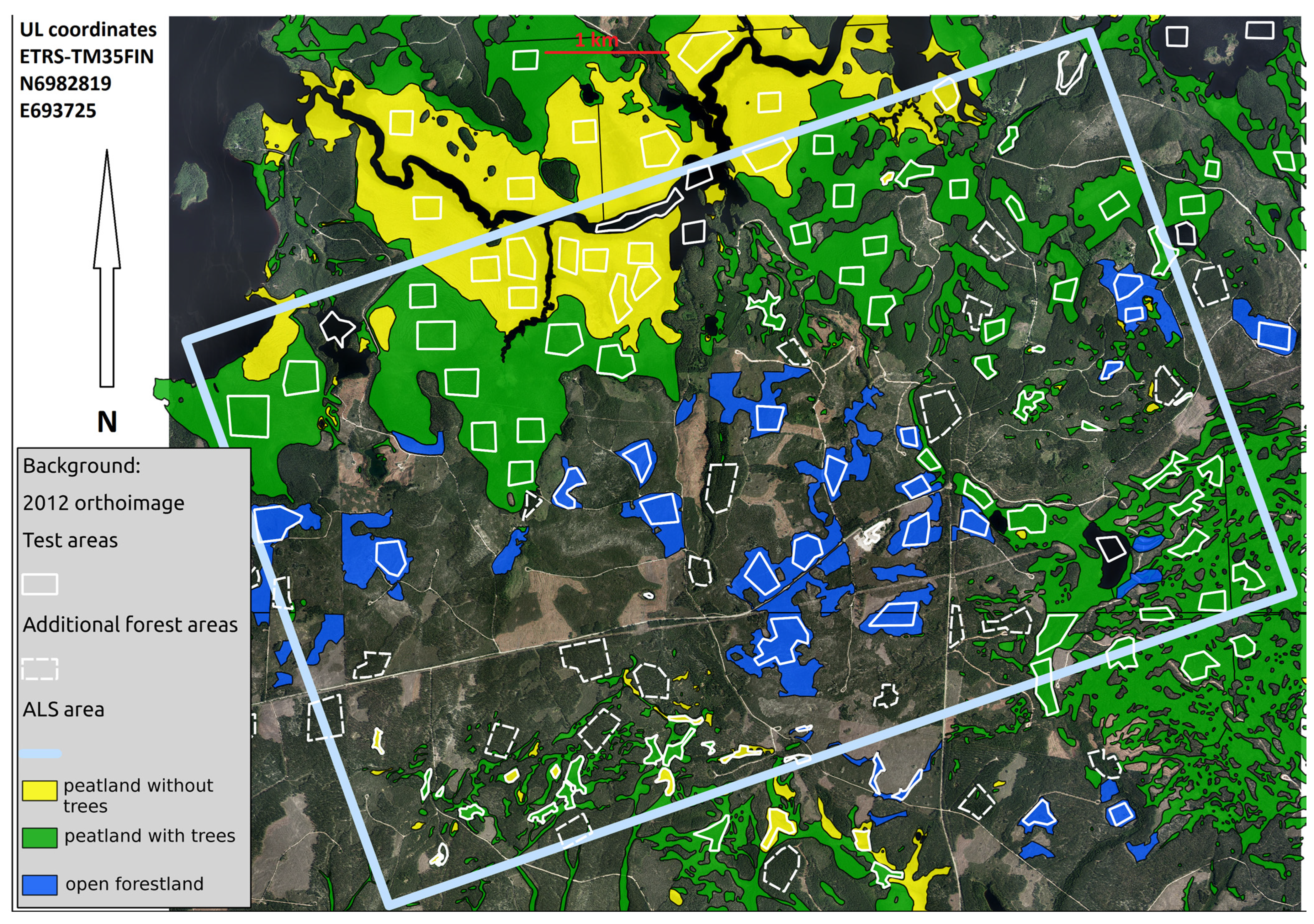
Our study site was located in the municipality of Ilomantsi, in eastern Finland (62°53′N, 30°54′E). The mean elevation is approximately 170 m above sea level and the topography is mainly flat, rolling towards the north. The main land cover classes present in the topographic database on the study area were “peatland without trees”, “peatland with trees” and “open forestland”. Other classes that were present included “lake water”, “wetland” and “rocky ground”. The national Topographic Database does not include the forest polygons. The study area and the land cover classes are shown in Figure 1.

2.1. Airborne Data Sets

The airborne images used in this investigation cover a time period of 68 years, from 1944 to 2012 (Table 1). They were originally collected for the purposes of national-level topographic mapping by the National Land Survey of Finland (NLS) (data sets from 1977, 1983, 1991, 2003 and 2012) and the Finnish Defence Intelligence Agency (data sets from 1944, 1959 and 1965). The imaging technology has changed greatly over the years (Table 2). Until 2009, film cameras were used in image data collection; since then, digital cameras have been used. The film images were mostly panchromatic and collected at altitudes of 4–8 km. The images from 1991 were collected using false colour infrared film, and the digital images were multispectral data with red, green, blue and near-infrared spectral sensitivities. Airborne images were collected in June and July, and thus during leaf-on conditions. Since the images are utilised in digital format, the NLS is currently scanning the entire historical film image archive in Finland. Since the year 2000, they have used Leica DSW photogrammetric scanners in the scanning process. The scanning pixel size of the film images used in this study was 15 µm or 20 µm, depending on the vintage. The GSDs varied from 0.45 m to 0.88 m.

Figure 1. The Palokangas study area in Ilomantsi. The land cover polygons from the National Land Survey of Finland’s (NLS) Topographic Database are shown over a 2012 orthophoto. The ALS coverage is shown as a light blue, tilted rectangle on top of the image. The test patches outlined in white. Open data used for image orientation, © NLS, Colour Orthophoto and Elevation Model 10 m, October 2013. Open data used for vector overlay, © NLS, The Topographic Database and Colour Orthophoto, September 2014. Licences for the NLS data, [36].

Figure 1. The Palokangas study area in Ilomantsi. The land cover polygons from the National Land Survey of Finland’s (NLS) Topographic Database are shown over a 2012 orthophoto. The ALS coverage is shown as a light blue, tilted rectangle on top of the image. The test patches outlined in white. Open data used for image orientation, © NLS, Colour Orthophoto and Elevation Model 10 m, October 2013. Open data used for vector overlay, © NLS, The Topographic Database and Colour Orthophoto, September 2014. Licences for the NLS data, [36].

The ALS data set was acquired in October 2008 using a Leica ALS50-II SN058 laser scanner (Leica Geosystems AG, Heerbrugg, Switzerland). The flying altitude was 500 m at a speed of 80 knots, with a field of view of 30 degrees, a pulse rate of 150 kHz, a scanning rate of 52 Hz and a ground-level laser footprint size of 0.11 m. The density of the pulses returned was approximately 20 pulses per m².

The ALS data form the basis for the analysis by providing the elevation of the ground. The photogrammetric DSM area was 68.8 km², but some of the image blocks covered it only partly. The ALS area coverage consisted of a rotated quadrangle inside the photogrammetric area, covering 37.8 km². Further details on the image blocks are given in Table 1 and Table 2.

Table 1. Details of the image blocks used in this investigation. FH = Flying height above the average ground level; FD = major flight direction: NS = North-South, EW = East-West; Overlaps: p = forward overlap, q = side overlap.

Flight Number	Date of Flight	Scale	FH (km)	FD	Overlaps p; q (%)	GSD (m)	Camera	Film
1944123	13.7.1944	1:30K	6.125	EW	67; 38	0.45	Zeiss-Aerotopograph RMK HS 1824	Nitrate
195915	22.7.1959	1:40K	4.145	NS	67; 36	0.62	Zeiss-Aerotopograph RMK HS 1818	Kodak Super XX
195920	27.7.1959	1:40K	4.000	NS		0.61	Zeiss-Aerotopograph RMK HS 1818	Gevaert Gevapan 33
196507	4.6.1965	1:60K	8.940	NS	79; -	0.88	Carl Zeiss Oberkochen RMK 15/23	Unknown
1977192	11.6.1977	1:31K	6.670	EW	59; 39	0.47	Wild Heerbrugg RC10	Unknown
1983235	5.6.1983	1:31K	6.440	EW	63; 25	0.45	Wild Heerbrugg RC10A	Unknown
1991422A	29.7.1991	1:31K	6.710	EW	70; 22	0.63	Wild Heerbrugg RC20	Unknown
03133A	7.6.2003	1:31K	4.765	NS	65; 29	0.62	Wild Heerbrugg RC20	Unknown
03133B	16.7.2003	1:31K	4.750	NS		0.62	Wild Heerbrugg RC20	Unknown
20121519B	14.6.2012	1:75K	7.450	NS	60; 30	0.45	Vexcel Imaging UltraCam Xp	Digital sensor

Table 1. Details of the image blocks used in this investigation. FH = Flying height above the average ground level; FD = major flight direction: NS = North-South, EW = East-West; Overlaps: p = forward overlap, q = side overlap.

Flight Number	Date of Flight	Scale	FH (km)	FD	Overlaps p; q (%)	GSD (m)	Camera	Film
1944123	13.7.1944	1:30K	6.125	EW	67; 38	0.45	Zeiss-Aerotopograph RMK HS 1824	Nitrate
195915	22.7.1959	1:40K	4.145	NS	67; 36	0.62	Zeiss-Aerotopograph RMK HS 1818	Kodak Super XX
195920	27.7.1959	1:40K	4.000	NS		0.61	Zeiss-Aerotopograph RMK HS 1818	Gevaert Gevapan 33
196507	4.6.1965	1:60K	8.940	NS	79; -	0.88	Carl Zeiss Oberkochen RMK 15/23	Unknown
1977192	11.6.1977	1:31K	6.670	EW	59; 39	0.47	Wild Heerbrugg RC10	Unknown
1983235	5.6.1983	1:31K	6.440	EW	63; 25	0.45	Wild Heerbrugg RC10A	Unknown
1991422A	29.7.1991	1:31K	6.710	EW	70; 22	0.63	Wild Heerbrugg RC20	Unknown
03133A	7.6.2003	1:31K	4.765	NS	65; 29	0.62	Wild Heerbrugg RC20	Unknown
03133B	16.7.2003	1:31K	4.750	NS		0.62	Wild Heerbrugg RC20	Unknown
20121519B	14.6.2012	1:75K	7.450	NS	60; 30	0.45	Vexcel Imaging UltraCam Xp	Digital sensor

Table 2. Camera information. f = focal length; FOV = image field of view at format corner; FMC = Forward motion compensation.

Camera Name	Lens f (mm)	Maximum Aperture	Image Format (cm)	± FOV (°)	FMC	Lab. Calibration	N Fiducials
Zeiss-Aerotopograph RMK HS 1824	ORTHOMETAR; 204.53	4.5	18 × 18	32	No	NA	4
Zeiss-Aerotopograph RMK HS 1818	TOPOGON; 100.00	6.3	18 × 18	52	No	NA	4
Carl Zeiss Oberkochen RMK 15/23	PLEOGON; 152.45	5.6	23 × 23	37	No	1 January 1963	4
Wild Heerbrugg RC10	NAG II 213.57	4	23 × 23	28	No	23 February 1976	4
Wild Heerbrugg RC10A	NAG IIA 214.08	4	23 × 23	28	No	10 February 1983	4
Wild Heerbrugg RC20	NAGA-F 214.10	4	23 × 23	28	Yes	5 May 1990	8
Wild Heerbrugg RC20	UAGA-F 153.03	4	23 × 23	37	Yes	21 January 2002	8
Vexcel Imaging UltraCam Xp	100.50	5.6 Pan 4 MS	6.786 × 10.386	32	Yes	18 October 2011	No

Table 2. Camera information. f = focal length; FOV = image field of view at format corner; FMC = Forward motion compensation.

Camera Name	Lens f (mm)	Maximum Aperture	Image Format (cm)	± FOV (°)	FMC	Lab. Calibration	N Fiducials
Zeiss-Aerotopograph RMK HS 1824	ORTHOMETAR; 204.53	4.5	18 × 18	32	No	NA	4
Zeiss-Aerotopograph RMK HS 1818	TOPOGON; 100.00	6.3	18 × 18	52	No	NA	4
Carl Zeiss Oberkochen RMK 15/23	PLEOGON; 152.45	5.6	23 × 23	37	No	1 January 1963	4
Wild Heerbrugg RC10	NAG II 213.57	4	23 × 23	28	No	23 February 1976	4
Wild Heerbrugg RC10A	NAG IIA 214.08	4	23 × 23	28	No	10 February 1983	4
Wild Heerbrugg RC20	NAGA-F 214.10	4	23 × 23	28	Yes	5 May 1990	8
Wild Heerbrugg RC20	UAGA-F 153.03	4	23 × 23	37	Yes	21 January 2002	8
Vexcel Imaging UltraCam Xp	100.50	5.6 Pan 4 MS	6.786 × 10.386	32	Yes	18 October 2011	No

2.2. The Topographic Database

The Topographic Database [37] covers all of Finland and it is used for different map products. The update cycle varies depending on the object. The positional accuracy range from a scale of 1:5 K–1:10 K. Objects are in vector format.

2.3. Data Processing

The necessary steps for data processing include determination of the fiducial transformation (interior orientation), determination of the exterior orientations, surface model generation and orthophoto calculation. We used the BAE Systems SOCET SET V5.6.0 software [38] as the main photogrammetric environment [39,40]; in addition, we implemented other software to improve the automation level. The important advantage of the SOCET SET software, when using historical data sets, is that it enables rigorous photogrammetric processing with uncertainty propagation.

2.3.1. Determining the Fiducial Transformations

The purpose of the fiducial transformation is to provide a relationship between the digital image and the camera’s coordinate systems. For film images, this transformation varies from image to image. The positioning of the film during the scanning phase and the film deformations when the film is being stored are the main reasons for the variability.

The transformation is normally based on measurement of the calibrated fiducial marks. For the oldest image data sets (1944 and 1959), calibrated fiducial mark coordinates were not available and their positions were determined from the digital images. Camera calibration was available for images collected since 1965. We used the 6-parameter affine model as the geometric transformation model. For the two oldest image sets, an additional 8-parameter bilinear transformation coefficient correction was determined during self-calibrating bundle block adjustments.

An important objective of the fiducial transformation is to eliminate the impacts of the film deformations, which are unavoidable. Schwidefsky and Ackermann [41] stated that the previously reached level of film deformations in length were usually under 0.05% and the deformation could be in the form of either shrinking or stretching; additionally, there is usually on average a 0.1‰–0.2‰ of affine scale distortion along and across the directions of the film and a 0.1‰ perpendicularity error. Furthermore, they noted a strong film distortion correlation between the adjacent images in the film roll [41].

The fiducial transformation can either be implemented as equations in the calculation process or the images can be physically resampled to the fiducial coordinate system. The conventional photogrammetric software supports the former approach, while much of the new software designed for digital cameras does not support it. In the test data for the 1944 and 1959 images, a rectifying step was conducted because the software used during the following phase cannot handle fiducial marks.

The fiducial transformation of the images was determined either in the context of the scanning process or during the data processing phase. The scanning software was used for the 1965 and 1977 data sets. For the 1983, 1991 and 2003 images, the automatic interior orientation was calculated using the SOCET SET V5.6.0 software. The 2012 images were collected using a digital camera, the UltraCam Xp, and a fiducial transformation was not required.

2.3.2. Determining the Exterior Orientations

The exterior orientation processing phase was carried out using the SOCET SET V5.6.0 software [38] and its multi-sensor triangulation module. The software can be used for self-calibrating bundle block adjustments based on the weighed least squares method. Since the method is based on inversion of the nonlinear observation equations, approximate exterior orientations are needed. In modern photogrammetric systems (since 2000), the GNSS/IMU systems have been exclusively integrated into photogrammetric production environments to provide accurate exterior orientations for the imagery.

A fast semiautomatic algorithm impassive to quality of approximate exterior orientation values was used for the 1944 and 1959 image blocks. For this step, we used structure from motion (SFM) based software VisualSFM [42,43] with direct linear transformation (DLT) and P3P algorithms for orientation. In a semiautomatic orientation with VisualSFM, the image blocks were translated into the Finnish ETRS-TM35FIN N2000 coordinate system with only five GCPs. For the 1944 images, the lake Koitere was covering a large part of one of the images and VisualSFM could not orient that particular image. The exterior orientations were transferred to SOCET SET V5.6.0, which was then used to calculate the automatic tie points and remeasure the GCPs.

For the 1965, 1977, 1983, 1991 and 2012 data sets, an interactive procedure was used to determine a priori orientations. The approximate horizontal image locations were measured based on open topographical data or by using a planar rectification. The rough heading and flying height were calculated with the help of an image footprint map. For the 2003 data set, approximate orientations were available. Automatic tie points and a few GCPs were measured. Afterwards, a bundle block adjustment was carried out with automatic blunder detection. The resulting exterior orientations were used as approximations for the final self-calibrating bundle block adjustment.

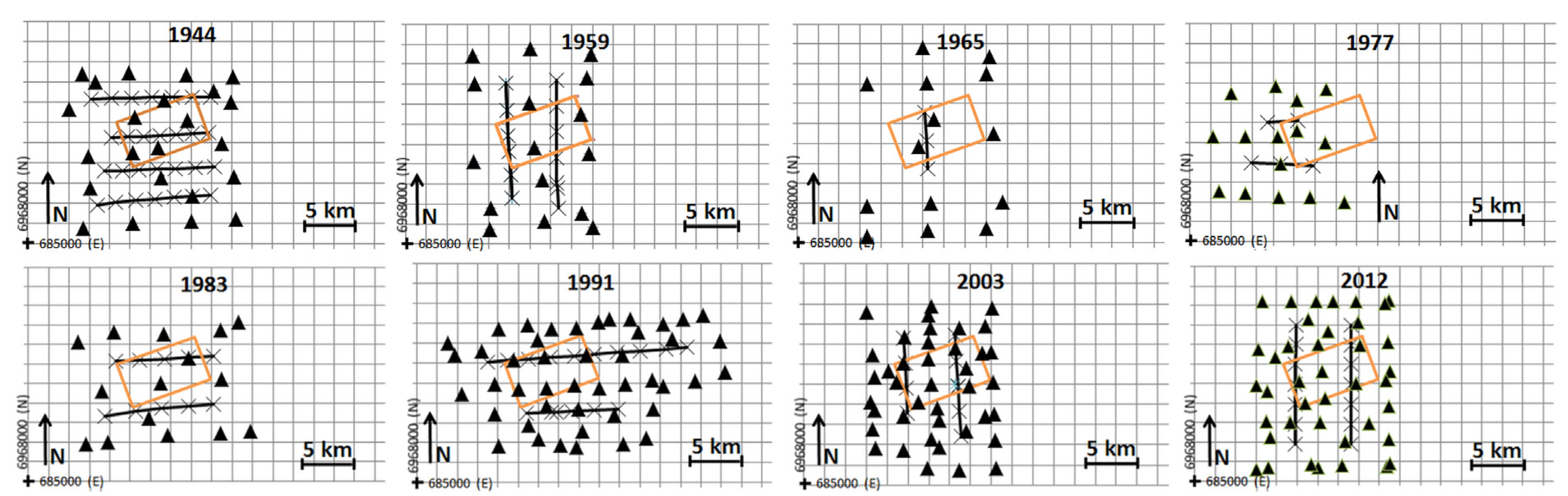
The final self-calibrating bundle block adjustments were calculated after the approximate exterior orientations were accurate enough. The images from different years were handled as separate blocks and individually tied to an open data set. Large number of automatic tie points (approximately 145 per image) was measured in each block. GCPs were measured interactively and the number of GCPs per block varied between 15 and 45 (Figure 2). For the GCPs, we tried to find unchanged object locations; these locations included capes and small bays along the shoreline, the edges of meadows, islets, detectable features in bogs, pools, rocks, crossroads, sike crossings, elevated dry spots in bogs, ditch and road crossings, creek bends, ditch overpasses and stunted bushes. The GCPs were visually observed using open data from the NLS; colour orthoimages and a 10 m elevation model were used. For weighting purposes, standard deviations were estimated at 2 m for the X, Y and Z coordinates of the GCPs and 0.5 pixels for image’s x and y coordinates for the tie points and GCPs.

Self-calibration was done for all of the image blocks. A well-known set of physical parameters with a principal point of best symmetry (PBS) (x_PBS, y_PBS) and three radial (k1, k2, k3) and two decentring terms (p1, p2) were set as the unknown parameters [44,45,46]. For the 1944 and 1959 blocks, eight interior orientation, bilinear coefficient correction parameters were also calculated–per camera for 1944 and per film type for 1959.

In most cases, there were two or more flight lines and the area of interest (ALS coverage area) was located between the flight lines (Figure 2). Data from 1965 have a lower spatial resolution than the other data sets and comprised only a single flight line. The 1977 data images did not completely cover the area of interest.

Figure 2. Flight lines and ground control points. The rectangular area (orange colour) shows the coverage of the ALS data.

Figure 2. Flight lines and ground control points. The rectangular area (orange colour) shows the coverage of the ALS data.

2.3.3. DSM Generation

For the generation of dense DSMs, the Next Generation Automatic Terrain Extraction (NGATE) of SOCET SET V5.6.0 was used [47]. We used a predefined matching strategy called “ngate_urban_noisy.strategy”, which is suitable for matching in an environment with large height differences, such as forest. We allowed three image pairs per point during matching. The matching strategy utilised image resolution pyramids with seven pyramid layers with a reduction factor of two between the layers. Final matching was carried out using the full resolution images. The most important parameter in this method is the correlation window size during the area-based matching phase, which was a constant 13 × 13 pixels in each pyramid layer. Surface models were created in grid format with a 1 m point interval. The NGATE software provides a figure of merit value (FOM) for each match indicating the quality of the matching. FOM values lower than 40 indicate different exceptional situations, and failed matching and values between 40 and 100 indicated successful correlations. When the FOM value was 40–100, the elevation value was based on the image matching; if the FOM value was lower, the height value was interpolated.

2.4. DSM Uncertainty Estimation

The uncertainty budget of the DSM measurement contains three major components: photogrammetric modelling error, object measurement error and surface modelling error [48]. The photogrammetric modelling error results from the uncertainty of the ray intersection, which is dependent upon the accuracy of the exterior orientation, interior orientation and intersection geometry. The object measurement error is highly dependent upon the target properties. For example, for symmetrical, well-defined targets, such as signalled points, the measurement error is part of the GSD. The expected measurement error of vague objects is much larger, for example 0.2 m–1 m for trees [49]. The surface modelling error is dependent upon the object’s topography and the point density, i.e., how well the discrete representation represents the real object’s 3D structure. For dense point cloud data, the first two uncertainty components are the most significant. In this investigation, our emphasis was on estimating the photogrammetric modelling error.

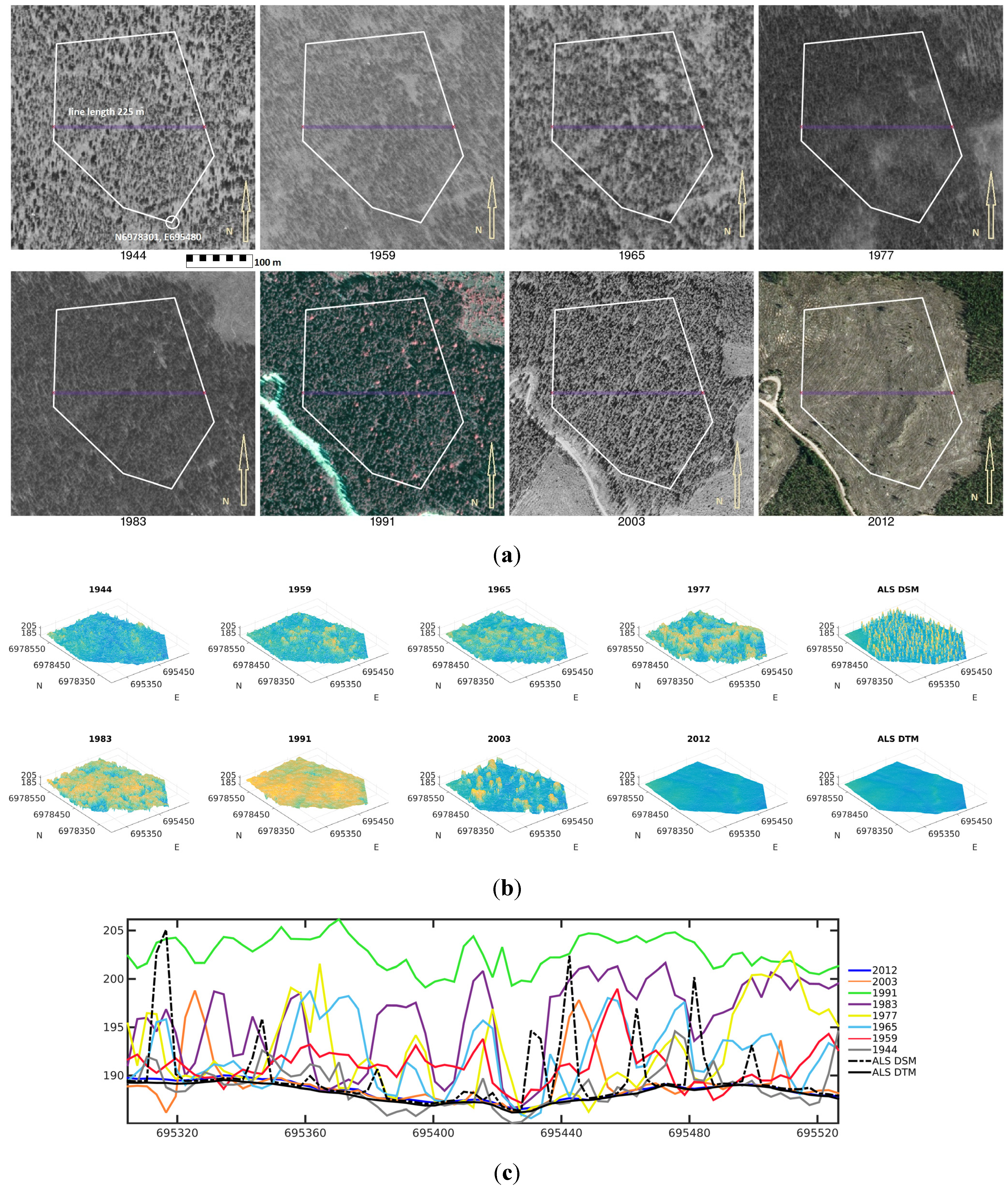
Evaluating the accuracy of the historical DSMs was a challenge due to the lack of stable reference targets as well as the great number of landscape changes during the 68 year period of time. The photogrammetric modelling error was evaluated at the locations with minimal vegetation coverage in order to provide good stability, and it was explicit in order to provide an object measurement error that was as low as possible. In the Palokangas study area, these kinds of locations were typically roads and treeless peatland areas. ALS was considered to be the ground truth. The ALS point cloud was processed into DSM and DTM grids with the same coordinates as the photogrammetric grids. Orthomosaics were created using the NLS open data 10 m elevation model.

A procedure was developed to use roads when estimating the photogrammetric modelling error. A road mask was created using road vectors from the Topographic Database. The existence of the roads throughout the timeline was ensured via a visual inspection of the 1944 orthophoto, and only the roads that were visible in it were used. A comparison of the orthophotos from different years and the road vectors revealed that in many places the road line had changed, even though the location was approximately the same. A road type classification was available in the Topographic Database and we performed the analysis separately for the different classes. Roads from four classes were present in the study area: Class (I) road width of 5–6.5 m; Class (II) road width of 3–4 m; Class (III) road width of less than 3 m; Class (IV) a drive path. The number of visible roads increased over time.

The accuracy assessment was done in test areas, TA = {ta₁, ta₂, … ta_n}, that were formed based on road vectors in the Topographic Database. All points with a planar distance of 2 m or less from the road vector were included in the test area, which consisted of each road segment visible in the orthoimage from 1944. Let $Z_{DSMy,ta}$ denote the photogrammetric points inside each test area, ta, from years = {1944, 1959, 1965, 1977, 1983, 1991, 2003, 2012}, and let y ∊ years and $Z_{DTM,ta}$ represent the respective points on the ALS-derived DTM. The photogrammetric DSM points include only points with a FOM figure ≥ 40. The road level absolute error, RE, from the ALS ground level in each point was computed using Equation (1):

$$R{E}_{y,ta}=\sqrt{{\left(Z_{DSMy,ta}-Z_{DTM,ta}\right)}^2}$$

(1)

The road points were filtered to remove vegetation points. Larger than threshold values for RE in Equations (2) and (3) were rejected. Equation (3) was used instead of Equation (2) if, after using Equation (2), the std of the remaining points was > Z_lim. If this was the case, we used Z_lim = 7 m in the equations.

$$R{E}_{y,ta}>std\left(R{E}_{y,ta}\right)\times 2$$

(2)

$$R{E}_{y,ta}>median(R{E}_{y,ta})$$

(3)

For the filtered points, the median RMSE (Root Mean Squared Error), MedRMSE, was computed for each road class, C, using Equation (4):

$$MedRMS{E}_{y,C}=median\left(\sqrt{\frac{{{\displaystyle \sum }}_{ta}{\left(Z_{DSMy,ta}-Z_{DTM,ta}\right)}^2}{n_{ta}}}\right)$$

(4)

The median was computed for all test areas that belonged to class C, and $n_{ta}$ was the number of points in area ta. There were three cases where Equation (3) was used. Two of them occurred at the same road segment in different years and two of them in the same year, 1991. MedRMSE_y,C was used as an estimate of the DSM height error.

In order to compare performance of different objects, test patches were also determined as polygons within the Topographic Database’s land cover polygons and 2012 orthoimage (Figure 1, Section 2.5). With a similar notation for points inside the test area, the RMSE statistics were computed for each class using FOM value-based point selection.

2.5. Change Evaluation

We used the Topographic Database’s polygons to select areas that have different land cover classes. We evaluated the change in the main land cover classes: “peatland without trees”, “peatland with trees” and “open forestland”. There were not enough samples from the other classes that could be included in the study (Figure 1). Test patches were drawn inside the original polygons to acquire samples that were comparable and to avoid edge effects. The original polygons had a complex shape, were of different sizes and had different outline length/area ratios. The selected test patches are not equal in size or complexity, but the diversity is considerably lower than in the original polygons. The variation in the DSM height within these areas was studied in order to find land cover types that have systematically low temporal variations in height. The “open forestland” class consists mainly of areas that were clear-cut at the time of the ALS acquisition. The ALS-derived DSM was not representative of the forested area, so we created additional test areas according to the 2012 orthoimage in order to have ALS statistics from a forested area (class “forest 2012”).

Changes in the canopy height during the timeline for the images in each class were assessed by computing a maximum change matrix and estimating growth from periods of consecutive increase in height. The maximum height change map was constructed on a pixel-wise basis, with $Z_{DSMy}$ denoting all points of the year, y. The maximum change is taken in time dimension for each location/pixel, as shown in Equation (5):

$$\max Change=\text{max}(\left\{Z_{DSMyn}-Z_{DSMy(n-1)},Z_{DSMy\left(n-1\right)}-Z_{DSMy\left(n-2\right)},\dots ,Z_{DSMy2}-Z_{DSMy1}\right\})$$

(5)

The estimate of the annual growth was computed first for each test patch using the test patch’s mean height (mh), Equation (6), where $n_{ta}$ was the number of points in area ta. For each test patch, the maximum mh was found and the timeline was stepped backwards from the time of the maximum (start). End of the decreasing trends (stop) was met if the next sample was not descending in height. Height and time differences between these samples were used to compute the yearly growth estimate, $y{g}_{ta}$, for the patch, Equation (7).

$$m{h}_{y,ta}= \frac{{{\displaystyle \sum }}^{\text{}}(Z_{DSMy,ta})}{n_{ta}}$$

(6)

$$y{g}_{ta}=\frac{(m{h}_{start,ta}-m{h}_{stop,ta})}{(year{s}_{start}-year{s}_{stop})}$$

(7)

The class growth estimates were computed as means of $y{g}_{ta\in class}$, which belong to each class.

3. Results

3.1. Quality of Georeferencing

3.1.1. Fiducial Transformations

The first task was to establish the fiducial transformation for the images in which the calibrated fiducial coordinates were not available (1944, 1959). We measured the dot-like fiducials of the image block collected in 1944 interactively. In total, we measured 112 fiducials (four fiducials in 28 images). We converted the pixel coordinate system into temporary image-wise, fiducial centroid-centred systems. For the new systems, we took into account slightly different scanner pixel sizes in perpendicular directions. The direction of the x-axis was chosen so that the two fiducials located approximately in the flying direction received equal y-values. Hence, the positive x-axis pointed right and the positive y-axis pointed up. Now, the side lengths from the opposite fiducials could be calculated (Figure 3). Eventually, we averaged artificial fiducial locations from the image-wise data and used them as replacements for the missing camera calibration values.

Figure 3. Image length in the x- (left) and y-direction (right) for the 1944 images.

Figure 3. Image length in the x- (left) and y-direction (right) for the 1944 images.

The 1944 image block consisted of four flying strips, each having seven images. The first flying strip had the greatest distortions (Figure 3). Curiously, by looking at the average values, the first and the third strip and, comparably, the second and the fourth strip had almost equal image lengths in the x-direction (that is, pointing in the flight direction as well as the film-roll direction). The first and the third strip were flown in an easterly direction and the second and the fourth strip in a westerly direction. One possible explanation might be the differences in the film flattening while the aircraft is flying in the opposite directions. We also detected a large degree of variation in the lengths between the opposite fiducials. Moreover, the average lengths in x-direction and y-direction were different; one possible explanation could be different stretching of film in two directions. For the 1959 image set, an artificial interior orientation was performed similarly to the 1944 case.

Residual statistics for the affine fiducial transformations (Table 3) show that the residuals of the images captured in 1944 were the largest; RMSEs were at the level of approximately 40 µm. The residuals were on low level (6–7 µm) for the image blocks since 1959.

Table 3. Quality statistics for the film’s imagery interior orientation: maximum, minimum and average RMSE of residuals. |MAX RES| = Maximum residual. Statistics for the interior orientation via the scanner were not available for image blocks captured in 1965 and 1977.

Year	MAX RMSE (µm)	MIN RMSE (µm)	AVE RMSE (µm)	|MAX RES| (Pixels)
1944	85.60	23.40	40.05	5.71
1959	11.20	2.50	5.94	0.75
1983	10.00	2.70	5.71	0.64
1991	8.10	5.40	7.03	0.80
2003	8.30	5.00	6.92	0.61

Table 3. Quality statistics for the film’s imagery interior orientation: maximum, minimum and average RMSE of residuals. |MAX RES| = Maximum residual. Statistics for the interior orientation via the scanner were not available for image blocks captured in 1965 and 1977.

Year	MAX RMSE (µm)	MIN RMSE (µm)	AVE RMSE (µm)	|MAX RES| (Pixels)
1944	85.60	23.40	40.05	5.71
1959	11.20	2.50	5.94	0.75
1983	10.00	2.70	5.71	0.64
1991	8.10	5.40	7.03	0.80
2003	8.30	5.00	6.92	0.61

3.1.2. Self-Calibrating Bundle Block Adjustments

The standard deviation estimates of the bundle block adjustment show the expected quality of the image blocks under ideal conditions when there exist only random errors. The RMSEs of the standard deviations in the positions of the perspective centres were 0.2–1.0 m in X0 and Y0 and 0.1–0.5 m in Z0. The RMSEs for the image rotations were 0.003–0.007° for v and f and 0.001–0.003° for k (Table 4). These values indicated a good level of accuracy for the image blocks.

Table 4. RMSEs of the point unknowns (X, Y and Z) (theoretical point determination error estimates) and the exterior orientation parameters (X0, Y0, Z0, v, f, k) based on the standard deviation estimates for the bundle block adjustment

Year	RMSE X (m)	RMSE Y (m)	RMSE Z (m)	RMSE X0 (m)	RMSE Y0 (m)	RMSE Z0 (m)	RMSE v (°)	RMSE f (°)	RMSE k (°)
1944	0.17	0.18	0.64	0.60	0.61	0.26	0.0053	0.0052	0.0015
1959	0.38	0.29	0.63	0.24	0.25	0.11	0.0028	0.0028	0.0014
1965	0.66	0.64	1.51	0.93	0.92	0.50	0.0045	0.0049	0.0022
1977	0.19	0.21	0.62	0.95	0.91	0.54	0.0069	0.0071	0.0029
1983	0.17	0.21	0.60	0.67	0.69	0.40	0.0053	0.0052	0.0020
1991	0.28	0.33	0.98	0.60	0.60	0.27	0.0047	0.0046	0.0015
2003	0.32	0.27	0.68	0.42	0.40	0.25	0.0038	0.0042	0.0019
2012	0.27	0.16	0.90	0.57	0.81	0.26	0.0059	0.0040	0.0016

Table 4. RMSEs of the point unknowns (X, Y and Z) (theoretical point determination error estimates) and the exterior orientation parameters (X0, Y0, Z0, v, f, k) based on the standard deviation estimates for the bundle block adjustment

Year	RMSE X (m)	RMSE Y (m)	RMSE Z (m)	RMSE X0 (m)	RMSE Y0 (m)	RMSE Z0 (m)	RMSE v (°)	RMSE f (°)	RMSE k (°)
1944	0.17	0.18	0.64	0.60	0.61	0.26	0.0053	0.0052	0.0015
1959	0.38	0.29	0.63	0.24	0.25	0.11	0.0028	0.0028	0.0014
1965	0.66	0.64	1.51	0.93	0.92	0.50	0.0045	0.0049	0.0022
1977	0.19	0.21	0.62	0.95	0.91	0.54	0.0069	0.0071	0.0029
1983	0.17	0.21	0.60	0.67	0.69	0.40	0.0053	0.0052	0.0020
1991	0.28	0.33	0.98	0.60	0.60	0.27	0.0047	0.0046	0.0015
2003	0.32	0.27	0.68	0.42	0.40	0.25	0.0038	0.0042	0.0019
2012	0.27	0.16	0.90	0.57	0.81	0.26	0.0059	0.0040	0.0016

The RMSEs of the standard deviations of the point unknowns (ground coordinates of the tie points) were mostly better than 0.3 m for the X and Y coordinates and 0.5–1.0 m for the Z coordinate (Table 4). The RMSEs were larger for the image block collected in 1965 due to the smaller image scale, approximately 0.7 m for X and Y and 1.5 m for Z. When scaling the RMSEs of X and Y using the imaging scale factor and the RMSE of Z using the flying height, the values from the different flying altitudes became more similar. In the image coordinates, these values were 5–10 µm in X and Y and 0.1‰–0.2‰ flying height in Z. The 1991 data set showed poorer relative standard deviation values for the point unknowns than the other data sets. One possible explanation for this is the slightly higher forward overlaps in the strip direction, which can cause lower B/H ratios as well as slightly lower side overlaps (Table 1). The RMSEs of the point unknowns provide the theoretical point determination error estimates of points with an image coordinate standard deviation of 0.5 pixels, and this is a quite feasible standard deviation estimate for the DSM points as well. It should be noticed that these are average values in the area of the entire block; the standard deviations are typically higher at block perimeters and lower at the centre parts of the block. The errors grow rapidly in the areas outside the GCP support and those areas should not be used in mapping.

We determined the improvements for the sensor parameters using self-calibrating bundle block adjustments (Table 5). The parameter changes were the greatest for the three oldest blocks. In many cases, the standard deviations were quite high, which indicated that the block geometry was not ideal for self-calibration.

Table 5. Improvements and standard deviations of the lens parameters determined by self-calibration.

Parameters	1944	1959	1965	1977	1983	1991	2003	2012
Parameter improvements
dxPBS (mm)	−2.6 × 10−2	−1.3 × 10−2	3.3 × 10−3	7.8 × 10−4	2.0 × 10−4	1.8 × 10−3	−4.9 × 10−4	6.5 × 10−4
dyPBS (mm)	5.2 × 10−2	1.3 × 10−1	−8.8 × 10−3	−5.1 × 10−4	1.8 × 10−3	−1.9 × 10−4	−1.3 × 10−4	1.1 × 10−3
dk1 (mm/mm3)	7.6 × 10−8	−1.0 × 10−6	5.2 × 10−9	−1.9 × 10−9	−7.0 × 10−9	−4.7 × 10−9	−2.2 × 10−9	1.7 × 10−8
dk2 (mm/mm5)	−5.7 × 10−12	1.3 × 10−10	6.9 × 10−14	−6.8 × 10−14	6.0 × 10−14	7.8 × 10−14	−1.4 × 10−14	−2.7 × 10−11
dk3 (mm/mm7)	1.6 × 10−16	−4.0 × 10−15	−7.5 × 10−19	1.5 × 10−18	3.1 × 10−19	6.8 × 10−19	4.7 × 10−20	3.4 × 10−15
dp1 (mm/mm2)	−9.4 × 10−8	3.1 × 10−7	−1.0 × 10−7	−1.1 × 10−8	−1.6 × 10−8	6.1 × 10−8	2.9 × 10−8	−4.9 × 10−8
dp2 (mm/mm2)	−3.9 × 10−8	−5.3 × 10−9	−9.0 × 10−9	6.0 × 10−8	4.0 × 10−8	2.5 × 10−8	2.0 × 10−9	−4.3 × 10−8
Standard deviations
σdxPBS (mm)	9.9 × 10−2	8.2 × 10−2	1.0 × 10−1	1.0 × 10−1	1.0 × 10−1	1.0 × 10−1	1.0 × 10−1	1.0 × 10−1
σdyPBS (mm)	9.9 × 10−2	7.9 × 10−2	1.0 × 10−1	1.0 × 10−1	1.0 × 10−1	1.0 × 10−1	1.0 × 10−1	1.0 × 10−1
σdk1 (mm/mm3)	1.4 × 10−8	2.6 × 10−8	6.7 × 10−9	5.2 × 10−9	3.0 × 10−9	1.6 × 10−9	3.2 × 10−9	5.4 × 10−8
σdk2 (mm/mm5)	2.3 × 10−12	4.9 × 10−12	2.6 × 10−14	3.5 × 10−14	1.5 × 10−14	1.4 × 10−14	1.7 × 10−14	3.1 × 10−11
σdk3 (mm/mm7)	1.2 × 10−16	2.8 × 10−16	4.3 × 10−19	6.6 × 10−19	2.0 × 10−19	2.1 × 10−19	2.9 × 10−19	5.4 × 10−15
σdp1 (mm/mm2)	1.4 × 10−8	2.0 × 10−8	3.9 × 10−8	3.3 × 10−8	1.9 × 10−8	1.7 × 10−8	2.9 × 10−8	6.1 × 10−8
σdp2 (mm/mm2)	1.3×10−8	2.2 × 10−8	2.9 × 10−8	2.5 × 10−8	1.6 × 10−8	1.5 × 10−8	2.4 × 10−8	5.1 × 10−8

Table 5. Improvements and standard deviations of the lens parameters determined by self-calibration.

Parameters	1944	1959	1965	1977	1983	1991	2003	2012
Parameter improvements
dxPBS (mm)	−2.6 × 10−2	−1.3 × 10−2	3.3 × 10−3	7.8 × 10−4	2.0 × 10−4	1.8 × 10−3	−4.9 × 10−4	6.5 × 10−4
dyPBS (mm)	5.2 × 10−2	1.3 × 10−1	−8.8 × 10−3	−5.1 × 10−4	1.8 × 10−3	−1.9 × 10−4	−1.3 × 10−4	1.1 × 10−3
dk1 (mm/mm3)	7.6 × 10−8	−1.0 × 10−6	5.2 × 10−9	−1.9 × 10−9	−7.0 × 10−9	−4.7 × 10−9	−2.2 × 10−9	1.7 × 10−8
dk2 (mm/mm5)	−5.7 × 10−12	1.3 × 10−10	6.9 × 10−14	−6.8 × 10−14	6.0 × 10−14	7.8 × 10−14	−1.4 × 10−14	−2.7 × 10−11
dk3 (mm/mm7)	1.6 × 10−16	−4.0 × 10−15	−7.5 × 10−19	1.5 × 10−18	3.1 × 10−19	6.8 × 10−19	4.7 × 10−20	3.4 × 10−15
dp1 (mm/mm2)	−9.4 × 10−8	3.1 × 10−7	−1.0 × 10−7	−1.1 × 10−8	−1.6 × 10−8	6.1 × 10−8	2.9 × 10−8	−4.9 × 10−8
dp2 (mm/mm2)	−3.9 × 10−8	−5.3 × 10−9	−9.0 × 10−9	6.0 × 10−8	4.0 × 10−8	2.5 × 10−8	2.0 × 10−9	−4.3 × 10−8
Standard deviations
σdxPBS (mm)	9.9 × 10−2	8.2 × 10−2	1.0 × 10−1	1.0 × 10−1	1.0 × 10−1	1.0 × 10−1	1.0 × 10−1	1.0 × 10−1
σdyPBS (mm)	9.9 × 10−2	7.9 × 10−2	1.0 × 10−1	1.0 × 10−1	1.0 × 10−1	1.0 × 10−1	1.0 × 10−1	1.0 × 10−1
σdk1 (mm/mm3)	1.4 × 10−8	2.6 × 10−8	6.7 × 10−9	5.2 × 10−9	3.0 × 10−9	1.6 × 10−9	3.2 × 10−9	5.4 × 10−8
σdk2 (mm/mm5)	2.3 × 10−12	4.9 × 10−12	2.6 × 10−14	3.5 × 10−14	1.5 × 10−14	1.4 × 10−14	1.7 × 10−14	3.1 × 10−11
σdk3 (mm/mm7)	1.2 × 10−16	2.8 × 10−16	4.3 × 10−19	6.6 × 10−19	2.0 × 10−19	2.1 × 10−19	2.9 × 10−19	5.4 × 10−15
σdp1 (mm/mm2)	1.4 × 10−8	2.0 × 10−8	3.9 × 10−8	3.3 × 10−8	1.9 × 10−8	1.7 × 10−8	2.9 × 10−8	6.1 × 10−8
σdp2 (mm/mm2)	1.3×10−8	2.2 × 10−8	2.9 × 10−8	2.5 × 10−8	1.6 × 10−8	1.5 × 10−8	2.4 × 10−8	5.1 × 10−8

Table 6. Quality statistics for the bundle block adjustments. RMS Image = The root mean squared value of the image residuals; RMSE X, RMSE Y and RMSE Z: the root mean squared value of the ground control point residuals.

Year	Number of GCPs	RMS Image (Pixels)	RMSE X (m)	RMSE Y (m)	RMSE Z (m)
1944	23	0.62	1.68	1.82	2.05
1959	25	0.95	1.60	1.57	1.63
1965	17	0.27	1.81	1.44	1.03
1977	15	0.30	0.96	0.73	0.63
1983	15	0.30	0.69	1.06	1.39
1991	45	0.24	0.58	0.55	0.56
2003	40	0.30	0.60	0.51	0.51
2012	40	0.14	0.55	0.58	0.54

Table 6. Quality statistics for the bundle block adjustments. RMS Image = The root mean squared value of the image residuals; RMSE X, RMSE Y and RMSE Z: the root mean squared value of the ground control point residuals.

Year	Number of GCPs	RMS Image (Pixels)	RMSE X (m)	RMSE Y (m)	RMSE Z (m)
1944	23	0.62	1.68	1.82	2.05
1959	25	0.95	1.60	1.57	1.63
1965	17	0.27	1.81	1.44	1.03
1977	15	0.30	0.96	0.73	0.63
1983	15	0.30	0.69	1.06	1.39
1991	45	0.24	0.58	0.55	0.56
2003	40	0.30	0.60	0.51	0.51
2012	40	0.14	0.55	0.58	0.54

We used the residuals in GCPs (Table 6) to estimate the 3D geometric accuracy of the blocks. The RMSEs were larger for the oldest blocks (1944, 1959, 1965). The RMSEs for individual coordinate axes were 1–2 m for the older blocks; for the blocks from the 1970s and 1980s, the RMSEs were 0.6–1.5 m, and for the blocks collected since 1990 the RMSEs were at the level of 0.6 m. These estimates were significantly more pessimistic, especially in the X and Y coordinate directions, than the theoretical point determination error estimates (Table 4), which is most likely due to the inaccuracy of the image and ground coordinates of the untargeted GCPs that also contribute to the total error.

3.2. Quality of DSMs

3.2.1. Overall DSM Quality Evaluation

We evaluated the success rate of image matching during DSM generation using the FOM values (Figure 4). In most cases, the FOM values were more than 40, which indicated that the image matching was successful; this means that the height points were matched points. Failures appeared mostly in the water areas and in some cases on the roads; in forests, some matching failures appeared due to occlusions. For the unsuccessful points, we interpolated the height values based on the surrounding points. During further processing, we only used the points demonstrating successful matching according to the FOM statistics. The FOM value provided by the NGATE is a relative measure, and it cannot be used to compare different image blocks.

Figure 4. FOM values for the 2012 (left) and the 1944 (right) image blocks.

Figure 4. FOM values for the 2012 (left) and the 1944 (right) image blocks.

The NGATE software provides relatively smooth DSMs in forest areas that do not penetrate to the forest floor. This can be observed in the DSM profiles in Figure 5 and Figure 6.

Profiles of a “peatland with trees” plot are shown in Figure 5. The forest growth and management operations can be observed in the profiles, e.g., logging after 1965 in the right part of the area and another logging operation after acquiring the ALS data.

Figure 5. Illustrations of a “peatland with trees” time series: (a) orthomosaic pieces with region of interest in white and profile location in light blue; (b) DSMs; (c) height profiles. Aerial images 1944–1965, photographed by Puolustusvoimat (PVTIEDL 214/2014). Aerial images 1977–2012 © NLS, 05/2013 and 07/2013. DTM in orthorectification and for the height of GCPs © NLS, Elevation Model 10 m, October 2013. Horizontal location for GCPs ©NLS, Colour Orthophoto, October 2013. Licences for the NLS data [36].

Figure 5. Illustrations of a “peatland with trees” time series: (a) orthomosaic pieces with region of interest in white and profile location in light blue; (b) DSMs; (c) height profiles. Aerial images 1944–1965, photographed by Puolustusvoimat (PVTIEDL 214/2014). Aerial images 1977–2012 © NLS, 05/2013 and 07/2013. DTM in orthorectification and for the height of GCPs © NLS, Elevation Model 10 m, October 2013. Horizontal location for GCPs ©NLS, Colour Orthophoto, October 2013. Licences for the NLS data [36].

Figure 6. Illustrations of an open forestland time series: (a) orthomosaic pieces with region of interest in white and profile location in light blue; (b) DSMs; (c) height profiles. Aerial images 1944–1965, photographed by Puolustusvoimat (PVTIEDL 214/2014). Aerial images 1977–2012 © NLS, May 2013 and July 2013. DTM in orthorectification and for the height of GCPs © NLS, Elevation Model 10 m, October 2013. Horizontal location for GCPs ©NLS, Colour Orthophoto, October 2013. Licences for the NLS data, [36].

Figure 6. Illustrations of an open forestland time series: (a) orthomosaic pieces with region of interest in white and profile location in light blue; (b) DSMs; (c) height profiles. Aerial images 1944–1965, photographed by Puolustusvoimat (PVTIEDL 214/2014). Aerial images 1977–2012 © NLS, May 2013 and July 2013. DTM in orthorectification and for the height of GCPs © NLS, Elevation Model 10 m, October 2013. Horizontal location for GCPs ©NLS, Colour Orthophoto, October 2013. Licences for the NLS data, [36].

As for examples of problems (Figure 6), visual inspection of the images indicated that within the plot, forest logging was not conducted before 2003; rather, it was conducted sometime between 2003 and 2012. The ALS-derived DSM shows that logging was carried out before 2008. In that area, however, the time series indicated that there were only a few trees in the 2003 data set and that the DSM mostly followed the forest floor. It is clear that the matching of the canopy surface failed for the 2003 data set.

Figure 7 shows an example of a DSM in a peatland without trees. There were great height variations in the early data sets (especially 1944). They were due to matching errors and an inaccurate imaging model. After 1965, the DSM was a smooth surface that followed the reference surface provided by the ALS quite well. It is possible that some part of the height variation in the 1944 data was due to the matching failures caused by the repetitive patterns on the surface of the peatland.

Figure 7. Illustrations of “peatland without trees” time series: (a) orthomosaic pieces with region of interest in white and profile location in light blue; (b) DSMs; (c) height profiles. Aerial images 1944–1965, photographed by Puolustusvoimat (PVTIEDL 214/2014). Aerial images 1983–2012 © NLS, May 2013 and July 2013. DTM in orthorectification and for the height of GCPs © NLS, Elevation Model 10 m, October 2013. Horizontal location for GCPs ©NLS, Colour Orthophoto, October 2013. Licences for the NLS data, [36].

Figure 7. Illustrations of “peatland without trees” time series: (a) orthomosaic pieces with region of interest in white and profile location in light blue; (b) DSMs; (c) height profiles. Aerial images 1944–1965, photographed by Puolustusvoimat (PVTIEDL 214/2014). Aerial images 1983–2012 © NLS, May 2013 and July 2013. DTM in orthorectification and for the height of GCPs © NLS, Elevation Model 10 m, October 2013. Horizontal location for GCPs ©NLS, Colour Orthophoto, October 2013. Licences for the NLS data, [36].

3.2.2. Determination of the Photogrammetric Modelling Error Using the Road Points

We used the road points to provide an empirical estimate of the photogrammetric modelling error (Table 7). For road classes I and II, the MedRMSE was 0.3–0.8 m for the data sets collected after 1970; for the older data sets the MedRMSE was 1–2 m (for 1965 only class I). The height error as fractions of the flying height was approximately 0.2‰–0.25‰ for the older blocks and 0.1‰ or better for the blocks collected after 1970. These results are consistent with the previous theoretical and empirical results (Section 3.1.2).

Table 7. RMSE statistics (MedRMSE, Min, Max) in metres between the photogrammetric DSM heights and ALS-DTM for road points; Points = the number of points is after filtering.

Road Type/Year RMSE (m) Median; Min; Max; Points	2012	2003	1991	1983	1977	1965	1959	1944	Total Number of Points
I: 6.5–5 m	0.44	0.46	0.65	0.49	0.78	1.59	0.93	1.33	19,781
	0.16	0.17	0.16	0.17	0.54	0.45	0.34	0.38
	4.02	4.77	4.33	4.25	1.61	3.29	1.86	2.72
	18,735	18,584	18,860	17,730	5669	18,800	19,062	19,149
II: 4–3 m	0.39	0.46	0.74	0.27	-	3.10	0.67	1.57	1587
	0.19	0.29	0.49	0.25	-	2.53	0.35	1.38
	0.43	0.90	0.83	0.34	-	4.12	0.78	2.03
	1392	1370	1327	1410	0	1386	1397	1405
III: <3 m	0.69	0.55	1.16	0.77	1.22	4.33	2.63	1.53	13,689
	0.11	0.20	0.11	0.22	0.35	0.89	0.18	0.54
	10.13	10.94	8.49	3.74	2.34	9.76	12.36	2.20
	12,774	12,891	12,344	12,971	4424	12,928	12,548	12,989
IV: drive path	1.20	0.61	8.44	5.21	2.09	2.54	1.18	1.77	3428
	0.20	0.39	0.52	0.19	-	1.76	0.51	1.03
	17.72	18.45	16.64	11.75	-	4.59	4.13	2.23
	3366	3352	3296	3266	456	3297	3252	3288

Table 7. RMSE statistics (MedRMSE, Min, Max) in metres between the photogrammetric DSM heights and ALS-DTM for road points; Points = the number of points is after filtering.

Road Type/Year RMSE (m) Median; Min; Max; Points	2012	2003	1991	1983	1977	1965	1959	1944	Total Number of Points
I: 6.5–5 m	0.44	0.46	0.65	0.49	0.78	1.59	0.93	1.33	19,781
	0.16	0.17	0.16	0.17	0.54	0.45	0.34	0.38
	4.02	4.77	4.33	4.25	1.61	3.29	1.86	2.72
	18,735	18,584	18,860	17,730	5669	18,800	19,062	19,149
II: 4–3 m	0.39	0.46	0.74	0.27	-	3.10	0.67	1.57	1587
	0.19	0.29	0.49	0.25	-	2.53	0.35	1.38
	0.43	0.90	0.83	0.34	-	4.12	0.78	2.03
	1392	1370	1327	1410	0	1386	1397	1405
III: <3 m	0.69	0.55	1.16	0.77	1.22	4.33	2.63	1.53	13,689
	0.11	0.20	0.11	0.22	0.35	0.89	0.18	0.54
	10.13	10.94	8.49	3.74	2.34	9.76	12.36	2.20
	12,774	12,891	12,344	12,971	4424	12,928	12,548	12,989
IV: drive path	1.20	0.61	8.44	5.21	2.09	2.54	1.18	1.77	3428
	0.20	0.39	0.52	0.19	-	1.76	0.51	1.03
	17.72	18.45	16.64	11.75	-	4.59	4.13	2.23
	3366	3352	3296	3266	456	3297	3252	3288

3.2.3. Assessment of Temporal Height Changes

We investigated the variability in the different land cover classes of “peatland without trees”, “peatland with trees”, and “forest 2012” using the MedRMSE statistics (Table 8). The results show that the variability in the “peatland without trees” class was on the level of 0.3–0.9 m for the data sets for the years 1983–2012, whereas for the DSMs calculated for the 1944–1977 image blocks the height variation was 0.6–2.2 m; this greater level of variation was due to the poorer accuracy of the DSMs. The “peatland without trees” class provided similar MedRMSE estimates as the road points especially for the widest road class (Table 7). This result supports our expectation that these objects remain unchanged in the time series; they are suitable candidates to be used as GCPs when automating the GCP measurement and they are also feasible for the assessment of the photogrammetric modelling error component of the heights in the DSM. The variations in the “peatland with trees” and “forest 2012” classes were much larger because of the trees. The variance was the largest in the “forest 2012” class. The values represent the photogrammetric modelling error and object measurement error as well as the height variations in the object.

Table 8. RMSE statistics (MedRMSE, Min, Max) in metres between the photogrammetric DSM heights and ALS-DTM for different land cover classes.

Land Cover Class/Year RMSE (m) Median; Min; Max	2012	2003	1991	1983	1977	1965	1959	1944	ALS
Peatland without trees	0.3	0.4	0.5	0.9	0.6	1.3	1.0	2.2	0.3
	0.2	0.3	0.2	0.3	0.3	0.9	0.4	0.9	0.1
	0.7	0.6	1.1	1.4	0.8	2.0	1.9	2.6	1.2
Peatland with trees	4.4	2.6	1.5	1.0	0.6	2.0	1.5	1.9	5.0
	0.2	0.2	0.2	0.3	0.4	0.6	0.5	0.8	0.3
	11.6	9.9	9.0	11.3	3.1	8.4	7.8	6.1	10.2
Open forestland	0.5	12.7	12.4	6.0	3.2	6.8	6.2	2.0	1.7
	0.2	0.4	5.7	1.2	2.4	3.0	1.8	1.1	0.4
	2.9	20.1	18.5	15.2	9.2	12.9	13.4	5.8	16.4
Forest 2012	11.2	6.9	7.6	3.0	0	2.6	6.1	2.1	9.9
	6.1	0.9	0.9	0.4	0	0.8	1.0	1.4	4.6
	16.0	13.9	12.1	15.4	4.7	16.0	15.9	10.4	13.2

Table 8. RMSE statistics (MedRMSE, Min, Max) in metres between the photogrammetric DSM heights and ALS-DTM for different land cover classes.

Land Cover Class/Year RMSE (m) Median; Min; Max	2012	2003	1991	1983	1977	1965	1959	1944	ALS
Peatland without trees	0.3	0.4	0.5	0.9	0.6	1.3	1.0	2.2	0.3
	0.2	0.3	0.2	0.3	0.3	0.9	0.4	0.9	0.1
	0.7	0.6	1.1	1.4	0.8	2.0	1.9	2.6	1.2
Peatland with trees	4.4	2.6	1.5	1.0	0.6	2.0	1.5	1.9	5.0
	0.2	0.2	0.2	0.3	0.4	0.6	0.5	0.8	0.3
	11.6	9.9	9.0	11.3	3.1	8.4	7.8	6.1	10.2
Open forestland	0.5	12.7	12.4	6.0	3.2	6.8	6.2	2.0	1.7
	0.2	0.4	5.7	1.2	2.4	3.0	1.8	1.1	0.4
	2.9	20.1	18.5	15.2	9.2	12.9	13.4	5.8	16.4
Forest 2012	11.2	6.9	7.6	3.0	0	2.6	6.1	2.1	9.9
	6.1	0.9	0.9	0.4	0	0.8	1.0	1.4	4.6
	16.0	13.9	12.1	15.4	4.7	16.0	15.9	10.4	13.2

Table 9. Estimate of the mean annual growth, yg (Equation (7)), with the standard deviation and mean growth period in years, with the last column showing the mean of the maximum absolute change between consecutive time samples for the land cover classes.

Land Cover Type	Mean Yearly Change (m)	Std of Yearly Change (m)	Time Period of Yearly Change	Mean Max Change (m)
Peatland without trees	0.07	0.06	28.7	2.2
Peatland with trees	0.10	0.08	29.7	4.0
Open forestland	0.28	0.12	32.7	13.6
Forest 2012	0.26	0.15	33.3	8.9

Table 9. Estimate of the mean annual growth, yg (Equation (7)), with the standard deviation and mean growth period in years, with the last column showing the mean of the maximum absolute change between consecutive time samples for the land cover classes.

Land Cover Type	Mean Yearly Change (m)	Std of Yearly Change (m)	Time Period of Yearly Change	Mean Max Change (m)
Peatland without trees	0.07	0.06	28.7	2.2
Peatland with trees	0.10	0.08	29.7	4.0
Open forestland	0.28	0.12	32.7	13.6
Forest 2012	0.26	0.15	33.3	8.9

We also evaluated the annual change (Equation (7)) in the different land cover classes (Table 9). The result was as expected. For the peatland classes, the annual average height change was 0.07–0.10 m with a standard deviation of 0.06–0.08 m; for the class “peatland without trees“ the change had a zero-mean over the entire period of time indicating no growth. For the “open forestland” and “forest 2012” classes, the change in mean annual height indicated a growth of 0.26–0.28 m with a standard deviation of 0.12–0.15 m. These values correspond well with the expected annual growth rate for a boreal forest.

4. Discussion

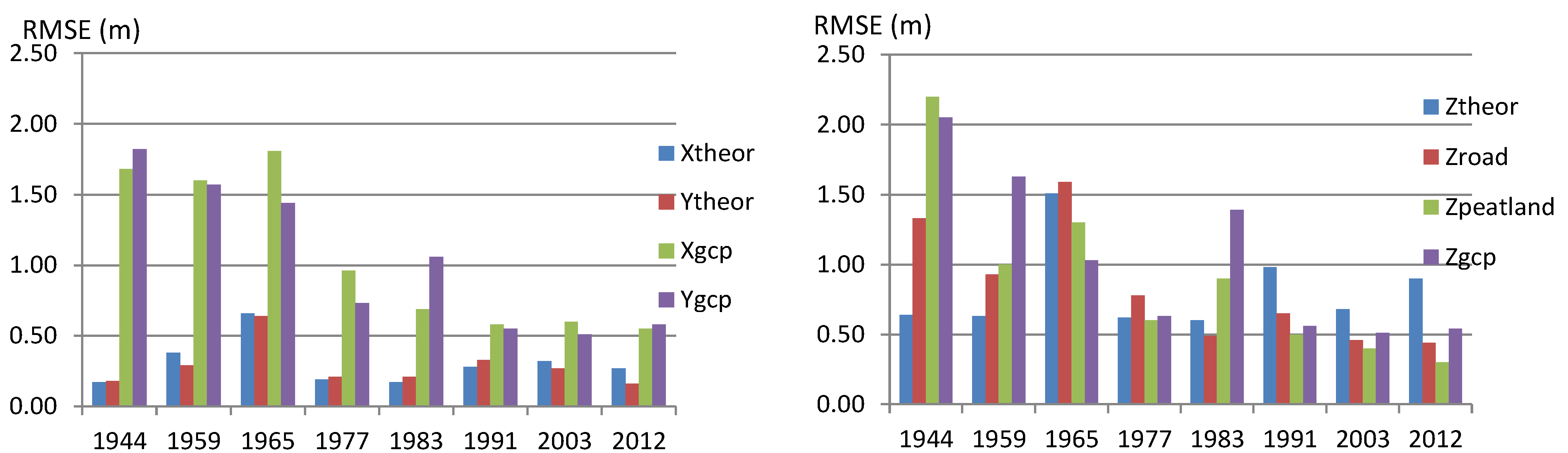
Our analysis provided various estimates of the performance of the photogrammetric point determination: theoretical point determination error estimates of the tie points, the residuals of GCPs and the median RMSEs (MedRMSEs) of DSMs on road and “peatland without trees” objects (Figure 8). These MedRMSE estimates could be considered as reliable and independent estimates of the photogrammetric modelling error component of the DSM height error, because the ALS data was not used in the photogrammetric processing and ALS height accuracy is at decimetre level in these objects. We had expected the estimates based on GCP residuals to be pessimistic because the reference coordinates were based on the topographic data sets (orthophotos and DTM) and their errors contributed to the calculated estimates. The theoretical estimates showed expected standard deviations of the points with a coordinate measurement error of 0.5 pixels, which can be a pessimistic value if the image materials and matching accuracy are high; this performance appeared for height error estimates of the new data sets (since the 1990s). On the other hand, theoretical estimates were optimistic for the oldest data sets (1944 and 1959) due to the poorer quality of the image materials. In further studies, the tuning of weights should be considered in order to obtain more realistic theoretical standard deviation estimates.

Figure 8. Theoretical and empirical accuracy estimates for horizontal (left) and height (right) coordinates. theor = theoretical point determination error estimates; road = MedRMSE for a road class of 5–6.5 m; peatland = MedRMSE of the “open peatland without trees” class; gcp = RMSE of the residuals of GCPs; X, Y and Z indicate estimates for the different coordinate axis.

Figure 8. Theoretical and empirical accuracy estimates for horizontal (left) and height (right) coordinates. theor = theoretical point determination error estimates; road = MedRMSE for a road class of 5–6.5 m; peatland = MedRMSE of the “open peatland without trees” class; gcp = RMSE of the residuals of GCPs; X, Y and Z indicate estimates for the different coordinate axis.

We considered three major components when modelling the height uncertainty budget of the photogrammetric DSM: photogrammetric modelling error, object measurement error and surface modelling error [48]. Our evaluations indicated that the photogrammetric modelling errors in well-defined targets were 0.3–0.9 m for the data sets collected since 1970; for the older data sets, they were 1–2 m. These values indicated a proportional height error of approximately 0.2‰–0.25‰ for the older blocks and 0.1‰ or better for the new blocks. These results are consistent with the expected level of accuracy for photogrammetric elevation measurements [49,50]. In this investigation, the GCPs were based on a national, open DTM and orthophotos. We assume that the level of accuracy could improve slightly as soon as new DTM and orthophotos based on ALS with a higher level of accuracy are available. However, these results provide the upper limit for the achievable accuracy for the materials used, because the blocks were well controlled with manually selected and measured GCPs.

When using a photogrammetric modelling error of 0.5 m and an object measurement error of 1 m for forested areas [49], the uncertainty propagation provides a height error estimate of 1.1 m for canopy heights; this is a quite feasible estimate for the image blocks collected after 1980. For the older image sets, a photogrammetric modelling error of 1.5 m provides an estimate of 1.8 m for canopy heights. This data quality is feasible for many forestry-related applications.

Possible explanations for the weaker geometric performance of the oldest data sets include the lower quality of the cameras and films as well as the aging and base of the film materials. For example, FMC-equipped cameras that eliminate a large part of the image blurring only became available in the 1980s. Also, film-flattening technology was improved during the film camera era and is unnecessary with digital cameras. Compensation for systematic image errors has been studied since World War II and has achieved a certain level of exactness in the self-calibrating bundle block adjustment. It must be understood that the quality of the images has followed the overall technological capabilities and fulfilled the requirements available at the time. With older imagery, constraining subsets of additional parameters according to the film being used and film development should be considered.

If the camera calibration data are unknown and the film material has been altered, the accuracy of the end product might be weak. In this study, we did not measure fiducials from all of the images from the film rolls. In high-accuracy production work, it would be worthwhile to automate the measurement process and to measure fiducials of all of the images on several film rolls originating from the same flight campaign and the same film material and processing to obtain a statistical foundation for the fiducial coordinates. Our interpretation of the results relating to the interior orientations of the blocks from 1944 and 1959 was that, although a great degree of roll-originated distortion was detected, it was uniform enough to be modelled in the case of the 1959 images. Possible causes for the weak interior orientations of the 1944 image block could be ageing variations in the film base material and film flattening problems during the flight. If drops form during the drying phase of film processing, local emulsion deformations up to ±20 µm can occur [49]. During the cellulose acetate film era, dimensional instability was a known problem in Finnish basic map production; stereo work had to be done with a glass plate base. Sometimes, the camera calibration data might be partly known or the necessary data may have been scattered across several documents; in our study, the camera used for the 1965 image block had the necessary camera information in three separately dated and partly conflicting documents. Our findings were similar to those from a study by Pérez et al. [51]; it is possible that the camera calibration data can be missing from historical aerial photographs and that film deformation can be considerable.

A practical observation about the data set used in this study was the fact that the image flights were not collected particularly for the purposes of this study. For two of the image blocks (1977 and 1991), the entire area of interest was not covered in stereo overlap. For two of the other image blocks (1959 and 2003), flying strips were not flown the same day. For one image block (2003), one flying strip consisted of images taken on two different dates. One image block (1991) had an extra image causing an almost 100% overlapping stereo model; the reason for this was a small cloud. We detected some scratches in the film emulsion. Scratches are common in film material due to film usage and they can cause errors in image matching. Depending on the software used for surface model generation, these kinds of details must be noticed in order to obtain the best-quality surface models.

The results show that, in general, the DSM matching was successful and provided consistent results. However, failures also occurred in some cases, for example with the block collected in 2003. Further evaluation of data suggested a few potential reasons. First of all, the data sets were from the early summer. One of the expectations is that the matching performance can be poorer in deciduous forests during the leaf-off period; in this case, this was not a likely reason, as the dominant tree species was Scots pine. The most likely reason for the failures in matching had to do with issues of multi-temporality. The block was collected in two parts, in June and July. The problematic test plot was located in the overlap area of these two data sets and had an overlap of approximately 100%. This might have caused two types of problems in image matching: first, the tie point matching can be inaccurate because of temporal differences, especially in shadows, causing poor orientation quality; second, the used photogrammetric software is sensitive to images having 100% overlap. We also created DSMs using images separately from June and July. The DSM was accurate when using the June data, while the July data were of poor quality. The most likely reason for the problems with the July data was inaccuracy in the exterior orientation due to the multi-temporal tie points.

Because of non-homogenous image data, some imperfections are inevitable. As there are several potential sources of failures, we suggest providing a comprehensive DSM-quality raster during the DSM generation phase. The software used in this investigation provided figure of merit statistics that can be used to characterise successful and unsuccessful areas. To better support the situation with multi-temporal data sets, it will be important to also include indicators of any problems with multi-temporal matching into the statistics. The indicator of the maximal view angle at each point should also be added to highlight areas where the occlusions might cause problems. Furthermore, the impact of the block geometry and the general point intersection quality should be propagated to the entire uncertainty budget; it is also necessary to provide more accurate estimates of matching accuracy based on the statistics provided by the matching software. Quality statistics for each elevation plot represent valuable information when analysing the data with automated methods; this will provide tools for users of these data sets to identify potential problem areas and to evaluate uncertainties of their analysis. We also discovered that by analysing the entire time series, it is possible to filter out gross errors. The results are also representative of the software used in this investigation. It is also possible that some other types of software will be less or more sensitive to shadows during multi-temporal matching. With respect to DSM creation errors, our findings are in line with those of Gruen [52], who noted the possibility of there being groups of gross errors in DSMs.

Image time series should be considered also from the perspective of the future. What could be done to enable the best possibilities for future applications of present-day image data? One recommended approach is to record all the relevant data, such as camera calibration, camera system calibration, exterior orientation, coordinate system data, image observations, ground observations and accuracy data, into a temporally traceable database. Map data and other location-expressing data (e.g., ALS data, forest compartment data, land parcel data) would be also important to preserve at certain time intervals.

We determined approximate orientations of two oldest data sets (1944, 1959) using structure from motion (SFM) based algorithms. The processing was successful and it can be expected that the SFM technologies are powerful also in the processing of historical data sets. We used VisualSFM software [42,43] that has been previously implemented to our processing line; in the further studies different methods should be evaluated because they have been shown to perform differently [53].

We studied the possibility of automating the selection of locations for ground control with as little change as possible with the help of the national Topographic Database’s land cover polygons and road vectors. The most promising non-changing areas in our test site belong to the “peatland without trees” class. Korpela [3] used hummocks and hollows in mire vegetation for multi-temporal tie points when the vegetation seemed unchanging, but also noted the elevation uncertainty due to possible changes in the water level. We considered that the use of roads would be more challenging, since in the study area the number of roads increased and the road lines changed during the study timeline; there can also be problems in matching due to homogeneous surfaces or due to difficulty to measure the road surface in deep shadows of forests. On the other hand, when using high-quality data, it is possible to identify the changes in road lines and restrict the registration to unchanged targets. It is also possible to use control points that only partially cover the time series interval. The roads provided a reasonably stable, non-changing target that reached all sides of the study area, and they thus constituted feasible reference data. The challenge is how to ensure that the locations marked using the reference ALS DSM and Topographic Database road vectors were also roads in the historical DSMs. The larger differences in the road levels between the ALS and photogrammetric DSMs in the early blocks (up until 1983) may be caused by the following issues: the study area is rural and distant, so probably the width of the roads was not the same in the early years of the time series and the cameras and imaging technology were not as developed as in the later years. Other possible unchanged targets in the Finnish countryside could be buildings, field corners and ditch crossings. When the unchanged positions have been located, the next step involves the automatic matching of multi-temporal materials. The classical method for doing this is image matching, but an even more robust approach is likely to be an approach based on matching the DSMs [54]. The automatic selection of suitable candidate locations also helps if the final measurement of GCPs is performed manually.

Our approach differed from that of Korpela [3] and Véga and St-Onge [4] in several constitutive matters. In the study by Korpela, tie points were manually measured and 47% of the tie points were multi-temporal; Véga and St-Onge used Förstner features and cross-correlation for non-multi-temporal tie point measurements and semiautomatic DSM-matching for GCPs. Our tie points were calculated automatically per vintage. In the image orientation step, we tied each year’s images separately to the newest NLS open data from 2012 by manually measuring horizontal locations from an orthophoto and the corresponding heights from an elevation model. The image scale range used by Korpela varied from 1:5 K–1:30 K, while ours consisted of substantially smaller scales ranging from 1:30 K–1:60 K (film images). The image scale used in the study by Véga and St-Onge varied even in a tighter range from 1:12 K–1:15.84 K. Korpela had calibration certificates for all of the images, whereas in our study the two earliest vintages were supplied only with accurate focal lengths. Véga and St-Onge had one image vintage, for which only a nominal focal length was known. Korpela could use accurate targeted GCPs, while we utilised open data from the NLS for georeferencing. We used self-calibration in the bundle block adjustment, but Korpela did not. We did not use direct georeferencing data for the bundle block adjustment; Korpela, however, used such data for some tests. Finally, we included a comprehensive photogrammetric uncertainty propagation analysis in our study.

In order to further automate the georeferencing and analysis process of photogrammetric aerial image archives, we suggest that the following developments would need attention: automating the measurement process for fiducial transformation when the camera calibration information is not available, developing automatic methods to match multitemporal data sets in the stable locations, and generation of a DSM quality statistic layer that takes into account all relevant uncertainty factors of multitemporal DSMs. This investigation considered in particular the boreal forest biome; also, automated processing in different scenes is of importance and similar methods for identifying stable objects are also feasible in these cases.

We expect that the 3D environmental model time series information from forests covering entire countries would be valuable information in many applications that depend on information about forest dynamics. For example, forest growth and yield research, site index determination, disturbance dynamics research and many scenery-level spatial analyses could utilise time series information derived from image archives. Historical time series can provide the means for predicting future landscape changes, the timing of forest management practices or risk assessment and forest health management. Our results show that the automation aspects of generating these time series are promising when utilising modern photogrammetric tools.

5. Conclusions

We studied the aspects and possibilities for georeferencing small-scale, aerial image time series in a Finnish boreal forest area. Furthermore, we also studied the potential of generating dense 3D digital surface models via image matching using these data sets.

Our accuracy results conformed to our theoretical and practical expectations. We demonstrated that with historical (i.e., before 1960) imagery, it is difficult to achieve an accuracy level common to modern large-format aerial cameras. However, with a thorough self-calibration during the bundle block adjustment and by statistically simulating the missing camera calibration, it is possible to achieve a passable level of accuracy for many applications.

Our major objective was to contribute to automating the georeferencing process by investigating the possibility of finding stable objects in forested scenes that could be used as safe areas for tying old images to more recent images. Our results show that it is possible to find ground locations with little object-level change. We found that road classes I (width 5.0–6.5 m) and II (width 3.0–4.0 m) and “peatland without trees”, classifications provided by the Topographic Database of the National Land Survey of Finland, were good candidate areas for ground control. We also developed statistical methods for analysing the stability of the object. However, the maximum RMSE values related to these classes suggest that prior acceptance of candidate points, statistical testing of their quality should be done. In further investigations, the feasibility of the stable areas in automated or semiautomatic georeferencing should be evaluated.

In general, the generation of digital surface models (DSMs) based on photogrammetric image archives was highly successful. We also contributed to an uncertainty analysis of the DSM generation of photogrammetric aerial image archives. Our results also highlight some potential challenges in the process; our suggestion is to develop a comprehensive, high-quality statistical data layer for the DSM that can be used when analysing the data set.

Our results indicated that by using modern photogrammetric techniques, it is possible to reconstruct countrywide 3D environmental model time series with DSMs and orthophotos in a highly automated way. The small-scale photogrammetric archives cover many countries with a feasible temporal resolution. These time series can be useful in many applications, such as for measuring forest growth or landscape change.