1. Introduction
Remote sensing of phytoplankton abundance and distribution in coastal waters has relied on algorithms to estimate Chlorophyll
a (Chl
a), a pigment responsible for the conversion of solar energy for photosynthesis found in all photosynthesizing life forms [
1]. While there are accessory pigments such as Chlorophyll
b and Carotenoids, they have a considerably smaller impact in multi-spectral remote sensing [
2]. Chl
a preferentially absorbs energy in the blue and red wavelengths [
3,
4], which results in a relatively high reflectance in the green wavelength [
5]. Chl
a also fluoresces in the Near InfraRed (NIR) near 700 nm during photosynthesis [
6,
7].
Most of the existing satellite data products and algorithms focus on the blue and green spectra, which are more suited for the less complicated open ocean [
8]. However, remote sensing of Chl
a in Case 2 coastal surface water is more complicated compared to open ocean remote sensing because of several factors: absorption by Colored Dissolved Organic Matter (CDOM) [
9]; turbidity from non-organic and organic total suspended solids (TSS) [
10]; backscattering from shallow benthic vegetation such as submerged aquatic vegetation (SAV) [
11]; and benthic substrates that create significant noise in upwelling energy [
1,
12]. CDOM strongly absorbs in the blue part of the visible spectrum [
9,
13]. TSS strongly reflect in the red spectrum and induce backscattering in the blue spectrum [
14,
15]. Incident light may be able to reach the bottom and the reflection can be included in the composite upwelling spectral profile from the water surface if the water clarity is high and water depth is shallow [
16]. SAV, as with any other vascular, photosynthetic plants, absorbs Photosynthetically Active Radiation (PAR), reflects Near InfraRed (NIR), and therefore further alters the reflectance of the water [
17,
18]. The blue and green spectra can be impacted by Case 2 waters due to higher amounts of CDOM; and Chl
a can be examined with fewer complications through examining the red spectrum.
The MEdium Resolution Imaging Spectrometer (MERIS) package, aboard the European Space Agency (ESA) Environmental Satellite (ENVISAT), launched in March 2002 and provided a solution for these confounding factors of coastal waters, until the end of its mission in April 2012. MERIS had an ideal spectral resolution for measuring Chl
a in Case 2 waters, having 15 spectral bands from 390 to 1040 nm. MERIS data have spatial resolutions of 1.2 km for “Reduced Resolution (RR)” and 300 m for “Full Resolution (FR)” [
19]. RR is an average of 16 FR pixels and is made available more rapidly than FR [
20].
Gower
et al. [
7] built the first MERIS based algorithm for Chl
a, the Maximum Chlorophyll
a Index (MCI), which was able to model and track changes in Chl
a concentrations between 0.1 mg∙m
−3 and 19 mg∙m
−3. This approach uses bands centered at 681, 708 and 753 nm, as these longer wavelength bands are minimally affected by CDOM. In addition, the effects from TSS and water are speculated to be similar in red and NIR wavelengths [
21]. The most notable aspect of the MCI is the use of the 708 nm band which is centered over the Chl
a fluorescence. Gower
et al. [
8] found that while MERIS FR provided the best detail, the RR, when filtered to exclude land, was able to reduce noise generally at the expense of losing the ability to track small (<300 m) blooms. Atmospheric correction resulted in less accurate reports as most atmospheric correction methods were not designed with the Chl
a fluorescence peak in mind and subsequently overcorrected the red and NIR spectrums in areas of high Chl
a concentrations [
8]. Additionally, this algorithm is cautioned to be used as qualitative and was discouraged from use for estimating concentrations of Chl
a [
22]. As a result of the MCI, several Chl
a algorithms have been developed that utilize the MERIS 708 nm bands in an effort to estimate Chl
a concentrations utilizing FR reflectance data.
Dall’Olmo and Gitelson [
23] developed a three-band approach using bands 665, 708 and 753 nm. They chose 665 nm because 681 nm was believed to be influenced by the fluorescence of Chl
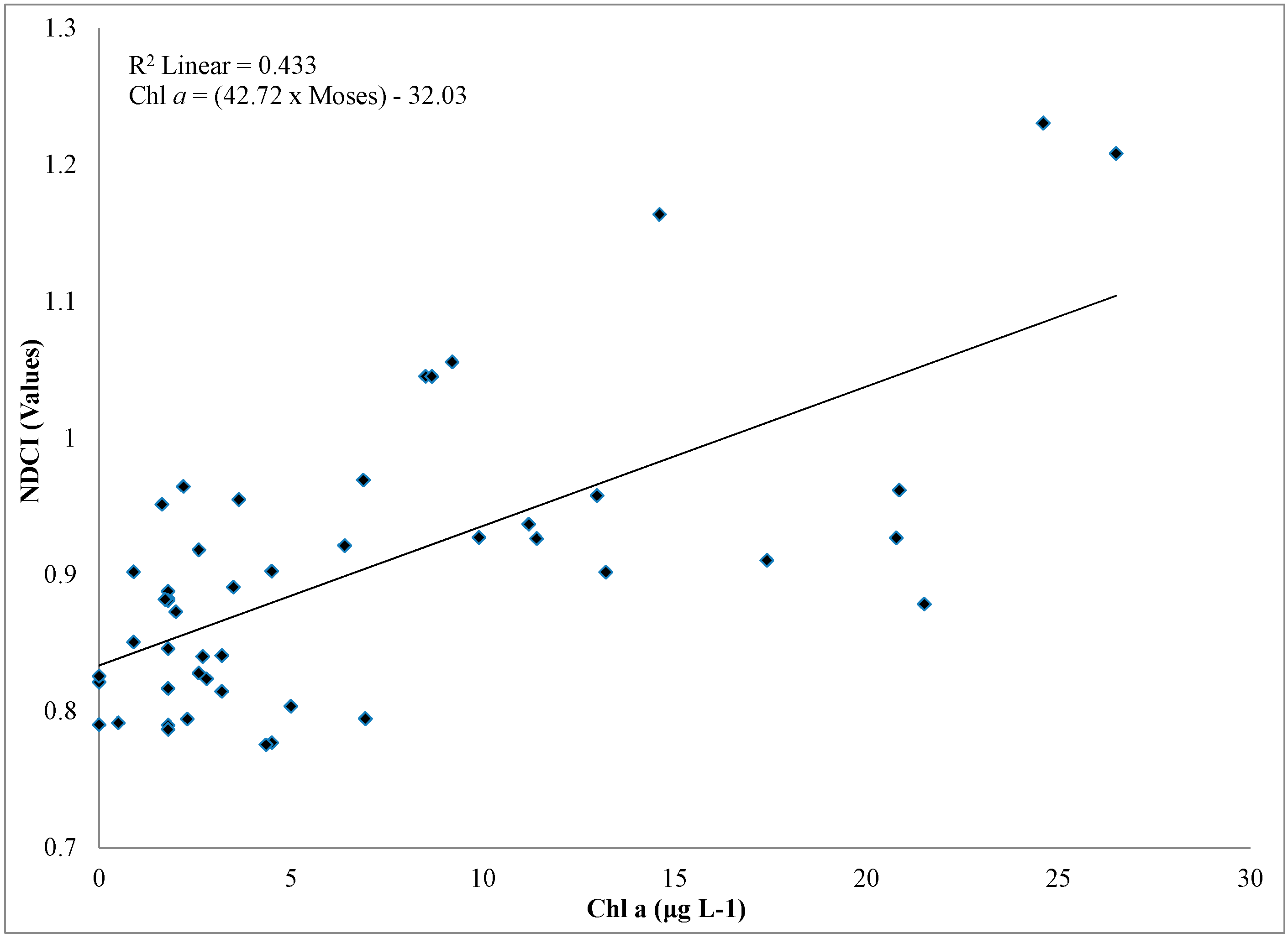
a. Their primary assumption with this model assumes that TSS affects all three bands equally. Moses
et al. [
24,
25] (Referred to as Moses in this paper) proposed returning to a two band ratio between 665 and 708 nm, due to the high rates of variability in three spectral points models. Mishra and Mishra [
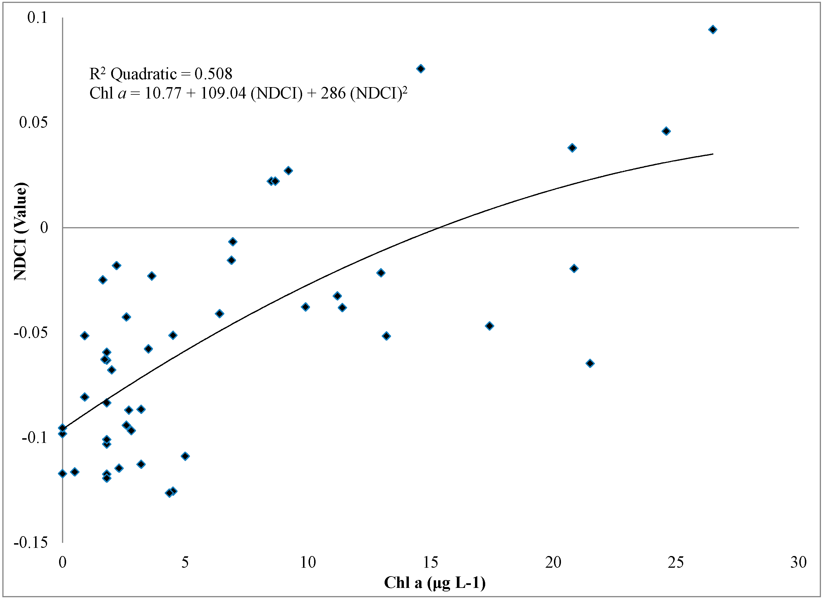
21] built the two band Normalized Difference Chlorophyll Index (NDCI) in an effort to improve models proposed by Moses
et al. [
25]. The NDCI uses 665 and 708 nm and operates similarly to the Normalized Difference Vegetative Index (NDVI) binding higher and lower index values between −1 and 1 and reducing seasonal variability and sun angle influences. A comparison of the NDCI effectiveness in Case 2 waters of the Chesapeake and Delaware Bays found NDCI was the most effective model, followed by Moses
et al. [
25] and then by Dall’Olmo and Gitelson [
23] (
Table 1). In a further effort to test the effectiveness of these algorithms for estuarine algal bloom mapping, we chose Moses
et al. [
25] and NDCI [
21] to calibrate and validate Chl
a in the Indian River Lagoon (IRL), FL a shallow estuary in which severe algal blooms have occurred in recent years.
Table 1.
Comparison of MERIS Chl
a estimation algorithms (Adapted from Mishra and Mishra [
21]). Dall’Olmo and Gitelson [
23] studied the Chesapeake Bay, USA; Moses
et al. [
24] studied the Sea of Azov; Mishra [
21] studied Chesapeake, Delaware, and Mobile Bays and the Mississippi Delta, USA.
Table 1.
Comparison of MERIS Chl a estimation algorithms (Adapted from Mishra and Mishra [21]). Dall’Olmo and Gitelson [23] studied the Chesapeake Bay, USA; Moses et al. [24] studied the Sea of Azov; Mishra [21] studied Chesapeake, Delaware, and Mobile Bays and the Mississippi Delta, USA.
| Method | Algorithm | R2 | RMSE (mg∙m−3) |
|---|
| Dall’Olmo and Gitelson [24] | | 0.43 | 3.09 |
| Moses et al., 2009 [25] | | 0.59 | 2.57 |
| Mishra 2011 [22] | | 0.72 | 2.15 |
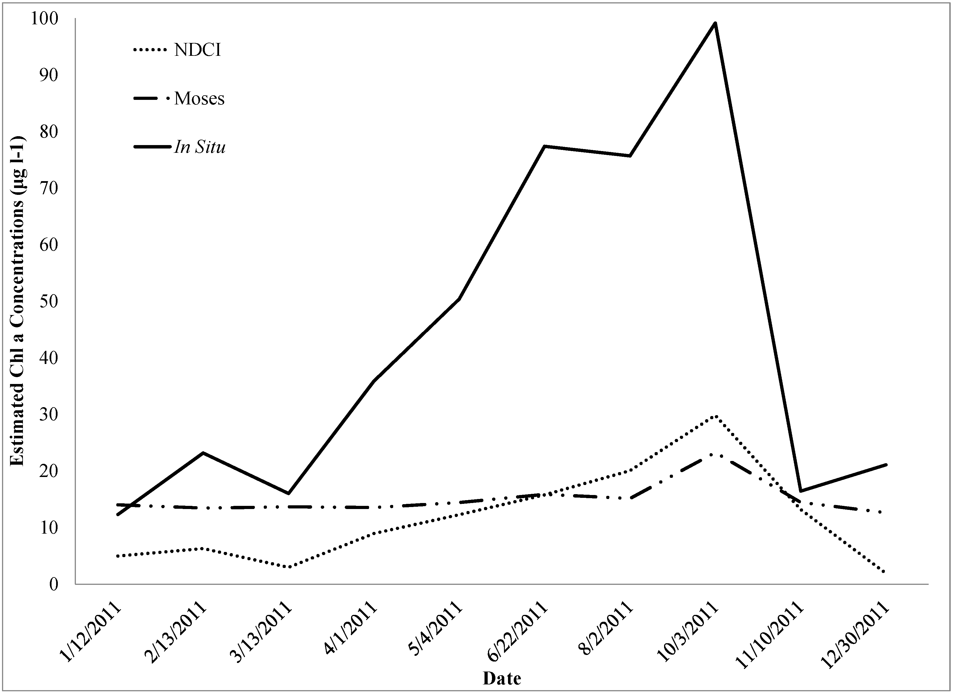
Starting in the spring of 2011, an unprecedented algal bloom occurred in Indian River Lagoon (IRL), FL, which lasted for seven months throughout the IRL system (SJRWMD 2012). During the blooms, the mean Chl
a was eight times the historical mean concentration (>50 µg∙L
−1 in most segments), which reduced light penetration through the water column and subsequently caused decreases in the density and distributions of SAV by up to 90% in some parts of the IRL [
26].
The St. Johns River Water Management District (SJRWMD), the state regulatory body for the IRL, has been monitoring water quality monthly at 56 sites in the IRL since 1996 to support total maximum daily load (TMDL) development and general ecosystem health analysis. Thirty four of these sites are located on the IRL and another 22 on the tributaries to the IRL. TMDL is a pollution reduction and regulatory method used in an effort to identify the maximum amount of nutrients, metals, and organic compounds a water body can receive while still meeting water quality standards [
27]. At “the historically normal conditions,” the IRL has an average Chl
a concentration range from 6.2 to 16.4 µg∙L
−1 [
26], with seasonal algal blooms at Chl
a levels reaching 25 µg∙L
−1. The long-term field water quality monitoring data at the multiple sites, however, were not sufficient to show spatially continuous information because the surface water area of the IRL is 750 km
2, meaning each monthly sampling site is used to assess an area of roughly 18 km
2 [
27]. Without spatially continuous visualization it was difficult to determine the spatial pattern of the bloom initiation, movement, and diminishment through the IRL.
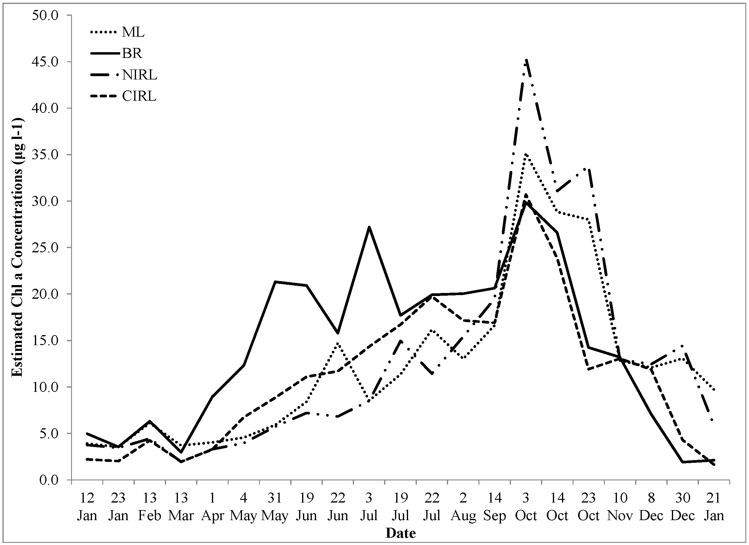
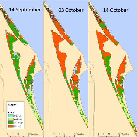
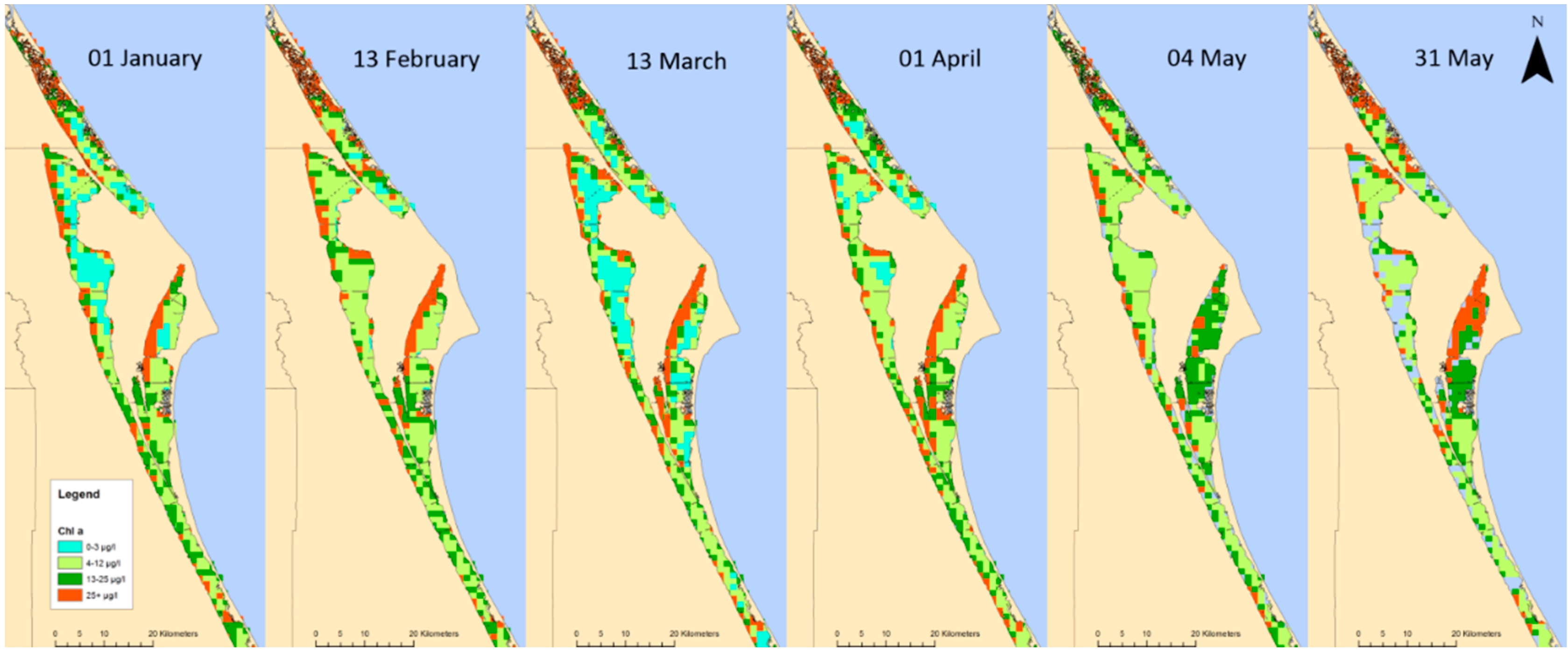
This study was conducted to visually analyze the 2011 algal bloom (SJRWMD 2012) event that occurred in the IRL system at a landscape scale utilizing MERIS satellite-based Chl a algorithms in order to provide additional information such as the bloom initiation, its progress and spatial expansion, and patterns of collapse. The three specific objectives were to (1) evaluate the NDCI and Moses using MERIS RR to determine the accuracy of the algorithms in estimation of Chl a in IRL, (2) map the 2011 algal bloom by using the algorithm that suggests to be most effective, and (3) provide spatially continuous visual analysis of the 2011 algal bloom to compare with in-situ water quality measurements.


