Article

Evaluation of Sampling Methods for Validation of Remotely Sensed Fractional Vegetation Cover

1
The State Key Laboratory of Remote Sensing Science, Beijing Key Laboratory for Remote Sensing of Environment and Digital Cities, School of Geography, Beijing Normal University, Beijing 100875, China
2
The State Key Laboratory of Resources and Environmental Information System, Institute of Geographic Sciences and Natural Resources Research, CAS, A11, Datun road, Beijing 100101 China
3
Jiangsu Center for Collaborative Innovation in Geographical Information Resource Development and Application, Nanjing 210023, China
*
Author to whom correspondence should be addressed.
Remote Sens. 2015, 7(12), 16164-16182; https://doi.org/10.3390/rs71215817
Submission received: 22 July 2015 / Revised: 11 November 2015 / Accepted: 19 November 2015 / Published: 2 December 2015

Abstract

:
Validation over heterogeneous areas is critical to ensuring the quality of remote sensing products. This paper focuses on the sampling methods used to validate the coarse-resolution fractional vegetation cover (FVC) product in the Heihe River Basin, where the patterns of spatial variations in and between land cover types vary significantly in the different growth stages of vegetation. A sampling method, called the mean of surface with non-homogeneity (MSN) method, and three other sampling methods are examined with real-world data obtained in 2012. A series of 15-m-resolution fractional vegetation cover reference maps were generated using the regressions of field-measured and satellite data. The sampling methods were tested using the 15-m-resolution normalized difference vegetation index (NDVI) and land cover maps over a complete period of vegetation growth. Two scenes were selected to represent the situations in which sampling locations were sparsely and densely distributed. The results show that the FVCs estimated using the MSN method have errors of approximately less than 0.03 in the two selected scenes. The validation accuracy of the sampling methods varies with variations in the stratified non-homogeneity in the different growing stages of the vegetation. The MSN method, which considers both heterogeneity and autocorrelations between strata, is recommended for use in the determination of samplings prior to the design of an experimental campaign. In addition, the slight scaling bias caused by the non-linear relationship between NDVI and FVC samples is discussed. The positive or negative trend of the biases predicted using a Taylor expansion is found to be consistent with that of the real biases.

Graphical Abstract

1. Introduction

Validation is necessary to ensuring the quality of a remote sensing product. Every product must pass a validation process prior to being provided to application disciplines [1,2]. The validation is often performed in representative regions by testing the remote sensing product in the same or similar place and time. The in situ data measured in the validation process generally represent a certain spatial scale, depending on the scale of the experimental plot and the heterogeneity. Compared to ground-based measurements, the spatial resolution of remote sensing products ranges from less than one meter to tens of kilometers. If the research attempts to monitor global change, coarse-resolution data must be used to provide sufficient revisit frequencies and temporal resolution [3]. However, qualifying the remote sensing data with data measured from a single ground plot is generally insufficient, especially on a heterogeneous land surface. More samples should be obtained to determine the value of a remote sensing pixel. Specifically, the information of points (samples) should be used to represent the information of a surface. Thus, selecting samples represents one of the most important problems in remote sensing product validation. A good sampling method can improve the accuracy of the estimation with fewer samples, whereas a poor sampling method increase costs and is of poor accuracy.
Sampling method and strategies have been applied in many large campaigns, e.g., the Boreal Ecosystem Atmosphere Study (BOREAS), the Validation of Land European Remote Sensing Instruments (VALERI) [4], the BigFoot project (for MODIS terrestrial product) [5] and the Southern African Regional Science Initiative (SAFARI2000) [6], to validate biophysical parameters [7]. In China, several comprehensive experiments were conducted in Heihe, Shunyi and Huailai [8]. A newly developed experiment, named Heihe Watershed Allied Telemetry Experimental Research (HiWATER), was implemented in the Heihe River Basin of China in 2012 to improve the ability to observe a hydrological process in an arid and semi-arid region [9]. Fractional vegetation cover (FVC), as a parameter to be obtained in this experiment [10], is an important element of climate models and significantly influences analyses and evaluations of an ecological environment. Generally, the validation of coarse-resolution satellite products of the FVC is performed based on a field campaign or FVC data from higher resolution satellites [11,12,13,14].
Sampling methods, such as simple random sampling, systematic sampling and stratified sampling, have been applied to the validation of remote sensing products [6,8] and other applications [15]. The advantage of these classical sampling methods is that they require minimal a priori information about the population and are easy to use [16,17]. Thus, they are commonly applied in different domains, including both spatial and non-spatial data analysis. However, such sampling methods commonly assume that samples are independent from each other, which is not the case in spatial sampling. According to Tobler’s law of geography, near objects are usually more correlated than distant ones [18]. Spatial sampling methods should consider the autocorrelations between geographically distributed objects, which can decrease the number of samples and improve sampling accuracy [19,20,21]. In practice, an optimization algorithm can be used to determine both the sample number and spatial position of the sample based on the relationship between spatial distance and autocorrelation [22,23,24,25]. Ordinary-kriging-based spatial sampling, as a typical method that considers spatial autocorrelation, has been applied in many studies, including for the calculation of vegetation cover, soil mapping, and meteorological network design [26,27,28,29,30]. Recent remote sensing field campaigns, such as VALERI [4], the European Space Agency’s (ESA) SENtinel-2 and FLuorescence Experiment (SEN2FLEX) [31] and HiWATER [32,33], have carefully considered spatial covariance in the sampling methods.
This paper focuses on the accuracy assessment and comparison of the sampling methods applied in FVC measurements. The tests are designed as realistically as possible to represent the situations in field campaigns. We first propose a framework to produce reference data. FVC maps are generated using Advanced Spaceborne Thermal Emission and Reflection Radiometer (ASTER) radiance images and the ground measurements of FVC. The ASTER-derived FVC is designated as the reference data. A spatial sampling method called mean of surface with non-homogeneity (MSN) [34] is then implemented in our designed scenes with the Normalized Difference Vegetation Index (NDVI) of ASTER and the land cover map. Three additional sampling methods, namely, simple random sampling, stratified random sampling and ordinary block kriging sampling (hereafter referred to as stratified sampling and ordinary kriging sampling, respectively), are also implemented for comparison purposes. This study attempts to compare the sampling methods on determining the samples for FVC product validation at a coarse scale from the perspective of expecting temporal as well as spatial variation.

2. Generation of Reference Data

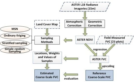
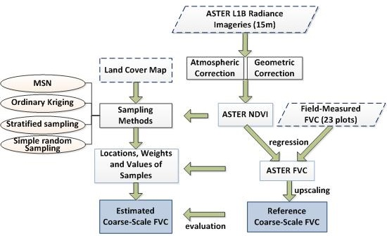
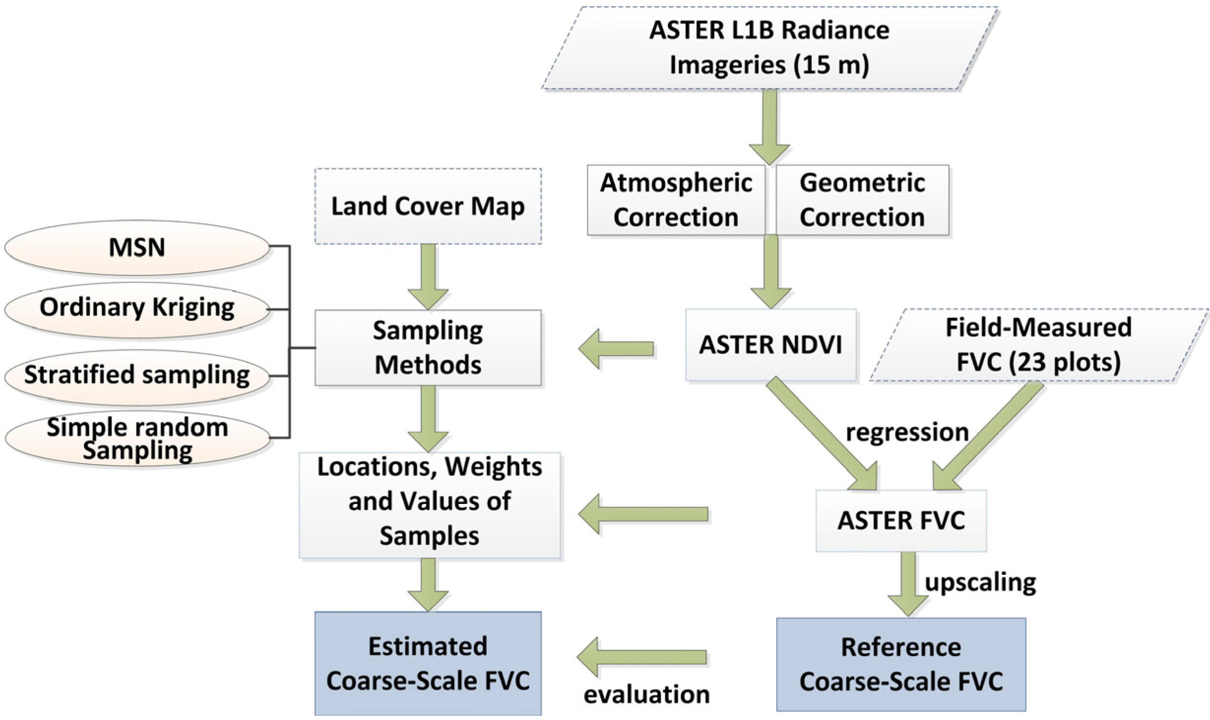
2.1. Framework of Reference Data Generation

In this study, the reference values of the FVC of coarse-resolution pixels (1 km), which were estimated from the 15-m-resolution images and field measurements, are introduced in the tests. The resolutions of reference FVC correspond to the spatial resolutions of typical coarse-resolution sensors [3] such as the Advanced Very High Resolution Radiometer (AVHRR), the Moderate Resolution Imaging Spectroradiometer (MODIS) and the Visible/Infrared Imager/Radiometer Suite (VIIRS) instrument. The sampling methods, through which locations and weights of samples were selected, could also generate FVC estimates at a coarse scale. Figure 1 shows a framework for generating the reference data of FVC and a comparison with the FVC estimated using the sampling methods. The accuracy of the estimated FVC at the coarse scale indicates whether a method is good.
Figure 1. Flowchart of generating reference fractional vegetation cover (FVC) at a coarse scale and a comparison with the estimated FVC.
Remotesensing 07 15817 g001
We used the ground measurement data and ASTER L1B radiance to generate the FVC data. The ASTER radiance data were first preprocessed with atmospheric corrections, thereby forming NDVI data. All the ASTER NDVI data were then spatially matched to the study region. The in situ FVC and ASTER NDVI data in the experimental region were regressed to obtain the reference FVC at a resolution of 15 m. The data from five crop growth states, representing the growing, saturation, and weathering periods of corn, were selected to validate the different sampling methods. The reference values, which were aggregated on a coarse scale by calculating the arithmetic mean, served as baselines in the comparison of the various sampling methods.

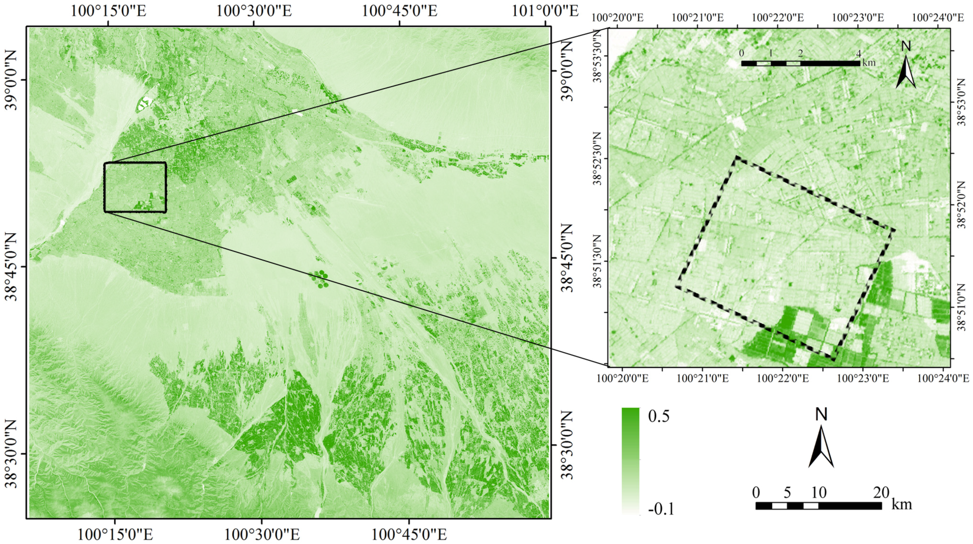
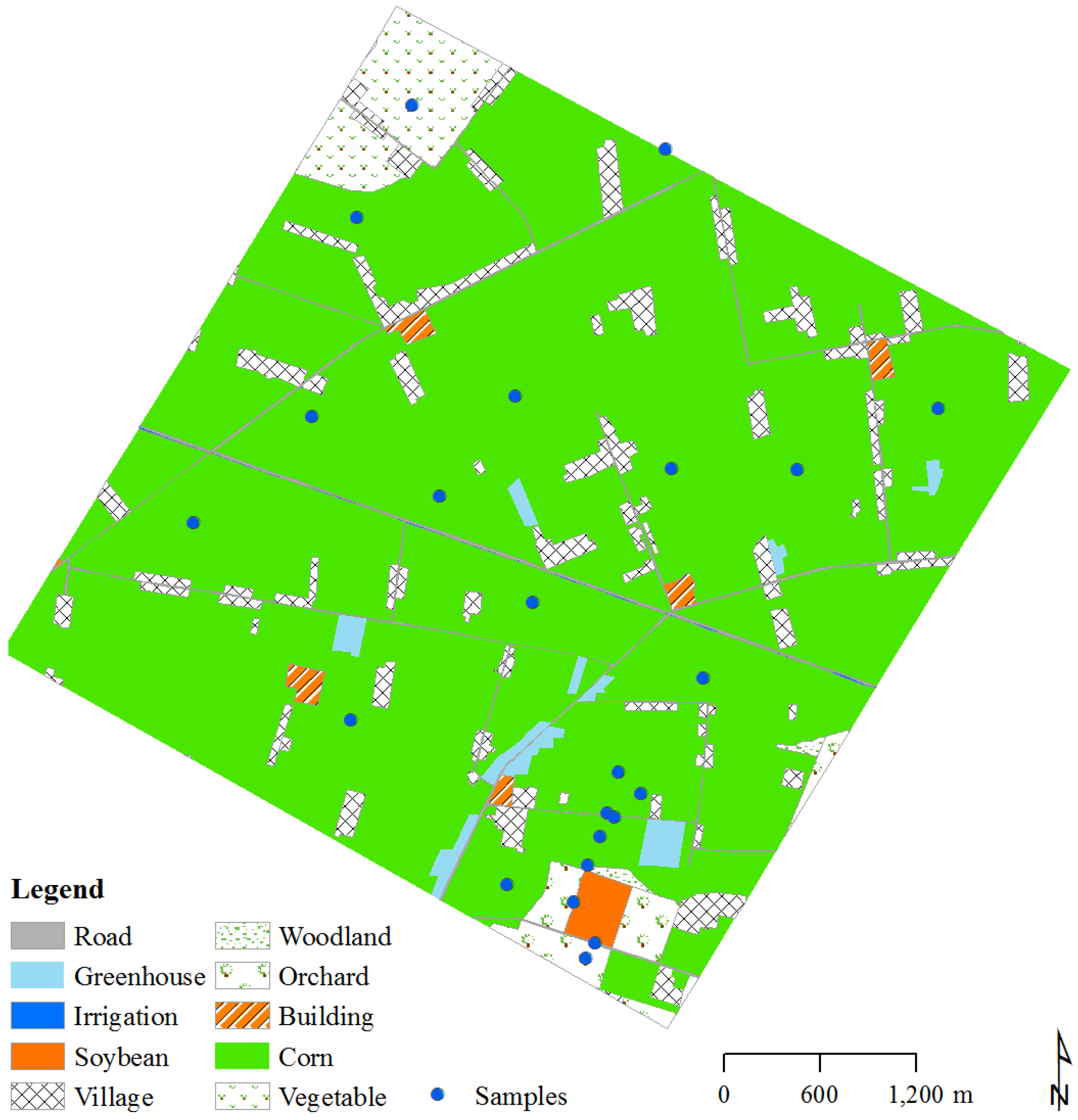
2.2. Study Site and in Situitalic> Data Measurements

The FVC data were measured at the Heihe River Basin of China during the growing period of corn, the dominant vegetation type in this area, from May to September 2012. The Heihe River is the second longest inland river in China. Comprehensive field experiments used to reveal eco-hydrological processes were conducted in the Heihe River Basin, a typical arid region of China [8,9]. The FVC data involved in this paper were collected by HiWATER [9], which is one of these experiments.
The main land cover type in this region is an artificial oasis. An NDVI map of this region acquired on 30 May shows clear boundaries between the desert and oasis (see the larger image in Figure 2). The 5 × 5 km2 kernel area of the experiment (see the area surrounded by the dashed lines in the right frame of Figure 2) is centered on the middle stream of the Heihe River Basin. Various land cover types form the strata. Corn is the dominant vegetation type in the study region, which consisted of approximately 72% agricultural land, 24% impervious surface, and 4% woodland and fruit orchard. Planted in April, the corn was still short on 30 May, thereby corresponding to low NDVI values in Figure 2. Although the croplands cover large areas of the study region, more than 30 villages are dispersed in this area and are the main influences of the spatial variability. FVCs of the impervious surfaces are nearly zero, whereas other land cover types have highly variable FVC values in terms of the vegetation seasonality. In addition, the intrinsic pattern of the cornfields varies with the irrigation schedules and other field crop managements. Therefore, the intra-pixel spatial variability of the coarse-resolution pixels in this area is considerable.
Figure 2. Normalized difference vegetation index (NDVI) map of experimental area on 30 May 2012. This map was generated from Advanced Spaceborne Thermal Emission and Reflection Radiometer (ASTER) data over the area at a resolution of 15 m. The experimental area is surrounded by the black dashed lines in the right frame.
Remotesensing 07 15817 g002
The ground measurements were taken in 23 plots (Figure 3). Each plot covers an area of 10 m × 10 m in the cropland and 30 m × 30 m in the fruit orchard and woodland. The land cover map used in this study had a spatial resolution of 30 m and an overall classification accuracy of over 90% in the experimental area [35]. The number of plots with different land cover types was determined roughly according to the area ratios of land cover types to the entire area. This approach could improve the representativeness of in situ FVCs for the generation of reference FVCs over the entire region. Sampling plots were clustered at the south corner because we attempted to test the densely distributed sampling in that area (in Section 3.2.2).
The field patch is usually larger than 2 × 2 ASTER pixels with the same agricultural management activities and homogeneous vegetation growth status. Therefore, the plot scale (10 m) may represent the scale of an ASTER pixel (15 m), and the geometric co-registration error from field measurements to ASTER data was effectively reduced.
The FVC of each sampling plot was computed using nine photographs, wherein each photograph covered approximately 2 m × 2 m. The photographs were taken along the diagonal lines across the plot. Generally, there were four 2-m intervals between photographs along a diagonal line, and only one photograph was shot for the overlapping section at the cross point of the two diagonals. A digital camera was used to image downward for crops. For fruit trees, the vegetation was photographed in a bottom-up manner, and images of the grass beneath the trees were also obtained. Details of the digital photography measurements can be found in reference [14,36]. The FVC of each photo was extracted using a published algorithm [37] that supposed that the green vegetation and background distributions of the greenness component in the color space were Gaussian; then, image segmentation was performed based on this assumption. A previous study suggested that this method obtains a stable absolute error of less than 0.05 (with an FVC range of 0 to 1) [38].
Figure 3. In situ sample plots of FVC measurements, implemented in the Heihe River Basin in 2012. Among these samples, 18 plots were located in cornfields, and the other five plots were located in a soybean field, woodland, orchard, wheat field (quite a small area, not shown in the legend) and vegetable field.
Remotesensing 07 15817 g003

2.3. Generation of Reference FVC

The ASTER L1B radiance data were used to bridge the ground measurements and coarse satellite data. ASTER data have a spatial resolution of 15 m. Prior to the regression of the ASTER NDVI and field-measured FVC, the radiance acquired at the top of atmosphere should be transferred to the surface reflectance and processed to determine the vegetation index. The atmospheric effect was corrected with Second Simulation of the Satellite Signal in the Solar Spectrum (6S) [39]. The in situ aerosol optical depth (AOD) measured during the satellite overpass with a sun photometer and the MODIS AOD product were used as the data sources for AOD. The ASTER NDVI data were geometrically corrected using a reference map to ensure that the ASTER images matched the field-measured FVC.
An empirical transfer function was required to transfer NDVI to FVC. Both linear [40] and non-linear [41,42] regressions of NDVI versus FVC obtained good agreements. The best fit for NDVI-FVC relationships depends on the vegetation types; linear fitting is not always suitable. Therefore, we chose a flexible form to combine the linear and non-linear conditions as proposed in [14]:
F V C = ( a N D V I + b ) k
where FVC and NDVI denote the in situ FVC and corresponding ASTER NDVI, and a, b and k are unknowns, which are obtained by fitting the FVC and NDVI data according to the least squares method. k indicates a linearity of FVC to NDVI. When k is approximately 1, NDVI and FVC linearly correlate, whereas k ≠ 1 corresponds to a non-linear form.
Regressions were performed in five time phases covering the beginning, rapid growing, peaking and descending stages of the corn. After the coefficients in Equation (1) were acquired, the FVC maps of the ASTER data were generated by applying the coefficients to each pixel value of the ASTER NDVI. The reference values of the coarse-resolution data were calculated by aggregating the high-resolution ASTER FVC. The uncertainty of fitted ASTER FVC can be reduced during upscaling when random errors are canceled out during aggregation, therein benefiting the performance analysis of the sampling methods.
Table 1 illustrates the coefficients of determination (R2) and the root mean square error (RMSE) of the NDVI and FVC over five time phases. We can see that the RMSE is generally less than 0.031 when data acquired over a single time phase are used in the regression. However, if all the data obtained over five time phases are used to fit one transfer function, the RMSE will be 0.072.
Table 1. The statistical parameters related to the regression of Advanced Spaceborne Thermal Emission and Reflection Radiometer (ASTER) fractional vegetation cover (FVC). R2 is the coefficient of determination of ASTER Normalized Difference Vegetation Index (NDVI) and field-measured FVC; k is the degree of non-linearity in Equation (1); RMSE refers to the root mean square error between ASTER NDVI and the field-measured FVC; and FVCavg and FVCdev are the averages and standard deviations of the field–measured FVC, respectively.
Date30 May 201224 June 201210 July 201211 August 201212 September 2012ALL *
R20.9830.8500.9280.9110.9470.914
k1.2321.1360.3280.4591.2990.523
RMSE0.0200.0200.0160.0310.0100.072
FVCavg0.1810.6230.6900.7200.1330.469
FVCdev0.1680.0530.0900.0870.0400.276
* ALL represents the situation in which data obtained over all five time phases are used in the regression.

3. Methodology

3.1. Sampling Methods

In this research, four sampling methods were applied to validate a remote-sensing product: simple random sampling, stratified sampling, ordinary kriging spatial sampling and MSN spatial sampling. Simple random sampling and stratified sampling are two important sampling methods applied in both non-spatial- and spatial-related research. The samples were assumed to not be autocorrelated for the sample number calculation and population estimation [43,44]. The ordinary kriging and MSN-based spatial sampling methods consider spatial autocorrelation in geographical phenomena, and they use a variogram model to describe the relationship between phenomenon similarity and spatial distance [34,43].
Kriging is a spatial interpolation method based on regionalized variable theory. When a number of samples are collected, the value of an un-sampled location can be estimated by a linear combination of samples. The samples weights are determined using the regional semi-variogram and distances between the unknown point and samples, which are solved from the following linear equations [43].
j = 1 n w j C i j + μ = C i 0 ( i = 1 , , n )
j = 1 n w j = 1
y ¯ = i = 1 n w i y i
σ ˜ R 2 = σ ˜ 2 ( i = 1 n w i C i 0 + μ )
where n is the sample number, wj is the jth sample’s weight, Ci0 is the covariance between the ith sample and the unknown point, Cij is the covariance between the ith sample and the jth sample, μ is the Lagrange multiplier, σ ˜ 2 is the variance, and y ¯ and σ ˜ R 2 are the estimated mean and error variance, respectively. The covariance C can be calculated from a semi-variogram function fitted from samples or historical data. The objective of the kriging method is to minimize the error variance. For a given sample number, the locations of samples can be determined using optimization algorithms [23,24].
A coarse pixel in the remote sensing image is treated as a large block. Samples located in research regions will be used to estimate the pixel value using ordinary kriging. Then, Ci0 in Equation (2) is the average covariance between the ith sample and all unknown points in the region. Due to the high correlation between NDVI and FVC, we use NDVI product as a proxy to fit the semi-variogram and sample optimization. When the semi-variogram function is fixed, the estimated error variance of the unknown point or region is only determined by the spatial configurations (distance and direction) of collected samples. A Monte-Carlo-based simulation method is adopted to select a group of samples with minimum theoretical estimated error variance. An iteration process is repeated until the error variance does not decrease or the maximum number of iterations is reached. The maximum number of iterations is 30,000.
The MSN model is an integration of stratified sampling and ordinary kriging that considers both spatial heterogeneity and spatial autocorrelation. The intrinsic assumption requires that the region is homogeneous to enable ordinary kriging estimation to be applied. A heterogeneous region is separated into several small regions to be estimated, and then, the results are summed with area weights. Nevertheless, the separation does not consider potential spatial autocorrelations between different small regions, which would decrease the estimation accuracy. In the MSN method, strata are used to separate the heterogeneous field into small homogeneous fields. Semi-variograms model the spatial autocorrelations in the small fields. A global semi-variogram will be fitted if objects in different strata autocorrelate. For ground containing different crop and land-use types, such as corn, soybean and woodland, each type is treated as a stratum, and the spatial autocorrelation will be modeled in each stratum. The sample weights are solved from Equations (6) and (7) [34]. The estimated pixel-scale mean value, y ¯ , and its variance, σ ˜ 2 , are expressed as Equations (8) and (9):
a p h = 1 H i = 1 n h a h w h i C ( y h i , y p j ) + μ p = a p 1 C ( y p j , y ( s ) ) d s
i = 1 n h w h i = 1
y ¯ = 1 h = 1 H h i = 1 n h w h i y h i
σ ˜ 2 = 2 C ( y ( s ) , y ( s ) ) d s d s 1 h = 1 H i = 1 n h a h w h i C ( y h i , y ( s ) ) d s h = 1 H μ h
where H (h = 1, …, H; p = 1, …, H) is the number of strata; nh is the sample number in the hth stratum; yhi is the ith sample in the hth stratum, with whi being its weight, which is solved from the MSN model; and h are the areas of the pixel and the hth stratum; a h = h / ; μh is the Lagrange multiplier; y ( s ) denotes the sample at location s; and C ( y ( s ) , y ( s ) ) is the covariance between the sample y ( s ) and the sample y ( s ) . Similar to kriging, we also used the MSN model to optimize the sampling by minimizing the error variance σ ˜ 2 with an annealing simulation [24]. This method attempts to determine the most appropriate sample number and spatial locations to minimize the variance via a Monte Carlo simulation similar to that in the above kriging sampling method.
The process includes three main steps. First, for a given sample number m, m initial spatial samples are generated using a simple random sampling method. Each stratum should have at least two samples for solving Equations (6) and (7). Second, sample locations are adjusted individually to generate new spatial configurations of samples. For each new sample configuration, the theoretical estimation variance will be calculated according to Equation (9). The configuration with the smallest theoretical estimated error variance will be kept. Third, the second step is repeated with a Monte Carlo simulation algorithm to find the sample configuration with the smallest theoretical estimated error variance. The iteration process attempts to select a group of samples with minimum theoretical estimated error variance calculated by the MSN method. This is repeated until the error variance does not decrease or the maximum number of iterations, namely, 30,000, is reached.

3.2. Design of Experiments

This test attempts to evaluate the sampling methods with two designed experimental scenes. To be realistic, all the designed schemes were tested based on the criterion of the highest accuracy of the FVC estimation with the smallest number of sampling points. In reality, the positions of samples remain constant in an experiment to ensure the stability of validation. Therefore, the estimation errors of a long period (at least when the experiment was being conducted) should be considered when designing the sampling method. We performed the tests when samples remained at the same positions in five temporal stages. The alternative sampling methods generally require ASTER NDVI data and land cover maps to calculate the locations of the sampling plots.

3.2.1. Sparse Sampling (Scene 1)

The first scene (referred to as Scene 1) consisted of “sparsely” distributed samples used to validate pixels at resolutions of 1 km over the entire experimental area. This scene may represent the situation when field campaigns are conducted in a large area with limited samples. In the designed scene, the positions of 9 samples (the red samples in Figure 4) were varied according to the sampling method, whereas the positions of another 13 samples (in blue in Figure 4) were fixed. In the sample location optimization process, the positions of the 13 fixed samples were not changed. The remaining 9 samples were initially selected by simple random sampling in both MSN and ordinary kriging. Then, the positions of the 9 samples were adjusted step-by-step using a Monte Carlo simulation to minimize the theoretical estimated error variance. After the locations and weights of all the pixels were determined by the sampling methods, the FVC values of the samples were summarized to estimate the FVC at the resolution of 1 km, which represents the resolution of typical coarse-resolution products (e.g., the MODIS product). The estimated value of each grid was calculated by multiplying weights by the values of the samples. Figure 4 shows the sampling positions derived using MSN and ordinary kriging method. The simple sampling method and stratified sampling method were not performed in Scene 1. The prerequisite conditional to operate these two methods, i.e., each grid should have at least one sample, were not met in our sparse sampling scene.

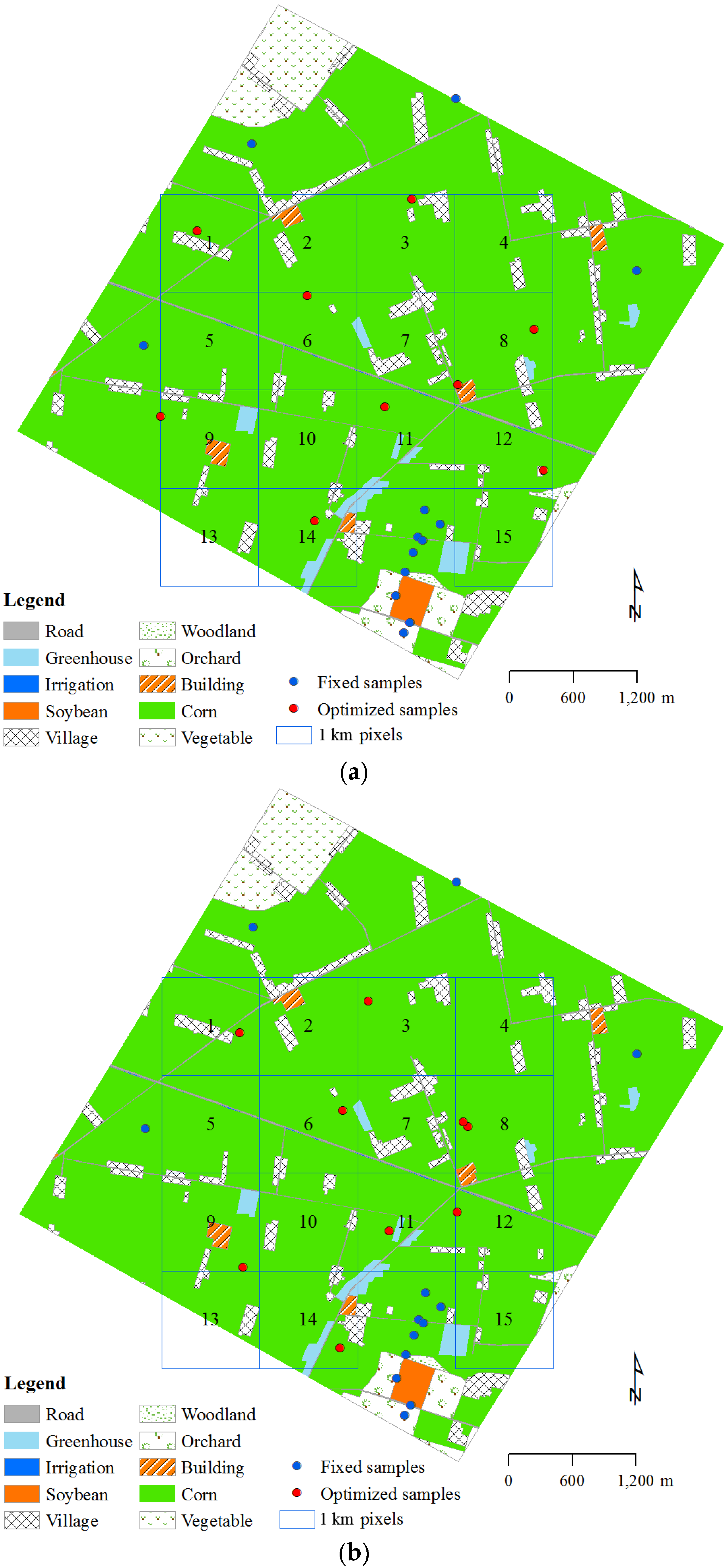
3.2.2. Dense Sampling (Scene 2)

The other scene (referred to as Scene 2) consisted of “densely” distributed samples. A rectangular region of approximately 1.5 km × 2 km (red rectangular region in Figure 5) was chosen as the region of interest to test the four sampling methods mentioned in Section 3.1. This scene was composed of fruit trees, corn, villages, soybeans, greenhouses, and rich types of land cover classes, and the samples were densely distributed. The designed scene may represent a typical case of a field campaign with sufficient numbers of samples in various class types. The MSN method and the original kriging method were used to determine the positions of 10 samples and the corresponding weights attributed to the samples. As for the simple random sampling and stratified sampling methods, the sampling positions varied with the random number selected in their implementation. Therefore, we applied these two methods 100 times and collected all the data for comparison. The FVC values estimated using the sampling methods were contrasted to the mean of the reference FVC of the entire rectangular region. Scene 2 was also selected for the comparison of the MSN and other sampling methods with changing numbers of samples. Different methods were used to compute the weights of samples with fixed sampling positions and test the average absolute errors of estimation after running 5000 simulations.
The major difference between Scenes 1 and 2 is the distances between samples that were utilized to estimate the coarse-resolution FVC. In Scene 2, the density of samples is relatively high.
Figure 4. Distributions of fixed and optimized samples in the sparsely distributed scene using the mean of surface with non-homogeneity (MSN) method (a) and the ordinary kriging method (b). Coarse pixels in (a,b) marked as Nos. 1–15, have a resolution of 1 km.
Remotesensing 07 15817 g004
Figure 5. Distributions of the fixed and optimized samples in the dense sampling scene calculated using the MSN method (a) and the ordinary kriging method (b) (in the red rectangular region).
Remotesensing 07 15817 g005

3.3. Scaling Bias of FVC Estimates

The NDVI, FVC and other parameters could be considered as random variables from a statistical point of view. If the calculation of the sampling is only based on the NDVI space, then the estimated FVC and reference FVC of a coarse pixel will show a bias when the relationship between FVC and NDVI is non-linear. Therefore, the optimization sampling scheme for NDVI is not optimal for FVC. The bias varies with the expectation and variance of NDVI.
In the present study, we simplified the problem and used a single formula to describe the bias or so-called “scaling effect” without considering the different vegetation types. A Taylor expansion was used to obtain an approximate form of the deviation involving many parameters [45,46,47]. The second-order Taylor expression can mathematically describe the expectation of a function f as follows:
E ( f ( X ) ) f ( μ x ) + f ( μ x ) 2 σ X 2
where μ x is the expectation of the random variable X, f denotes the function that transfers X to another variable, and σ X 2 is the variance of X. Thus, f ( μ x ) 2 σ X 2 is the bias, which is influenced by the variance of the variable and non-linear form of the function f. Combining Equations (1) and (10) easily yields the bias of the expected FVC and the FVC transferred from the expected NDVI:
B ( μ N D V I , σ N D V I 2 ) = a 2 k ( k 1 ) ( a μ N D V I + b ) k 2 2 σ N D V I 2
where μ N D V I and σ N D V I 2 are the expectation and variance of NDVI in an experimental area, respectively.

4. Results and Analysis

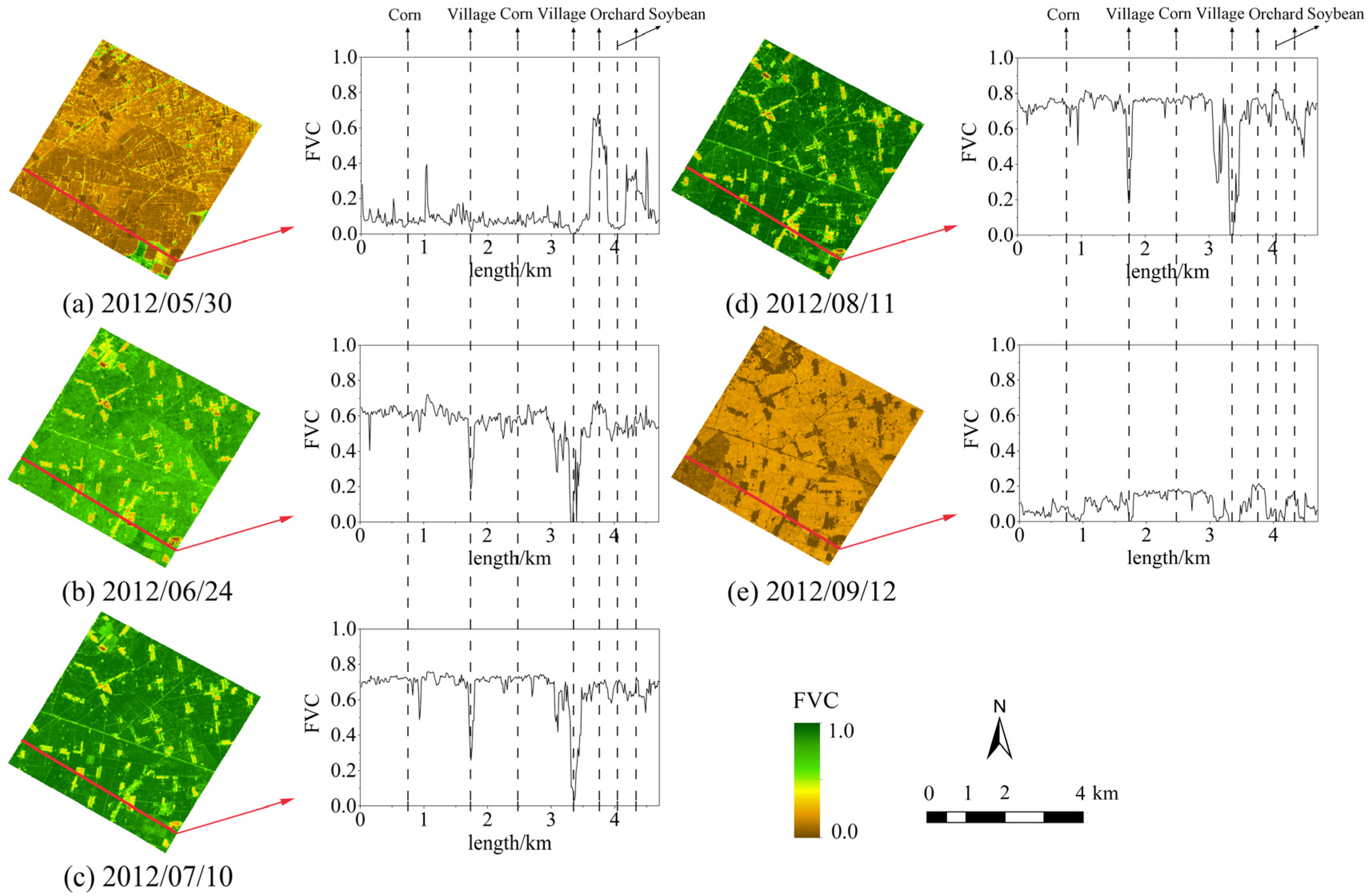
4.1. Spatial and Temporal Pattern of ASTER FVC

Figure 6 shows the spatial patterns of ASTER FVC and phenological variability of vegetation. One factor influencing the spatial heterogeneity is the contrast between impervious surfaces and vegetated areas. In general, the FVC values of artificial impervious surfaces (e.g., villages) remained at a low level during all the growth stages of vegetation. The contrast between the FVCs of the two land cover types became notable when vegetation grew to achieve a high level of FVC (Figure 6b–d). The difference between the two FVCs was up to 0.7 as the plants flourished in August (Figure 6d).
Figure 6. (ae) Spatial distributions of ASTER FVC in different growth stages (15-m resolution). In each growth stage, the FVC profile along the transect line (red line) is demonstrated.
Remotesensing 07 15817 g006
In addition, Figure 6 shows that the differences between crops and fruit trees also strongly influence the spatial heterogeneity. The FVCs of vegetated areas, i.e., croplands and orchards, fluctuated depending on the vegetation seasonality. The corn started to grow at the end of May, when fruit trees had passed the stage of rapid leaf growth. The FVC of corn was at the same level as the FVC of fruit trees after the rows almost achieved canopy closure in June. The difference between the two FVCs was considerable in May (Figure 6a) and indistinctive when the FVC reached its peak in August (Figure 6d). Correspondingly, these temporal changes remarkably affect the spatial variability.
Table 2 shows that the degrees of non-homogeneity in the study area (standard deviations of 15 m FVC in Scene 1) increase and then decrease corresponding to the planting, closing and harvest of the irrigated crops. As mentioned above, at the early stage of growth, cornfields showed a low FVC value, which was similar to the FVC of non-vegetation areas and caused the land surface to be relatively homogeneous. The deviations increased in August, when corn grows to a high level of FVC. In Scene 2, a particularly large spatial variability on 30 May was found due to the prominent difference between cornfields and orchards.
Table 2. The standard deviations of ASTER FVC over the study regions in Scenes 1 and 2.
Date30 May 201224 June 201210 July 201211 August 201212 September 2012
Scene 10.0680.1020.1040.1300.053
Scene 2 0.1970.1070.1060.141 0.057

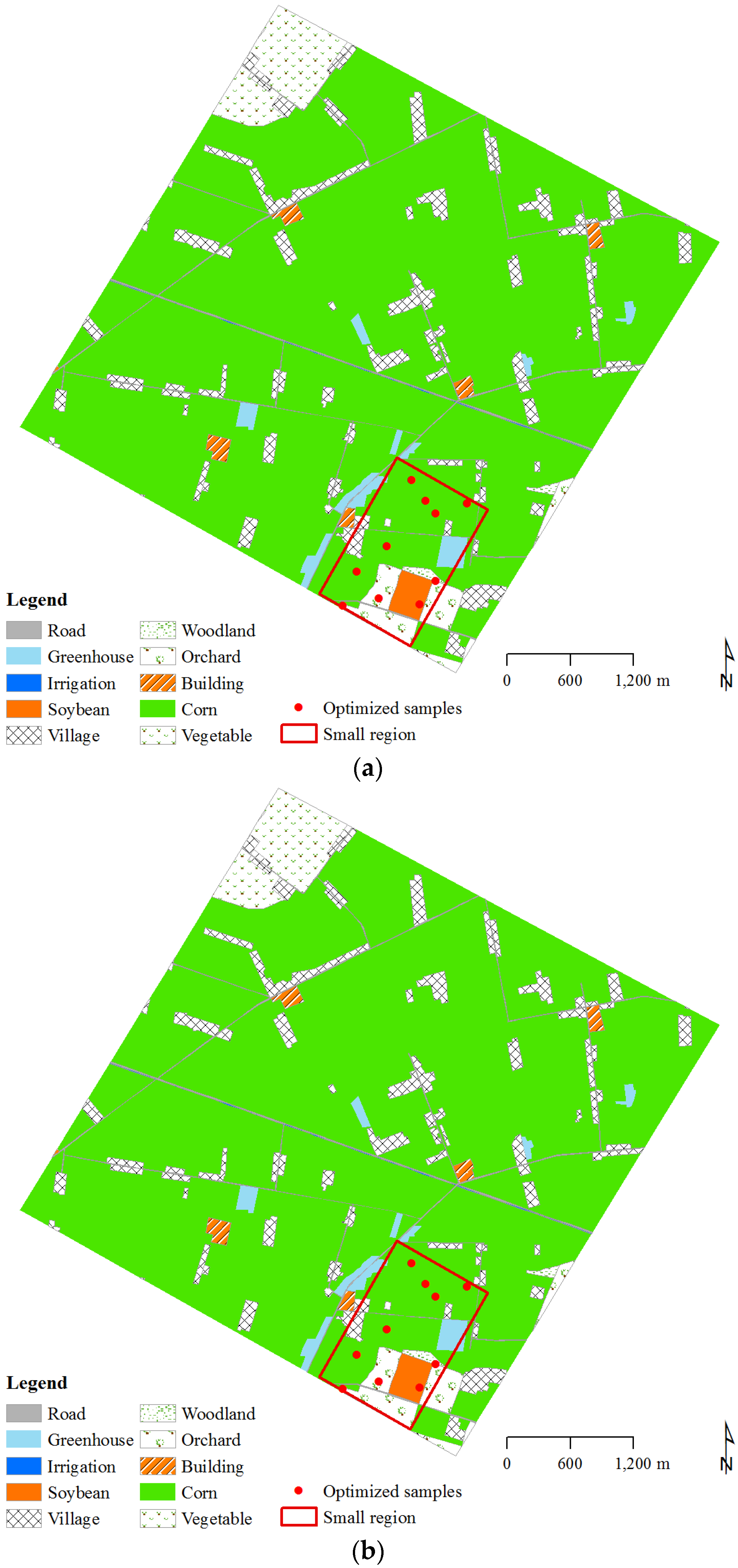
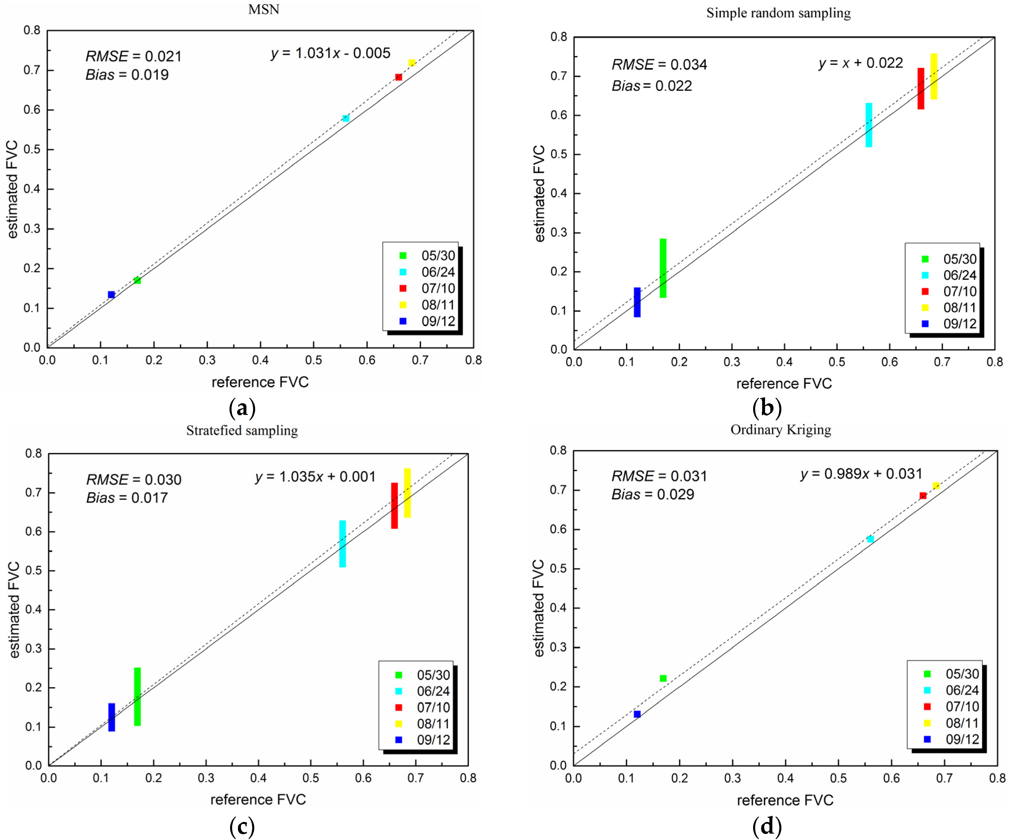
4.2. Sparsely Distributed Samples

The MSN method and ordinary kriging method were used to compute the locations of nine movable samples and the weights of 22 samples in each time phase. The scattering plots of the reference FVC and estimated FVC of the 1-km-resolution grids are shown in Figure 7. In general, the data points are mainly distributed around the y = x line for both of the methods. The FVC estimates on the coarse scale strongly correlate with the reference FVC. On all five dates, the estimates show slightly positive deviations from the reference FVC values. The FVC was estimated using the MSN method with a bias of 0.018 and RMSE of 0.030, and the ordinary kriging method results in larger bias and RMSE of 0.028 and 0.036, respectively (Figure 7). In addition, half of the samples were located in the rectangular region of Scene 2. Table 2 shows that the spatial variability of FVC was large on 30 May for Scene 2 and small on 12 September, corresponding to the outlier data points on 30 May and good accuracy on 12 September in Figure 7.
Figure 7. Scattering plots of reference FVC and estimated FVC using the MSN method (a) and the original kriging method (b) at a scale of 1 km (Scene 1).
Remotesensing 07 15817 g007

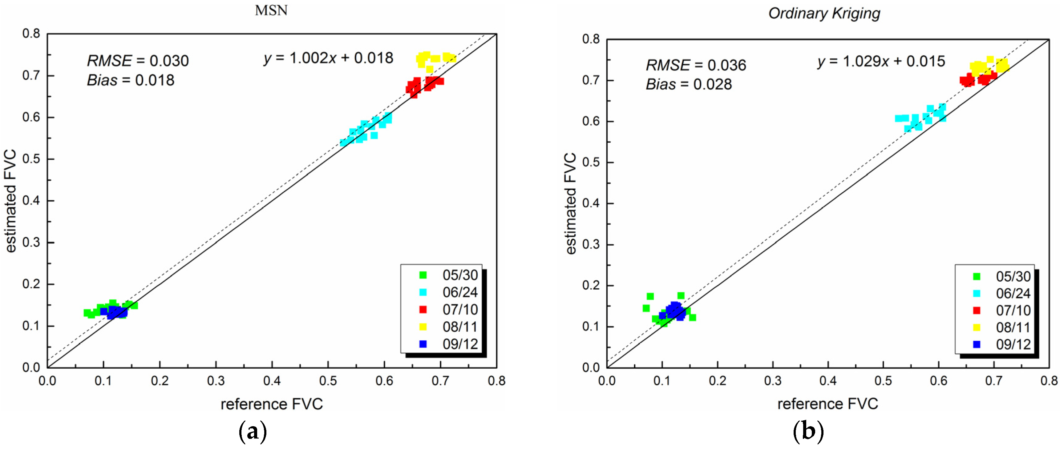
4.3. Densely Distributed Samples

In Scene 2, the errors of the estimated FVC are comparable to those in Scene 1. The four sampling methods demonstrate a RMSE of generally less than 0.035 (Figure 8). The MSN method considers spatial heterogeneity in and between strata, resulting in an RMSE of 0.021, which is the smallest among the four methods. The stratified sampling method performed better on 30 May than the simple random sampling and ordinary kriging methods, when the contrast between cornfields and orchards was prominent. The smallest bias was also found when applying the stratified sampling method, suggesting that the spatial heterogeneity was highly correlated to land cover type.
Figure 8. Scattering plots of reference FVC and estimated FVC using the MSN (a); simple random sampling (b); stratified sampling (c); and ordinary kriging (d) methods over an area of 3 km2 (Scene 2). The simple random sampling and stratified sampling methods were applied 100 times.
Remotesensing 07 15817 g008
Nevertheless, the results of the simple random and stratified sampling methods in Figure 8 reflect the averages of 100 executions. In practice, the performances of these two methods could be worse.

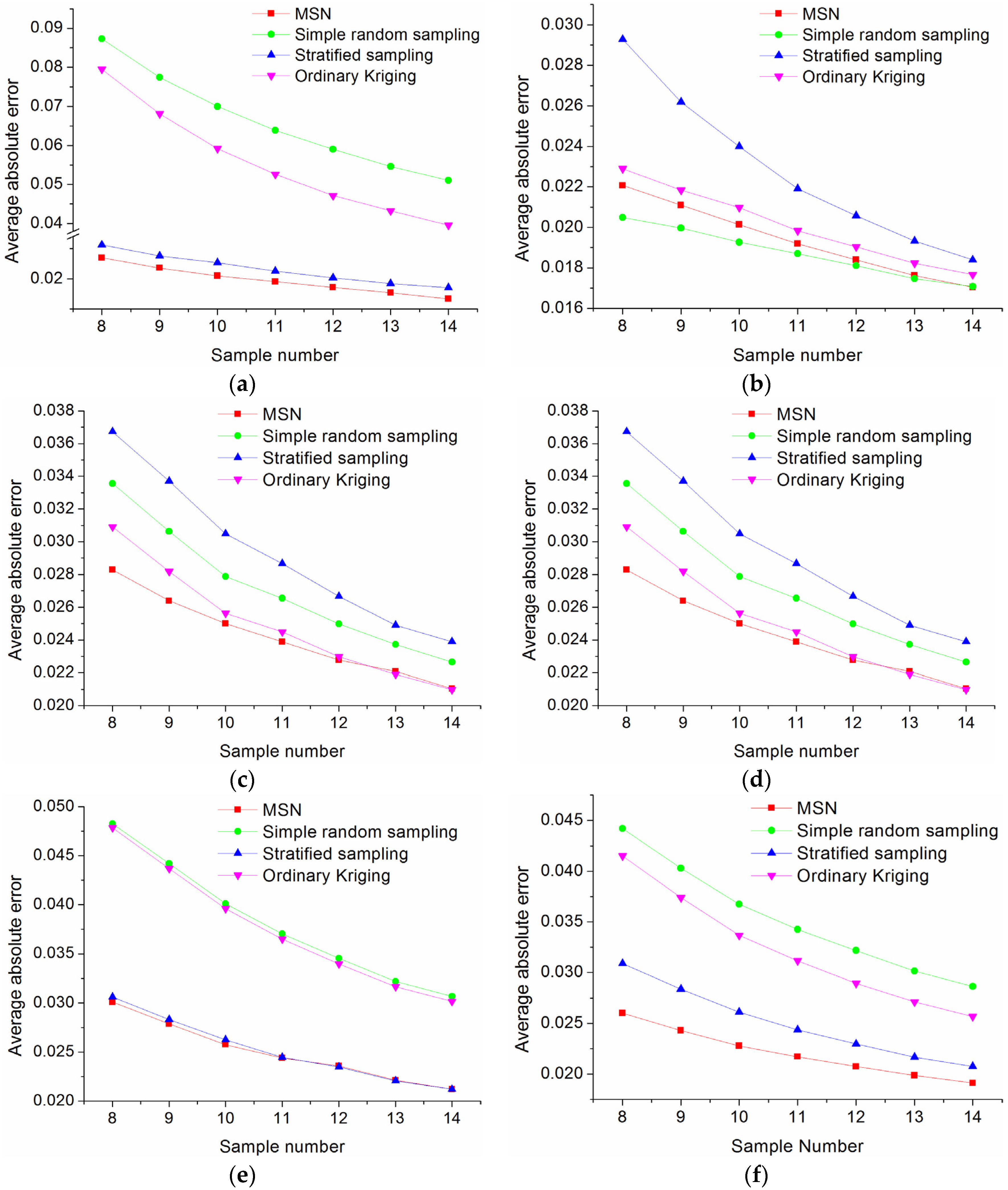
4.4. Evaluation of Sampling Methods with Changing Number of Samples

We selected Scene 2 to test the MSN and other sampling methods in response to the changing number of samples. Generally, the methods that considered both heterogeneity and autocorrelations between strata (e.g., the MSN method) are superior to the other methods. Among the sampling methods, MSN demonstrated its advantage by providing the smallest errors of estimation (Figure 9).
The errors of FVC estimates, regardless of the applied sampling method, will gradually decrease and become similar when the number of samples increases. Most of the sampling methods achieve an accuracy of approximately 0.02 to 0.03 with a sample number of 14, except for the simple random sampling and ordinary kriging methods on 30 May. The uncertainty level and sensitivity of the error to the sample number on 30 May is relatively high compared to those on other dates because of the high spatial variability (Table 2).
Figure 9. Averages of absolute errors of FVC generated by applying different sampling methods in Scene 2 with increasing sample numbers: (a) 30 May; (b) 24 June; (c) 10 July; (d) 11 August; (e) 12 September; and (f) average errors of FVC over all the time phases.
Remotesensing 07 15817 g009
However, the accuracy of each algorithm varies in the temporal range, which is consistent with the changing spatial variability in the growth stages of vegetation. The contrast between the FVC values of different land cover types is maximized at the initial stage of corn growth (May) and is minimized as the growth is saturated (June, July and early August), corresponding to the temporal patterns of corn and fruit trees (Figure 6). This means that the spatial variability in this area is dominated by the heterogeneity between strata in May and September (Figure 9a,e) and by the spatial autocorrelation from June to August (Figure 9b–d). Therefore, the methods that consider heterogeneity between strata (stratified sampling and MSN) perform well in Figure 9a,e, whereas the ordinary kriging method and the MSN method provide good accuracy in Figure 9b–d. In most of the cases, the simple random sampling method generates large errors compared to other methods.

5. Discussions

The parameter of interest in this paper, i.e., green vegetation FVC, is relatively stable and predictable compared with rapidly changing variables such as temperature, radiation and evaporation. Given that FVC has a linear or quasi-linear relationship with NDVI [36], tests are facilitated when NDVI maps are assumed to be known in advance. In practice, prior to the design of each experiment, the NDVI maps of the region may be extracted from satellite data obtained in recent years. The locations and weights of samples can be determined based on the NDVI statistics. The variance of FVC (C in Equations (2), (5), (6) and (9)) can simply be estimated by a given linear transformation or even replaced by that of NDVI because FVC and NDVI have nearly the same range of values. However, according to Equation (10), slight scaling biases may also exist in FVC estimations with a non-linear NDVI-FVC relationship at heterogeneous surfaces.
Given the NDVI averages and variances over the study area, the scaling biases between estimated and reference FVC were calculated using Equation (11). The predicted biases were then compared with the real biases between the reference FVC and its estimates (Table 3).
Table 3. Predicted scaling biases (Bias_Pred) and the real biases (Bias_Real) of the estimated FVC using the MSN method.
Date30 May 201224 June 201210 July 201211 August 201212 September 2012
Scene 1
Bias_Pred−0.0040.0000.0060.011−0.005
Bias_Real0.0090.0080.0300.0230.007
Scene 2
Bias_Pred0.0370.0100.0100.0130.015
Bias_Real0.0000.0340.0270.0070.008
Table 3 indicates that the theoretical biases between the reference FVC and the estimated FVC are realistically small. The scaling bias is not easily distinguished from the remaining errors. However, the positive or negative trend of the predicted biases in Table 3 is consistent with that of the real biases when the values of the absolute deviations that are less than 0.01 are ignored (four cases remain: 10 July and 11 August in Scene 1 and 24 June and 10 July in Scene 2). It should be noted that the scaling effect discussed in the current paper only concerns the transfer from high-resolution NDVI to FVC; specifically, the scaling effect generated from NDVI itself [48,49], which may affect the use of coarse-resolution NDVI, is beyond the scope of this study.
The uncertainty of reference FVC mainly depends on the field measurements and ASTER NDVI. The fit between them resulted in residual errors, which indicated an RMSE of less than 0.031. The error of ASTER FVC can be further reduced in the aggregation of ASTER FVC, which makes the uncertainty of reference coarse-resolution FVC smaller than the differences among sampling methods. Therefore, the general trends deduced from the comparison of reference data and estimated data at coarse resolutions are believed to be reliable.
In the MSN method, the sampling problem can be solved through an optimization process, where the variance, autocorrelations, and other statistics are known a priori to a certain extent. If the number of samples is constant, then optimal sampling schemes can be obtained to guarantee minimal estimation errors. The MSN method represents an optimization scheme that has been established in spatial statistics. Simple random sampling is inefficient when the investigated ground surface has spatial autocorrelation or strata. Ordinary kriging sampling performs well in increasing the estimation accuracy when the ground surface is relatively homogenous. However, for a more complicated surface, stratification is necessary in sampling and estimation. The MSN method requires the designated attributes of strata and the covariance of strata as input data, which are supplied by introducing land cover data and several prior statistics. Although the MSN method optimizes the use of NDVI and land cover types, it also introduces a certain type of risk. The method that yields the most accurate estimation may not be the most stable one. Thus, redundant samples are necessary from a pragmatic perspective. The weight of a single sample is not suggested to be large, which guarantees a reasonable estimation even if unpredictable errors exist in this sample.

6. Conclusions

Sampling methods are often applied to present an estimation of the coarse pixel mean in the ground-based validation of remote sensing products. In this study, we designed tests to evaluate sampling methods for the estimation of FVC at coarse resolutions. This research attempts to find suitable sampling methods for the validation of FVC products and provide recommendations for the design of field experiments. The MSN and other conventional sampling methods are employed for comparison.
The spatial variability of the study region primarily depends on the contrast between strata and the spatial autocorrelation and varies with the growth of different types of vegetation. The performance of the different sampling methods varies based on their model assumptions. In our tests, the stratified sampling and kriging methods perform well when the heterogeneity between and in strata dominate the spatial variability, respectively. Nevertheless, the methods that consider both spatial heterogeneity and correlations in and between strata are more accurate over the vegetative growth cycle and require fewer samples. The MSN method demonstrates its advantage of considering these factors. The tests presented in this paper illustrate that the errors of FVC estimated using the MSN method are approximately less than 0.03 in the two designed scenes. In general, the MSN method is recommended for the determination of the locations and weights of samples when field campaigns are conducted to validate remotely-sensed FVC products.
For the validation of FVC, NDVI or other vegetation indices represent convenient tools for providing a preliminary estimate. Moreover, FVC shows a good linear correlation with NDVI, and the estimations may remain nearly unbiased, thereby ensuring that the preliminary estimation is not difficult. The scaling effect is generally insignificant when transferring from NDVI to FVC.

Acknowledgments

This work was supported by the National Basic Research Program of China (973 Program) (No. 2013CB733402), the key program of NSFC (No. 41331171 and 91125004), the National High Technology Research and Development Program of China (No. 2012AA12A305), and the program of NSFC (No. 41301425). The authors thank all those who contributed to the data measurements: Shuzhen Jia, Yuanxin Jia, Liying Geng, and Wenping Yu from the Cold and Arid Regions Environmental and Engineering Research Institute, Chinese Academy of Sciences; Yongsheng Huang from Northwest Normal University; and Jing Zhao, Yiming Chen, Jiqiang Zhao, Kai Yan, Yan Wang, Zhonghu Jiao, Ronghai Hu, and Yun Li from Beijing Normal University. The ASTER radiance data were provided by NASA. The authors would like to thank the four anonymous reviewers for their comments and suggestions.

Author Contributions

Xihan Mu proposed the idea of testing different sampling methods for FVC products and designed the structure of this manuscript. Maogui Hu guided the research work related to the MSN and other sampling methods. Wanjuan Song and Gaiyan Ruan prepared FVC data and edited the manuscript. Yong Ge and Jinfeng Wang provided suggestions on the sampling methods used in this study. Shuai Huang helped revise the manuscript. Guangjian Yan suggested the assessment of the scaling bias of FVC.

Conflicts of Interest

The authors declare no conflict of interest.

References

  1. Ge, Y.; Li, X.; Hu, M.G.; Wang, J.H.; Jin, R.; Wang, J.F.; Zhang, R.H. Technical specification for the validation of remote sensing products. Int. Arch. Photogramm. Remote Sens. Spat. Inf. Sci. 2013, XL-2/W1, 13–17. [Google Scholar] [CrossRef]
  2. Li, X.; Wang, S.G.; Ge, Y.; Jin, R.; Liu, S.M.; Ma, M.G.; Shi, W.Z.; Li, R.X.; Liu, Q.H. Development and experimental verification of key techniques to validate remote sensing products. Int. Arch. Photogramm. Remote Sens. Spat. Inf. Sci. 2013, XL-2/W1, 25–30. [Google Scholar] [CrossRef]
  3. Justice, C.O.; Tucker, C.J. The Sage Handbook of Remote Sensing:Coarse Spatial Resolution Optical Sensors; SAGE Publications Ltd.: London, UK, 2009; pp. 139–151. [Google Scholar]
  4. Baret, F.; Weiss, M.; Allard, D.; Garrigues, S.; Leroy, M.; Jeanjean, H.; Fernandes, R.; Myneni, R.; Privette, J.; Morisette, J. VALERI: A Network of Sites and a Methodology for the Validation of Medium Spatial Resolution Land Satellite Products. Available online: http://w3.avignon.inra.fr/valeri/documents/VALERI-RSESubmitted.pdf (accessed on 26 August 2015).
  5. Campbell, J.; Burrows, S.; Gower, S.; Cohen, W. Bigfoot Field Manual; Technical Report, DE2001-13418; NASA STI: Hampton, VA, USA, 1999. [Google Scholar]
  6. Buermann, W.; Helmlinger, M. SAFARI 2000 LAI and FPAR Measurements at Sua Pan, Botswana, Dry Season 2000; Oak Ridge National Laboratory Distributed Active Archive Cente: Oak Ridge, TN, USA. Available online: http:// daac.ornl.gov/S2K/safari.shtml (accessed on 26 August 2015).
  7. Morisette, J.T.; Baret, F.; Privette, J.L.; Myneni, R.B.; Nickeson, J.E.; Garrigues, S.; Shabanov, N.V.; Weiss, M.; Fernandes, R.A.; Leblanc, S.G.; et al. Validation of global moderate-resolution LAI products: A framework proposed within the ceos land product validation subgroup. IEEE Trans. Geosci. Remote Sens. 2006, 44, 1804–1817. [Google Scholar] [CrossRef]
  8. Li, X.; Li, X.; Li, Z.; Ma, M.; Wang, J.; Xiao, Q.; Liu, Q.; Che, T.; Chen, E.; Yan, G.; et al. Watershed allied telemetry experimental research. J. Geophys. Res. Atmos. 2009, 114, D22103. [Google Scholar] [CrossRef]
  9. Li, X.; Cheng, G.; Liu, S.; Xiao, Q.; Ma, M.; Jin, R.; Che, T.; Liu, Q.; Wang, W.; Qi, Y.; et al. Heihe watershed allied telemetry experimental research (HiWATER): Scientific objectives and experimental design. Bull. Am. Meteorol. Soc. 2013, 94, 1145–1160. [Google Scholar] [CrossRef]
  10. Mu, X.; Huang, S.; Chen, Y. HiWATER: Dataset of Fractional Vegetation Cover in the Middle Reaches of the Heihe River Basin; Beijing Normal University: Beijing, China; Cold and Arid Regions Environmental and Engineering Research Institute, Chinese Academy of Sciences: Lanzhou, China, 2013. [Google Scholar] [CrossRef]
  11. Yan, G.; Mu, X.; Liu, Y. Chapter 13—Fractional vegetation cover. In Advanced Remote Sensing; Liang, S., Li, X., Wang, J., Eds.; Academic Press: Boston, MA, USA, 2012; pp. 415–438. [Google Scholar]
  12. García-Haro, F.J.; Camacho-de Coca, F.; Miralles, J.M. Inter-Comparison of SEVIRI/MSG and MERIS/ENVISAT Biophysical Products over Europe and Africa. In Proceedings of the 2nd MERIS/(A) ATSR User Workshop, Frascati, Italy, 22–26 September 2008.
  13. Fillol, E.; Baret, F.; Weiss, M.; Dedieu, G.; Demarez, V.; Gouaux, P.; Ducrot, D. Cover fraction estimation from high resolution SPOT HRV & HRG and medium resolution SPOT-VEGETATION sensors. Validation and comparison over South-west France. In Proceedings of the Second International Symposium on Recent Advances in Quantitative Remote Sensing, Torrent (Valencia), Spain, 25–29 September 2006; pp. 659–663.
  14. Mu, X.; Huang, S.; Ren, H.; Yan, G.; Song, W.; Ruan, G. Validating GEOV1 fractional vegetation cover derived from coarse-resolution remote sensing images over croplands. IEEE J. Sel. Top. Appl. Earth Obs. Remote Sens. 2015, 8, 439–446. [Google Scholar] [CrossRef]
  15. Rooney, D.E. Human Cytogenetic: Constitutional Analysis, 3rd ed.; Oxford University Press: New York, USA, 2001; Volume 1. [Google Scholar]
  16. Black, T.R. Doing Quantitative Research in the Social Sciences: An Integrated Approach to Research Design, Measurement and Statistics; SAGE: London, UK, 1999; p. 118. [Google Scholar]
  17. Daniel, J. Sampling Essentials: Practical Guidelines for Making Sampling Choices; SAGE: Los Angeles, CA, USA, 2012; pp. 125–140. [Google Scholar]
  18. Tobler, W.R. A computer movie simulating urban growth in the detroit region. Econ. Geogr. 1970, 46, 234–240. [Google Scholar] [CrossRef]
  19. Cressie, N. Statistics for spatial data. Terra Nova 1992, 4, 613–617. [Google Scholar] [CrossRef]
  20. Haining, R.P. Spatial Data Analysis: Theory and Practice; Cambridge University Press: Cambridge, UK, 2003. [Google Scholar]
  21. Wang, J.-F.; Stein, A.; Gao, B.-B.; Ge, Y. A review of spatial sampling. Spat. Stat. 2012, 2, 1–14. [Google Scholar] [CrossRef]
  22. Groenigen, J.W.V.; Stein, A. Constrained optimization of spatial sampling using continuous simulated annealing. J. Environ. Qual. 1998, 27, 1078–1086. [Google Scholar] [CrossRef]
  23. Brus, D.J.; Heuvelink, G.B.M. Optimization of sample patterns for universal kriging of environmental variables. Geoderma 2007, 138, 86–95. [Google Scholar] [CrossRef]
  24. Hu, M.-G.; Wang, J.-F. A spatial sampling optimization package using MSN theory. Environ. Model. Softw. 2011, 26, 546–548. [Google Scholar]
  25. Hu, M.-G.; Wang, J.-F.; Zhao, Y.; Jia, L. A B-SHADE based best linear unbiased estimation tool for biased samples. Environ. Model. Softw. 2013, 48, 93–97. [Google Scholar]
  26. Wang, G.; Gertner, G.; Anderson, A.B. Sampling design and uncertainty based on spatial variability of spectral variables for mapping vegetation cover. Int. J. Remote Sens. 2005, 26, 3255–3274. [Google Scholar] [CrossRef]
  27. Brus, D.J.; de Gruijter, J.J. Random sampling or geostatistical modelling? Choosing between design-based and model-based sampling strategies for soil (with discussion). Geoderma 1997, 80, 1–44. [Google Scholar] [CrossRef]
  28. Groenigen, J.W.V.; Siderius, W.; Stein, A. Constrained optimisation of soil sampling for minimisation of the kriging variance. Geoderma 1999, 87, 239–259. [Google Scholar] [CrossRef]
  29. Atkinson, P.M.; Lloyd, C.D. Non-stationary variogram models for geostatistical sampling optimisation: An empirical investigation using elevation data. Comput. Geosci. 2007, 33, 1285–1300. [Google Scholar]
  30. Yeh, H.-C.; Chen, Y.-C.; Wei, C.; Chen, R.-H. Entropy and kriging approach to rainfall network design. Paddy Water Environ. 2011, 9, 343–355. [Google Scholar] [CrossRef]
  31. Moreno, J. Sentinel-2 and Fluorescence Experiment (sen2flex) Final Report. Available online: http://earth.esa.int/c/document_library/get_file?folderId=21020&name=DLFE-395.pdf (accessed on 26 August 2015).
  32. Rui, J.; Xin, L.; Baoping, Y.; Xiuhong, L.; Wanmin, L.; Mingguo, M.; Jianwen, G.; Jian, K.; Zhongli, Z.; Shaojie, Z. A nested ecohydrological wireless sensor network for capturing the surface heterogeneity in the midstream areas of the Heihe River Basin, China. IEEE Geosci. Remote Sens. Lett. 2014, 11, 2015–2019. [Google Scholar]
  33. Ge, Y.; Wang, J.H.; Heuvelink, G.B.M.; Jin, R.; Li, X.; Wang, J.F. Sampling design optimization of a wireless sensor network for monitoring ecohydrological processes in the Babao River Basin, China. Int. J. Geogr. Inf. Sci. 2014, 29, 92–110. [Google Scholar] [CrossRef]
  34. Wang, J.-F.; Christakos, G.; Hu, M.-G. Modeling spatial means of surfaces with stratified nonhomogeneity. IEEE Trans. Geosci. Remote Sens. 2009, 47, 4167–4174. [Google Scholar] [CrossRef]
  35. Zhong, B.; Yang, A.; Nie, A.; Yao, Y.; Zhang, H.; Wu, S.; Liu, Q. Finer resolution land-cover mapping using multiple classifiers and multisource remotely sensed data in the heihe river basin. IEEE J. Sel. Top. Appl. Earth Obs. Remote Sens. 2015. [Google Scholar] [CrossRef]
  36. Liang, S.; Li, X.; Wang, J. (Eds.) Advanced Remote Sensing: Terrestrial Information Extraction and Applications; Academic Press: Oxford, UK, 2012.
  37. Liu, Y.; Mu, X.; Wang, H.; Yan, G. A novel method for extracting green fractional vegetation cover from digital images. J. Veg. Sci. 2012, 23, 406–418. [Google Scholar] [CrossRef]
  38. Zhao, J.; Xie, D.; Mu, X.; Liu, Y.; Yan, G. Accuracy evaluation of the ground-based fractional vegetation cover measurement by using simulated images. In Proceedings of the 2012 IEEE International Geoscience and Remote Sensing Symposium (IGARSS), Munich, Germany, 22–27 July 2012; pp. 3347–3350.
  39. Vermote, E.F.; Tanre, D.; Deuze, J.L.; Herman, M.; Morcette, J.J. Second simulation of the satellite signal in the solar spectrum, 6S: An overview. IEEE Trans. Geosci. Remote Sens. 1997, 35, 675–686. [Google Scholar] [CrossRef]
  40. Xiao, J.; Moody, A. A comparison of methods for estimating fractional green vegetation cover within a desert-to-upland transition zone in central New Mexico, USA. Remote Sens. Environ. 2005, 98, 237–250. [Google Scholar] [CrossRef]
  41. Choudhury, B.J.; Ahmed, N.U.; Idso, S.B.; Reginato, R.J.; Daughtry, C.S.T. Relations between evaporation coefficients and vegetation indices studied by model simulations. Remote Sens. Environ. 1994, 50, 1–17. [Google Scholar] [CrossRef]
  42. Li, F.; Kustas, W.P.; Prueger, J.H.; Neale, C.M.U.; Jackson, T.J. Utility of remote sensing–based two-source energy balance model under low- and high-vegetation cover conditions. J. Hydrometeorol. 2005, 6, 878–891. [Google Scholar] [CrossRef]
  43. Isaaks, E.H.; Srivastava, R.M. Applied Geostatistics; Oxford University Press: Oxon, UK, 1989. [Google Scholar]
  44. Wiegand, H.; Kish, L. Survey Sampling; John Wiley & Sons, Inc.: New York, USA, 1968. [Google Scholar]
  45. Wu, H.; Tang, B.-H.; Li, Z.-L. Impact of nonlinearity and discontinuity on the spatial scaling effects of the leaf area index retrieved from remotely sensed data. Int. J. Remote Sens. 2012, 34, 3503–3519. [Google Scholar] [CrossRef]
  46. Becker, F.; Li, Z.L. Surface temperature and emissivity at various scales: Definition, measurement and related problems. Remote Sens. Rev. 1995, 12, 225–253. [Google Scholar] [CrossRef]
  47. Nilson, T. Approximate analytical methods for calculating the reflection functions of leaf canopies in remote sensing applications. In Photon-Vegetation Interactions; Myneni, R., Ross, J., Eds.; Springer: Berlin/Heidelberg, Germany, 1991; pp. 161–190. [Google Scholar]
  48. Zhang, X.; Yan, G.; Li, Q.; Li, Z.L.; Wan, H.; Guo, Z. Evaluating the fraction of vegetation cover based on NDVI spatial scale correction model. Int. J. Remote Sens. 2006, 27, 5359–5372. [Google Scholar] [CrossRef]
  49. Jiang, Z.; Huete, A.R.; Chen, J.; Chen, Y.; Li, J.; Yan, G.; Zhang, X. Analysis of NDVI and scaled difference vegetation index retrievals of vegetation fraction. Remote Sens. Environ. 2006, 101, 366–378. [Google Scholar] [CrossRef]

