1. Introduction
In urban areas, changes to buildings may be caused by natural disasters or geological deformation, but more often they are the result of human activities. These activities may lead to temporary or permanent changes, as, for example, discussed by Xiao
et al. [
1]. Detection of structural changes to urban objects, e.g., renovation of infrastructural objects and buildings, is important for municipalities, which need to keep their topographic object databases up-to-date.
Analysis of the geometric differences between point clouds from different epochs of data provides an insight into how areas change over time. The general approach in using point clouds for change detection is to focus on areas where points are present in one epoch of data and absent—at least in the close vicinity—in the other. As the need for detecting changes at higher levels of detail is growing, demand for more detailed interpretation of differences between epochs of data has also grown. There can be several reasons for absence of data points for a certain location in one epoch of data even if data points for that same location are present in another epoch, for example:
the area around the location may have been occluded in one of the data epochs;
the surface around the location may have absorbed the ALS laser pulses;
outliers (either on the ground or inside buildings) may be present; or
the object may have undergone change.
In the first three cases, differences in the data do not correspond with real changes. In the fourth (last) case, some of the changes may not be relevant for a municipality’s databases, e.g., a parking place with a lot of changes due to the temporary presence or absence of cars, which results in different arrangements of point clouds. The main problem is that it is not known whether a difference between two data sets is caused by differences in scanning geometry, surface properties, or changes to an object—relevant or irrelevant. A better understanding of differences between epochs of data would allow us to precisely determine whether there has been a relevant change in an area and, if so, what kind of change it is.
Our study aims to develop a method for detecting relevant changes occurring in urban objects using point clouds from ALS data. Our focus is on changes to buildings, including changes to roof elements and those associated with car parking lots on top of buildings. The main challenge is how to separate irrelevant differences from relevant object changes. We consider changes on objects with an area of <4 m2 to be irrelevant changes (although we can detect them), because we assume that 4 m2 is the minimum area that can accommodate a person for the purpose of checking the building or property.
With the above aims in mind, we set up the following change detection procedure: first, in each point cloud, objects are classified as “ground”, “water”, “vegetation”, “building roof”, “roof element”, “building wall”, or “undefined object” using a rule based classifier with different entities as seen in Xu
et al. [
2]. This classification step is referred to as “scene classification” in the remainder of this paper. Next, a surface difference map is generated by calculating the point-to-plane distances between the points in one epoch of data to their nearest planes in the other epoch. By combining scene classification information with the surface difference map, changes to building objects can be detected. Points on these changed objects are grouped and further analyzed in a rule-based context to classify them as changes related to: a roof, a wall, a dormer, cars on flat roofs, a construction on top of a roof, or undefined objects. Reference data was collected manually to determine the accuracy of this approach.
To begin, we describe the state-of-the-art in change detection techniques in
Section 2. The explanation of the method in
Section 3 looks at our use of surface difference maps (
Section 3.1), our change detection algorithm (
Section 3.2), the classification of changes (
Section 3.3), and our analysis of object-based changes (
Section 3.4). The data sets used are described in
Section 4, followed by presentation of results and their analysis in
Section 5. We offer our conclusions in
Section 6.
2. Related Research
Research related to change detection is discussed in two parts. First, an overview is given of previous research done on change detection from imagery. In the second part, we discuss techniques using lidar point clouds for detecting changes in buildings.
2.1. Change Detection from Imagery
According to Mas [
3], change detection from imagery can be grouped into three categories divided by the data transformation procedures and the analysis techniques: (1) image enhancement; (2) multi-date data classification; and (3) comparison of two independent land cover classifications. The first group of image enhancement includes image differencing, image regression, image rationing, vegetation index differencing, change vector analysis (CVA), IRMAD, new kernel based methods, and transformation methods such as Principle Component Analysis (PCA) [
4] and RANSAC [
5]. The main problem of all the algorithms is to determine the threshold for the change areas. Among all these methods, CVA performs best. CVA is an extension of image differencing and it computes the change direction and magnitude of all bands for all dates that the images were taken.
The multi-date data classification approach is based on pixels being directly classified as changed or unchanged according to differences distinguished between features of the pixels and/or those of their neighborhoods [
6]. The third approach is based on comparing two independent classified images and is also called a post-classification comparison [
3]. Both images are classified independently and differences in pixel labels are assumed to be caused by changes in, for example, land cover [
7]. Obviously, the quality of the change detection depends on the quality of the classification. Classification methods can be supervised and unsupervised. Yang and Zhang [
6] and Di
et al. [
7] both used the Support Vector Machine (SVM) as a supervised classifier. Unsupervised methods have been described by Tanathong
et al. [
8], who defined a classifier agent and an object agent, and Kasetkasem and Varshney [
9], who introduced Markov Random Field Models for change detection.
2.2. Change Detection in Lidar Point Clouds
Similar to image differencing, the first approach used for detecting change in multi-temporal lidar point clouds involved the subtraction of two DSMs [
10] from each other. Classification is also used to directly distinguish changed objects from unchanged ones; this is usually applied in disaster assessment. For an example of this method of classification, see Khoshelham
et al. [
11], who, using an ALS data set, performed several supervised classifiers on a small number of training samples to distinguish damaged roofs from undamaged roofs.
In cases of 3D change detection in buildings, depending on the nature of the application and the availability of data sets, comparisons can be made between data sets of multi-temporal images, between multi-epoch lidar point clouds, and between image and lidar point clouds. With the improvements in the accuracy of obtained images as well as improvements in processing skills, 3D point clouds can also be derived from images by, for example, dense matching algorithms [
12].
There are two basic approaches to the problem of change detection, each determined by the availability of original data: (1) original data is available from both epochs to be used for detecting change in cases of disasters or geological deformation; (2) original data is only available for one epoch, while the other epoch of data is an existing map or database [
13]. The literature of these two approaches is reviewed below:
Approach 1
In 1999, Murakami
et al. [
10] used two ALS data sets, one acquired in 1998 and the other in 1996, to detect changes to buildings after an earthquake in a dense urban area in Japan. A difference map was obtained by subtracting one DSM from the other. This difference map was laid over an ortho-image and an existing GIS database to identify changes to buildings. Vögtle and Steinle [
14] presented their research as a part of a project using DSMs from two ALS data sets to detect changes after strong earthquakes. Segmentation was run to find all the buildings in the area. The changes were identified by the overlay rate of all the buildings in both epochs of data. Rutzinger
et al. [
15] extracted buildings from DSMs of two data epochs using a classification tree. Shape indices and the mean height difference of the building segments were compared. Differences between classified DSMs derived from two epochs of ALS data have also been used by Choi
et al. [
16] to detect changes.
Approach 2
Vosselman
et al. [
13] compared ALS data to an existing medium-scale map. Change detection was done by segmentation, classification, and the implementation of mapping rules. Pixel overlay rates on a classified DSM and a raster map were used to finally identify changes. This method was then improved by using aerial images to refine the classification results [
17]. Rottensteiner [
18] employed data fusion with the Dempster-Shafer theory for building detection. He then improved his method by adding one more feature to the data fusion, which makes the classification suitable for building-change detection. Champion
et al. [
19] detected building changes by comparing a DSM with a vector map. The similarity measure between building outlines in the vector map and the DSM contours was used to identify the demolished, modified, and unchanged buildings. New buildings were detected separately in the DSM. Chen
et al. [
20] used lidar data and an aerial image to update old building models. After registration of the data, the area of change was detected and height differences were calculated between the roof planes in the lidar data and planes in the old building models. A double-thresholding strategy was used to identify the main-structures in changed and unchanged areas, while uncertain parts were identified from the line comparisons between building boundaries extracted from an aerial image and the projection of the old building models. The double-thresholding method was reported to improve overall accuracy from 93.1% to 95.9%. Awrangjeb
et al. [
21] detect building changes from lidar point cloud by determining the extended or demolished part of a building with a connected component analysis and they conclude that no omission errors are found.
2.3. Problems of Existing Methods and Our Contribution
Approaches described above enable changes to be detected in 2D (maps) or 2.5D (DSMs), which may result in information loss such as changes under tall trees. To avoid these problems, methods that can compare the lidar data directly are required. In 2011, Hebel
et al. [
22] introduced an occupancy grid to track changes explicitly in multi-temporal 3D ALS data. In order to analyze all the laser beams passing through the same grid, they defined belief masses “empty”, “occupied”, and “unknown“ for each voxel in the object space. For the data sets they compared, they computed belief masses resulting from all the laser beams, with conflicts in belief masses denoting a change. By adding an extra attribute to indicate the smoothness and continuity of a surface, they were able to achieve reliable change detection results, even when occlusion had occurred in either of the data epochs. Subsequently, Xiao
et al. [
1] introduced an occupancy grid to the mobile laser scanning system to detect permanent objects in street scenes, where occlusions frequently occur. They too reported that occupancy grids are resistant to occlusion. However, when point density is too low, for example on walls, and the size of the occupancy grid is small, parts of walls were identified as occluded because no occupied points were included in the grid due to the low point density. The size of the occupancy grid may, therefore, influence the detection result when the point density of the lidar data varies from place to place. Besides the occlusion problem, pulse absorption may cause geometric differences in the data, although no real change occurred, as explained in the introduction (
Section 1).
Compared to the existing methods, our contribution consists of: (1) avoiding information loss by directly comparing the lidar data (not DSM) using the surface difference map when changes occur under vegetation; (2) solving problems of occlusion and pulse absorption on building tops without using occupancy grids; (3) evaluating the accuracy per changed object, be it just a small dormer or a large building (or part of a building).
3. Methodology
Our approach can be labelled as a post-classification comparison on multi-epoch 3D point clouds. To interpret changes in a scene, we start by calculating the differences between two data sets. A surface difference map is generated by calculating the point-to-plane distance between the points from one data epoch to their nearest planes in the other (see
Section 3.1 for more details). As the points on building roofs, walls, and roof elements are considered to be extracted in the scene classification step, it is possible to combine the scene classification result with surface difference information. This combination enables us to not only detect changes on building objects but also detect occluded areas, where it is not known whether there has been a change or not (see
Section 3.2). Points on the changed objects are grouped and analyzed according to a rule-based context. In addition to changes to roofs and walls (see
Section 3.3), changes to roof elements are further classified as cars, construction, dormers, or undefined objects. The classified changes are finally grouped into building objects and analyzed (see
Section 3.4). Reference data were collected manually at random locations to determine the accuracy of our method.
3.1. Generating a 3D Surface Difference Map
The 3D surface difference map records the disparities of points between two epochs of ALS data. The disparity per point is computed as the distance from a point to its nearest fitted plane from another epoch. Surface difference was employed by Vosselman [
23], who evaluated the quality of data using overlapping strips. In our paper, the surface difference map is used to indicate 3D differences between two lidar data sets.
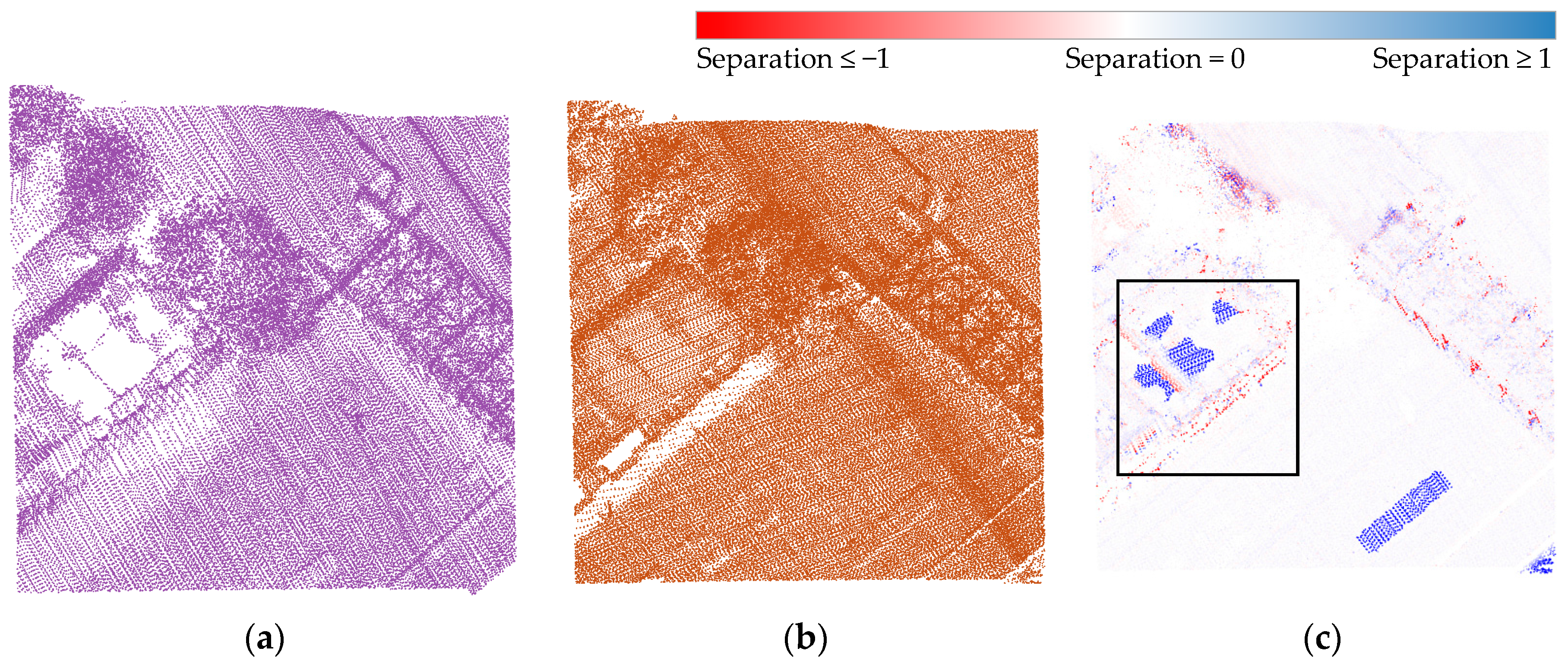
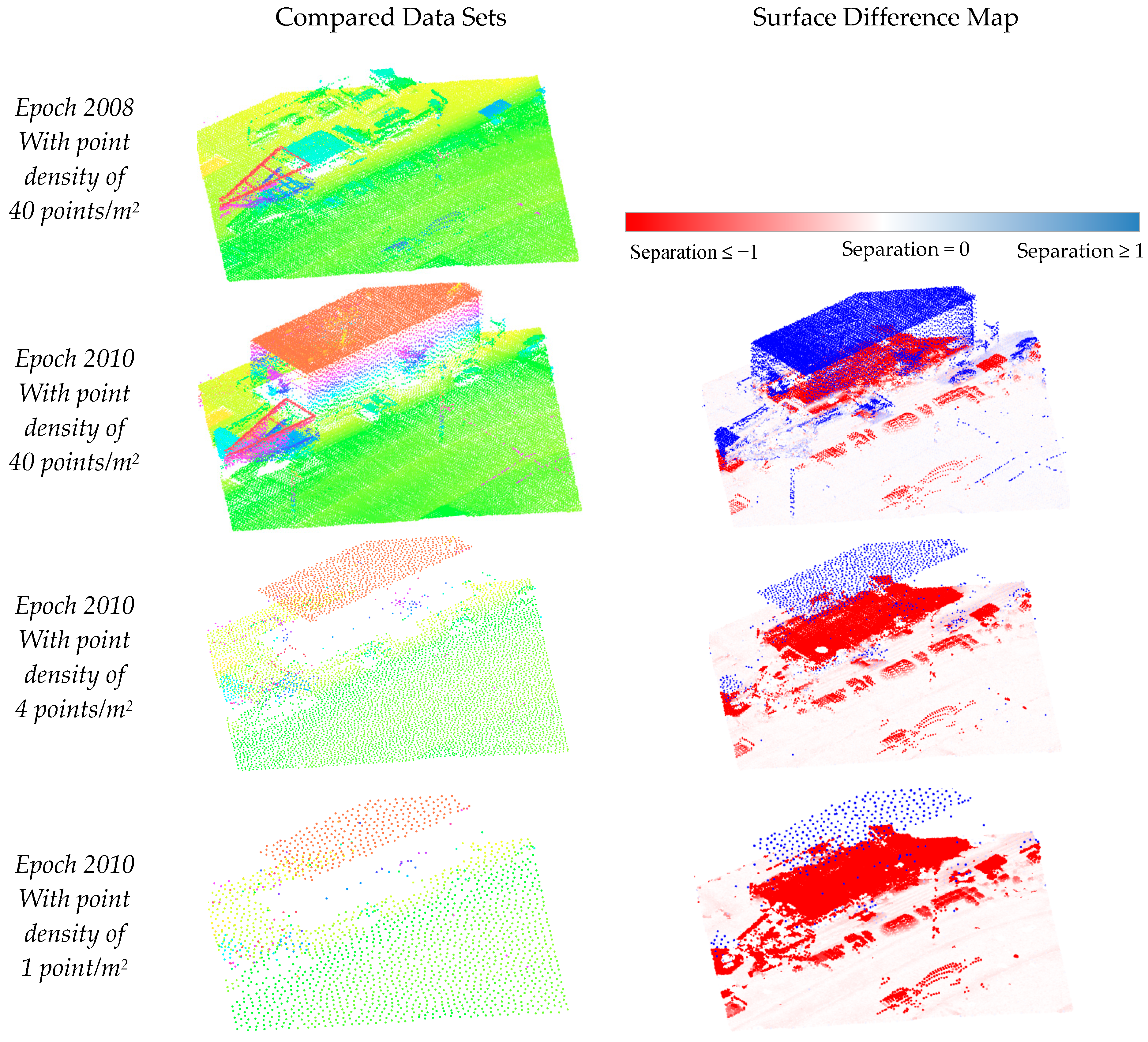
For every point in one epoch of data, we search within its 1.0 m (radius) 3D neighborhood to check whether there is a point from the other epoch. If there are no points from the other epoch, this implies a difference greater than 1.0 m. In these cases we record a difference value >1.0 m. If there are points from the other epoch of data, we define the surface difference as the distance from the selected point to the nearest fitted plane in the point cloud of the other epoch.
A 3D neighborhood of 1.0 m radius points is chosen because the point density is greater than 1 point/m
2 in most locations of our dataset. This ensures that the comparison is not affected by the point density. Although we have two data sets that have similar point densities, in order to make sure that a 1.0 m neighborhood is suitable for comparisons between data sets with different point densities. We simulated several data sets with our test data by reducing the point density of one of the epochs (see
Figure 1).
Figure 1.
Examples of the surface difference map for various point densities. Comparison of data sets with different densities from the year 2010 with the data from the year 2008 showed that the locations of the changes are the same in all the difference maps. This indicates that the surface difference map generated with a neighborhood of 1.0 m points is suitable for all the data sets that have a point density larger than 1 point/m2.
The difference map contains the geometric indication of whether there is a change or not. However, not every difference is a change (
Figure 2), and sometimes part of a change is not represented as a large value in the difference map (
Figure 3).
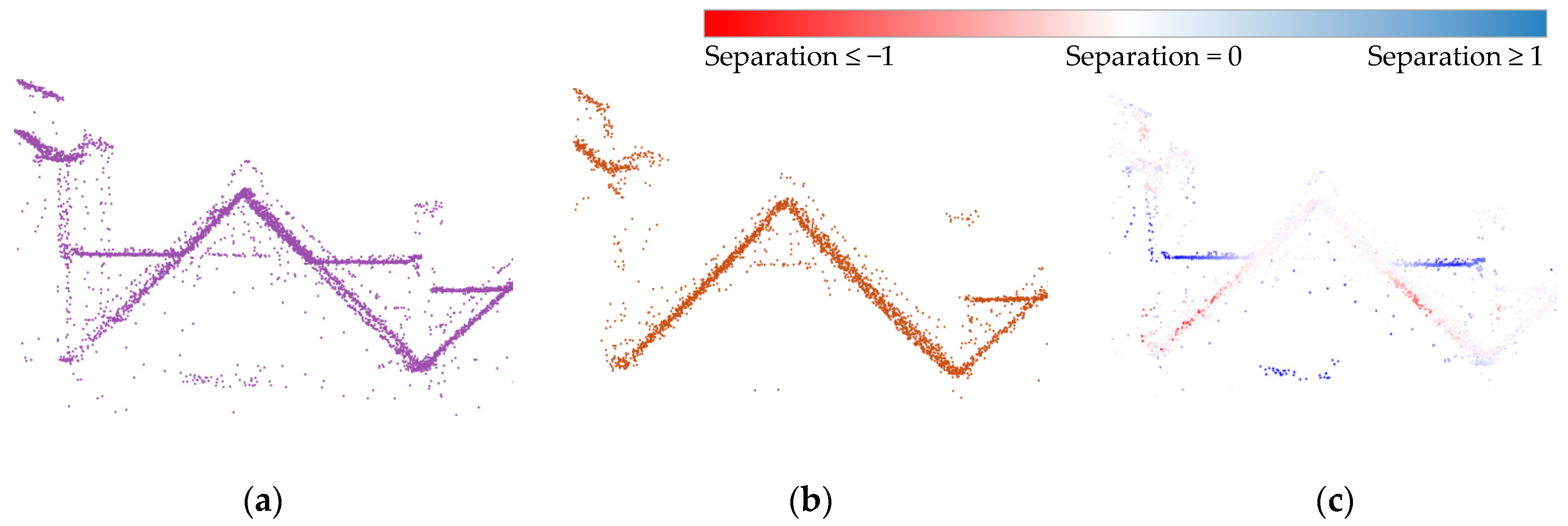
Figure 2c shows the difference map containing several points with a surface difference greater than 10 cm. However, these differences are caused by lack of data in the other epoch and therefore cannot be considered as a change in an object. Conversely, points with a difference value less than 10 cm may belong to a changed object.
Figure 3 is an example that displays points with a surface difference of less than 10 cm in the connections between a dormer and a roof; the change was detected because the dormer was newly built.
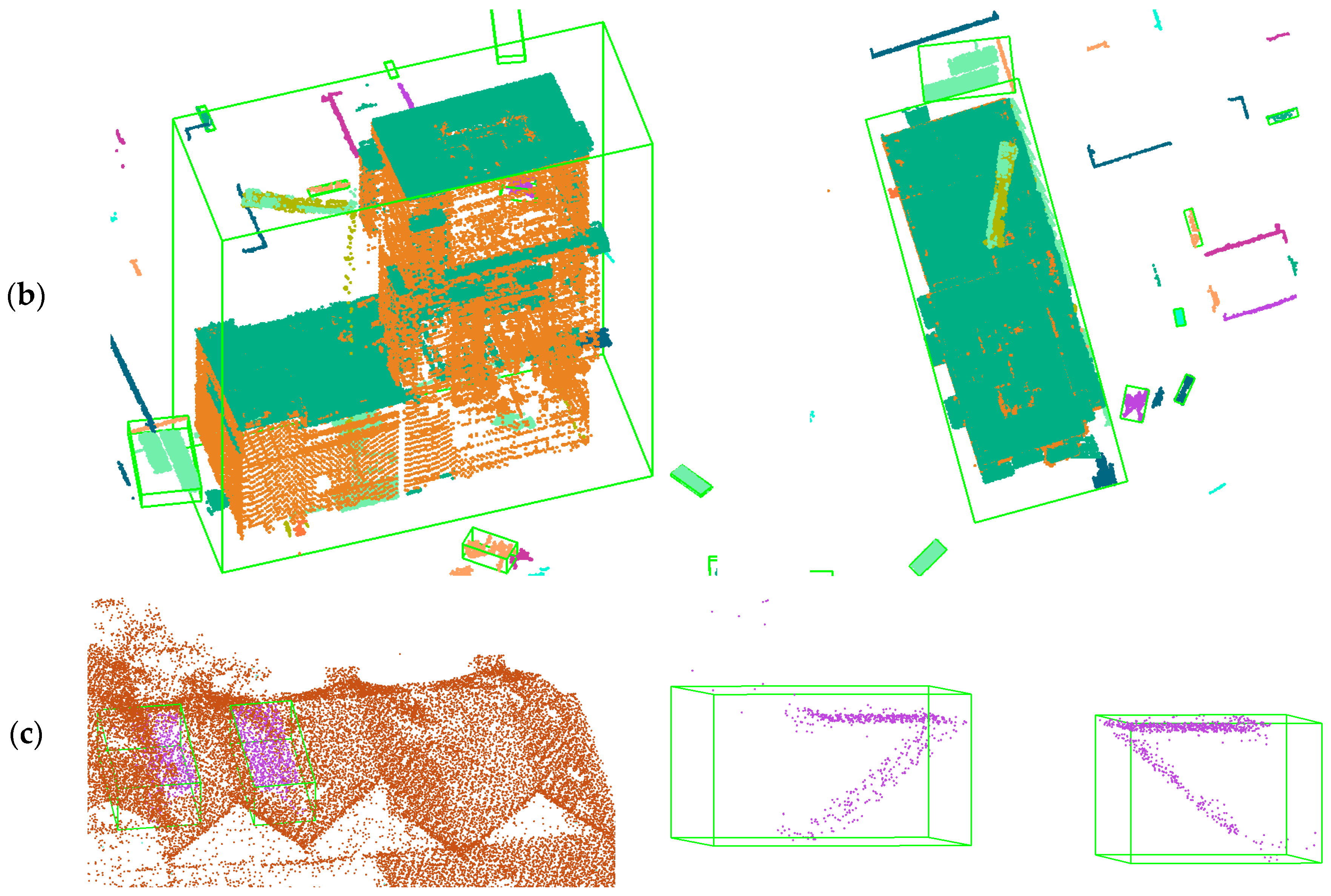
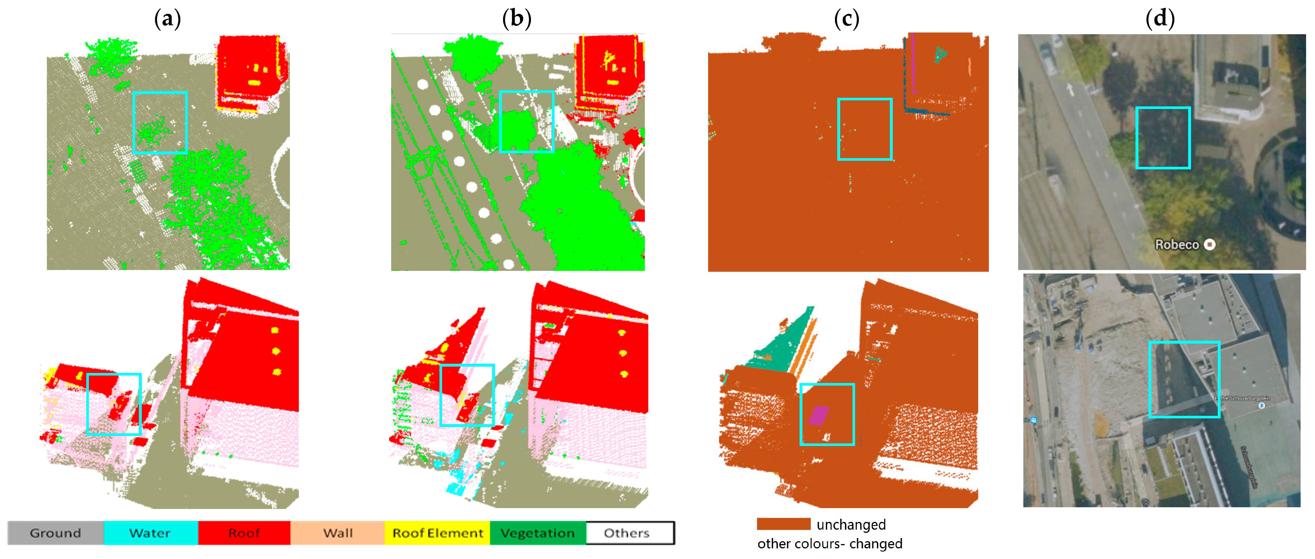
Figure 2.
(a,b): Different colors represent different epochs of data, (a) 2008, (b) 2010; (c) Surface difference map derived from the two epochs. Points with a great difference do not always denote a change. For example, in (c) blue points in the rectangle are unknown points because there is no data for the roof in thr 2008 epoch data (perhaps caused by water on the roof), although they have high difference values.
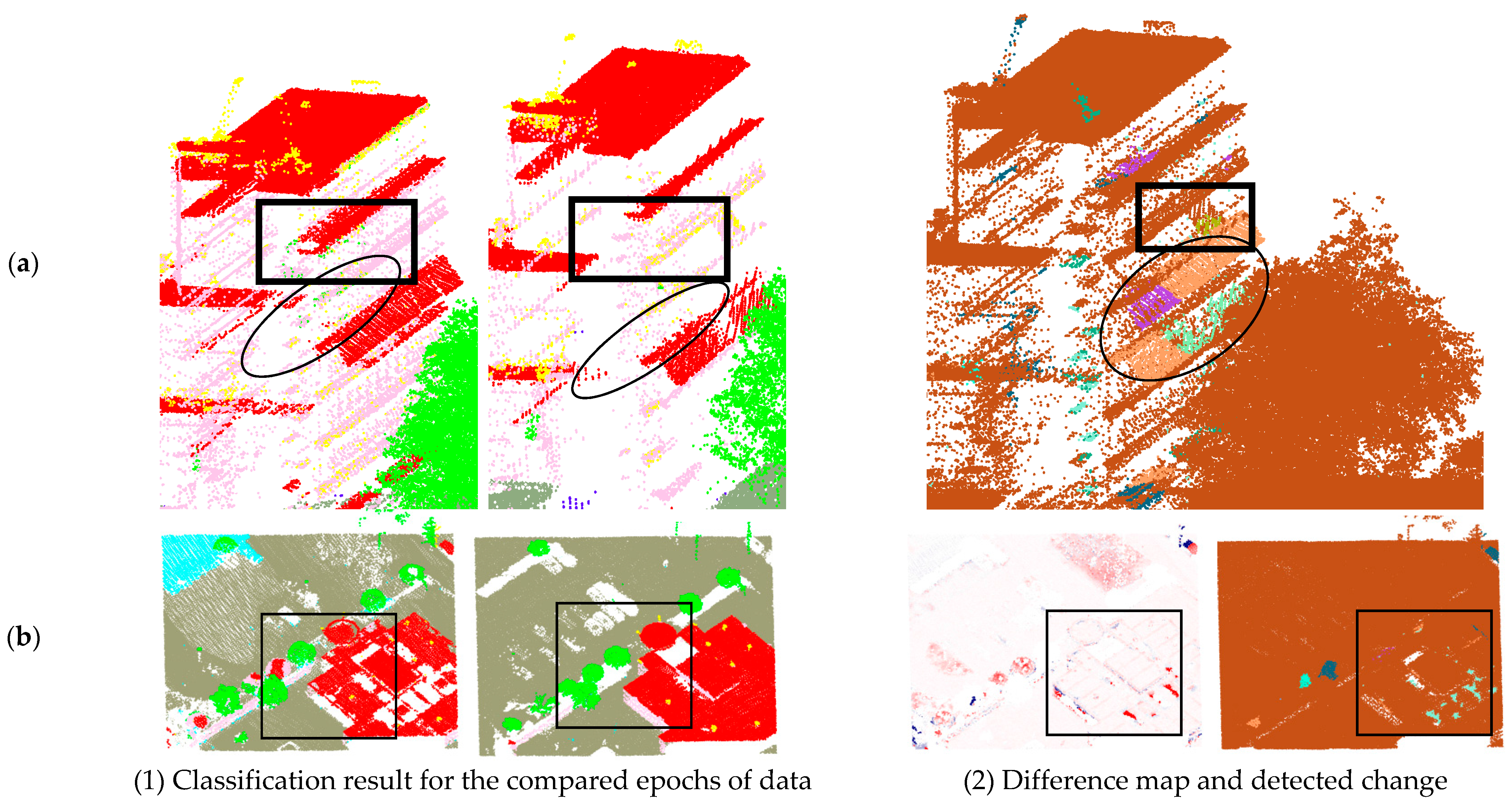
Figure 3.
(a,b) Different colors represent different epochs of data, (a) 2012, (b) 2010; (c) Surface difference map—both epochs merged. The points in the rectangle have a distance difference ≤0.08 m, although there is indeed a change. The difference value is small because the points on the roof from the other epoch are in the neighborhood of the points on the dormer and they are quite close to each other. The problem is to identify the areas in the rectangle as being changed when the difference value is low.
Our task is to assign the labels of “changed”, “unchanged”, and “unknown” to each point according to the surface difference map.
3.2. Detecting a Change
The strategy for interpretation of the surface difference map is as follows: points classified as building (wall, roof, or roof element) in the scene classification are selected. All building points are assumed to be unchanged except for those distinguished as “unknown” or “changed”.
Points with a difference value greater than 1 m in one epoch for which, even in a two dimensional neighborhood, no nearby points can be found in the other epoch are considered “unknown” (see
Figure 4) . This occurs in areas where there is a lack of data in one epoch because of occlusions or pulse absorption by the surface. For walls, large surface difference values may occur. However, our algorithm will label the points for the wall as “unknown” instead of “changed” if there has been no change to the roof of that same building. Due to a lack of evidence as to what happened with the wall, the points are labelled as “unknown”.
Figure 4.
Points labelled as “unknown” for walls. (a) a wall scanned with dense points; (b) the same wall scanned with sparse or (c) no points in another epoch.
Figure 4.
Points labelled as “unknown” for walls. (a) a wall scanned with dense points; (b) the same wall scanned with sparse or (c) no points in another epoch.
In
Table 1, the “seed neighborhood radius” and the “growing radius” indicate the maximum radius for allowing a point participating in the seed plane extraction and the plane growing phase. The “minimum number of seed points” means the minimum number of points that are required for initialization of a plane. The plane parameters are obtained from the Hough space and 10 points are required as the minimum number of seed points to ensure a reliable plane extraction. The “maximum distance of a point to the plane” ensures that only nearly co-planar points are added to the seed plane. The 1.0 m radius is set to ensure that the surface can be extended with neighbouring points on the same surface. This setting needs to be adjusted for processing datasets with a different point density.
Table 1.
Parameters for the surface growing and connected component algorithm.
Table 1.
Parameters for the surface growing and connected component algorithm.
| Surface Growing | Connected Component |
|---|
| Parameters for seed selection | Parameters for growing | Maximum distance of component |
| Seed neighborhood radius | 1.0 m | Growing radius | 1.0 m | 1.0 m |
| Minimum number of seed points | 10 pts | Maximum distance of a point to the plane | 0.1 m |
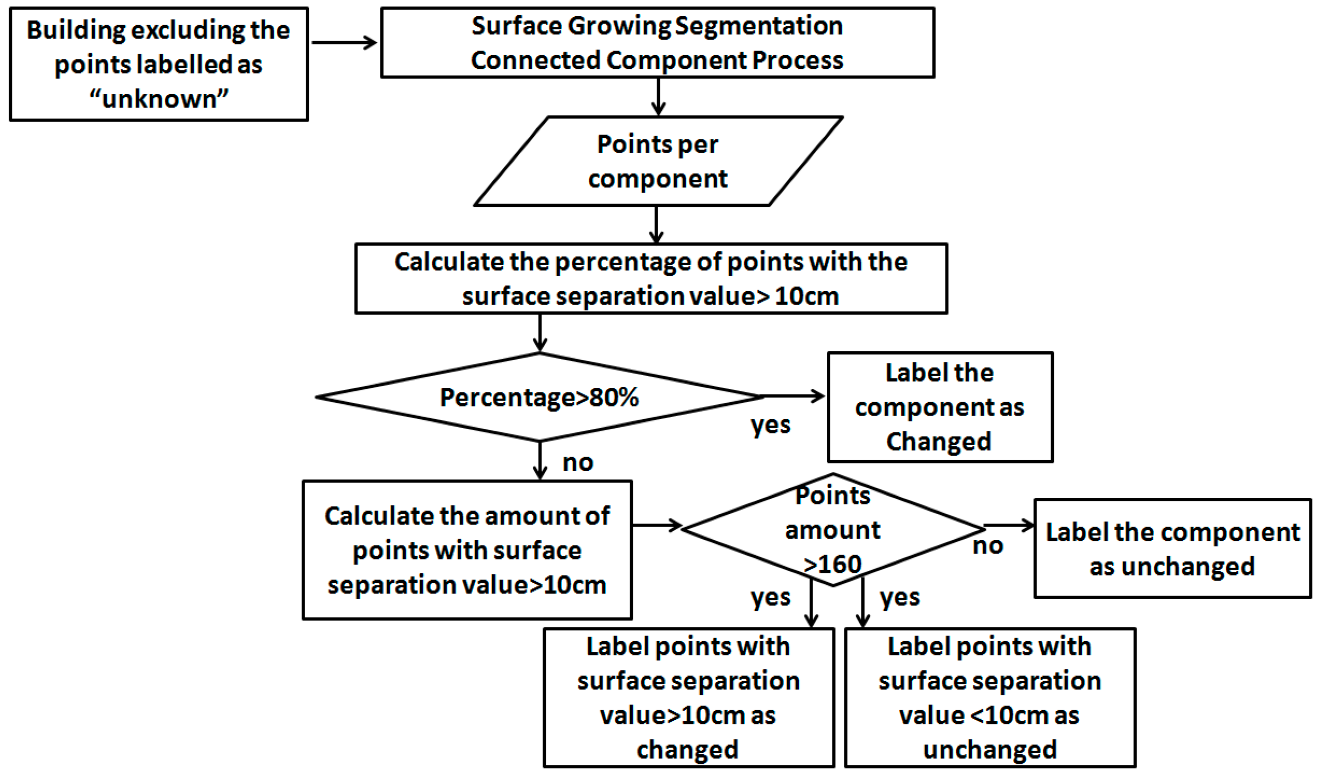
Generally, “changed” points have a high difference value, although they cannot be selected using a simple threshold in the difference map. Therefore, we derived a rule-based decision-tree to detect “changed” points in surface difference maps. The decision-tree is shown in
Figure 5. The “unknown” points are first excluded from the data sets. The remaining points are grouped into planar segments using the surface growing method [
24]. Within each segment, points are further separated into connected components with a smaller radius than during the planar surface growing step. This separates two nearby objects that are located in same plane. For example,
Figure 6a shows two dormers belonging to the same planar segment, and after deriving connected components, they are separated into two components. These components are used as the basic units for identifying changed points. Parameters used in the surface growing and connected component algorithms are listed in
Table 1.
If, for each connected component, the vast majority of points have surface differences greater than the maximum strip difference, the whole component is very likely to be a change and will be labelled as “changed”. Otherwise, the component may be unchanged or only partly changed. If partly changed, the changed part is only labeled as “changed” by checking its area. The parameters for the vast majority, the maximum strip difference, and the area are listed in
Table 2 and the reason for the parameter setting is given.
Figure 5.
Identification of changed and unchanged points using a decision-tree.
Figure 5.
Identification of changed and unchanged points using a decision-tree.
Figure 6.
(a) The two dormers in the red rectangle belong to the same planar segment and therefore need connected components analysis to separate them (different colors indicate different segments); (b) Both changes to roofs and dormers are detected (two data epochs are merged).
Figure 6.
(a) The two dormers in the red rectangle belong to the same planar segment and therefore need connected components analysis to separate them (different colors indicate different segments); (b) Both changes to roofs and dormers are detected (two data epochs are merged).
Table 2.
Parameters for deciding on change.
Table 2.
Parameters for deciding on change.
| Name | Thresholds | Reason for the Choice of Thresholds | Suitability to Transfer to Other Datasets |
|---|
| Vast majority | 80% | Tested | To be adjusted according to the training data. |
| Maximum strip height difference between two epochs of data | 10 cm | Registration error in each epoch was shown to be below 5 cm. | To be adjusted to the maximum registration error. |
| Area | 160 points (4 m2) | The average point density is 40 pts/m2 , and all buildings larger than 4 m2 should be mapped. | To be adjusted to the point density and the definition of relevant change. |
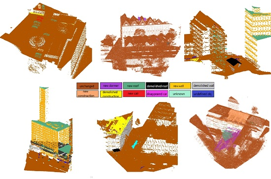
3.3. Classification of Building Change
Points detected as changes in a building are extracted and a second classification step is performed on these changes. This second classification step is required to understand the activities that could have possibly led to the changes detected for a building. For example, by identifying changes to roof elements on top of a building (
Figure 7a), we can infer that these elements may be cars, and that there is a parking lot on top of the building.
Figure 7.
Connected components of changed objects are classified based on their context. (a) 2008 vs. 2010; (b) 2010 vs. 2012.
Figure 7.
Connected components of changed objects are classified based on their context. (a) 2008 vs. 2010; (b) 2010 vs. 2012.
There are various types of objects that may be present on building roofs or attached to walls. Most changes to walls are caused by sun shades (which are open in one epoch but closed in the other epoch), stairs, flags, or vegetation near walls. Compared to the changes to roofs (e.g., a new dormer or the addition of a floor), changes near walls are less likely to be related to construction activities. For this reason, the second classification step is performed only for changes concerning roofs and roof elements.
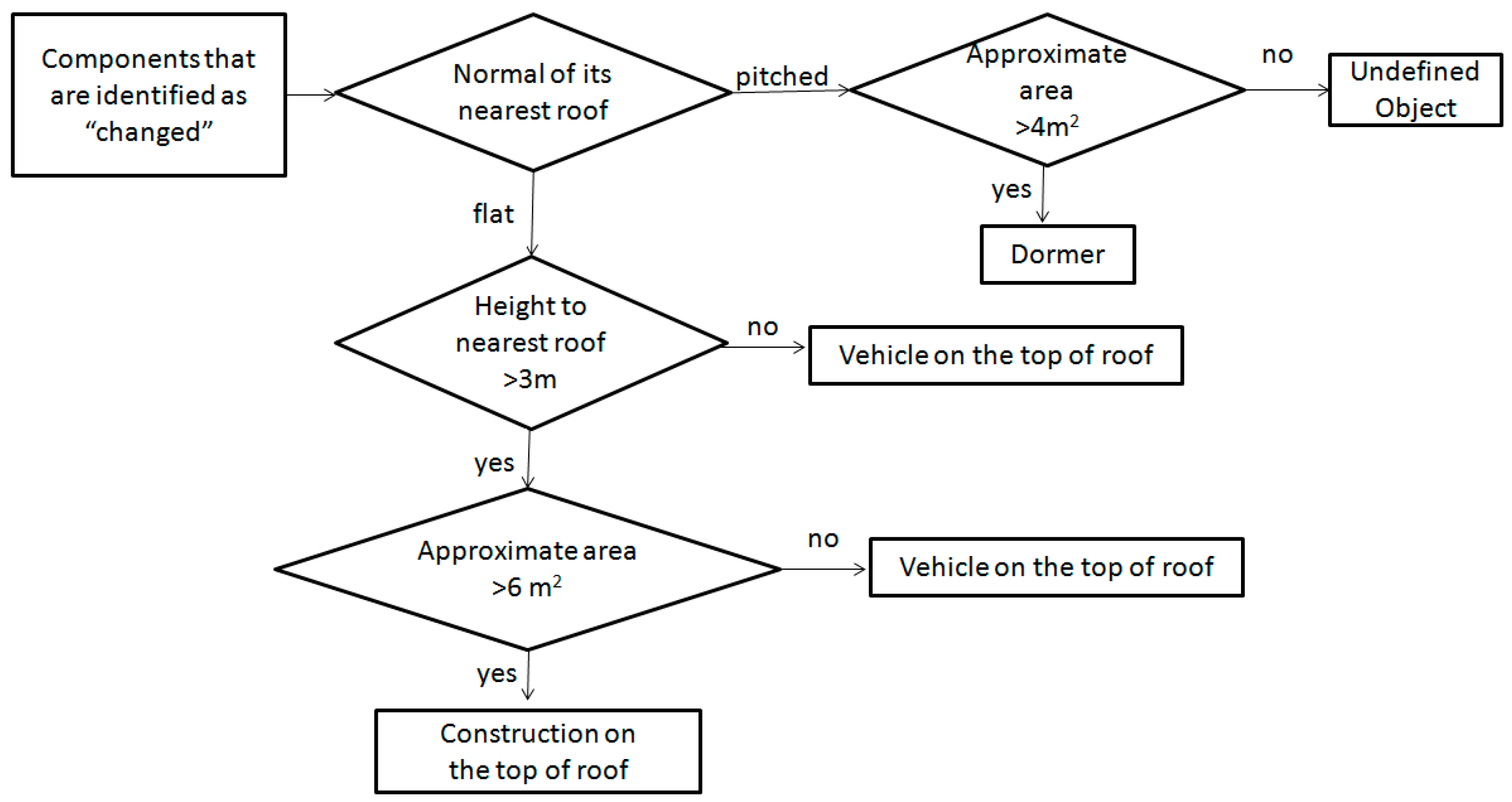
Based on the size of changes and the underlying building structure, changes on a roof top are classified as dormers, cars or “other constructions”. The difference between a dormer and “other constructions” above the roof line is that the latter involves relatively large changes compared to a dormer. The attributes used for the classification are area, height to the nearest roof, the normal vector direction of the nearest roof (which indicates a pitched or a flat roof) and the labels from the scene classification results.
Rules are defined to classify these components. Large areas of points labelled as changed indicate a change to a roof. Small changes occurring on a pitched roof are more likely to be newly built or removed dormers or chimneys. If changes occur on a flat roof, they are probably constructions above the roof line or cars. These rules are used in a decision-tree, and have been established as a rule-based classifier with some defined values according to the knowledge (see
Figure 8). All defined values are based on the authors’ knowledge and are explained in
Table 3.
Figure 8.
Rule-based classification of changes.
Figure 8.
Rule-based classification of changes.
Table 3.
Defined parameter values for the rule based classifier.
Table 3.
Defined parameter values for the rule based classifier.
| Attribute Name | Value | Explanation |
|---|
| Approximate area | | |
| On pitched roof | On flat roof | 4 m2 | 6 m2 | Minimum area of interest | Area of small vehicle |
| Height to the nearest roof | 3 m | The maximum height of a car |
| Class label of point in the scene classification | “roof”/”roof element”/“wall” | For understanding the context |
3.4. Analysis of Changed Building Objects
After the points are identified as “changed” and classified, the results are points organized as connected components. These components have not been identified as building objects yet, and they may represent only a small part of an object. How points are organized as building objects and how the changed objects are analyzed is described in the following subsections.
3.4.1. Changed Building Objects
The points that are identified as changed can be organized into building objects once we have labelled all the points with: (1) the type of object class from the change classification; (2) the labels “changed”, “unchanged”, or “unknown”; and (3) the signs from a difference map indicating a newly built or demolished structure. We distinguish buildings as being entirely changed or partly changed.
If there is a change to the roof of a building, all points that group together in a 2D connected component step will be labelled as an entirely changed building. If changes are made to building elements, the local 3D connected points will be only labelled as partly changed.
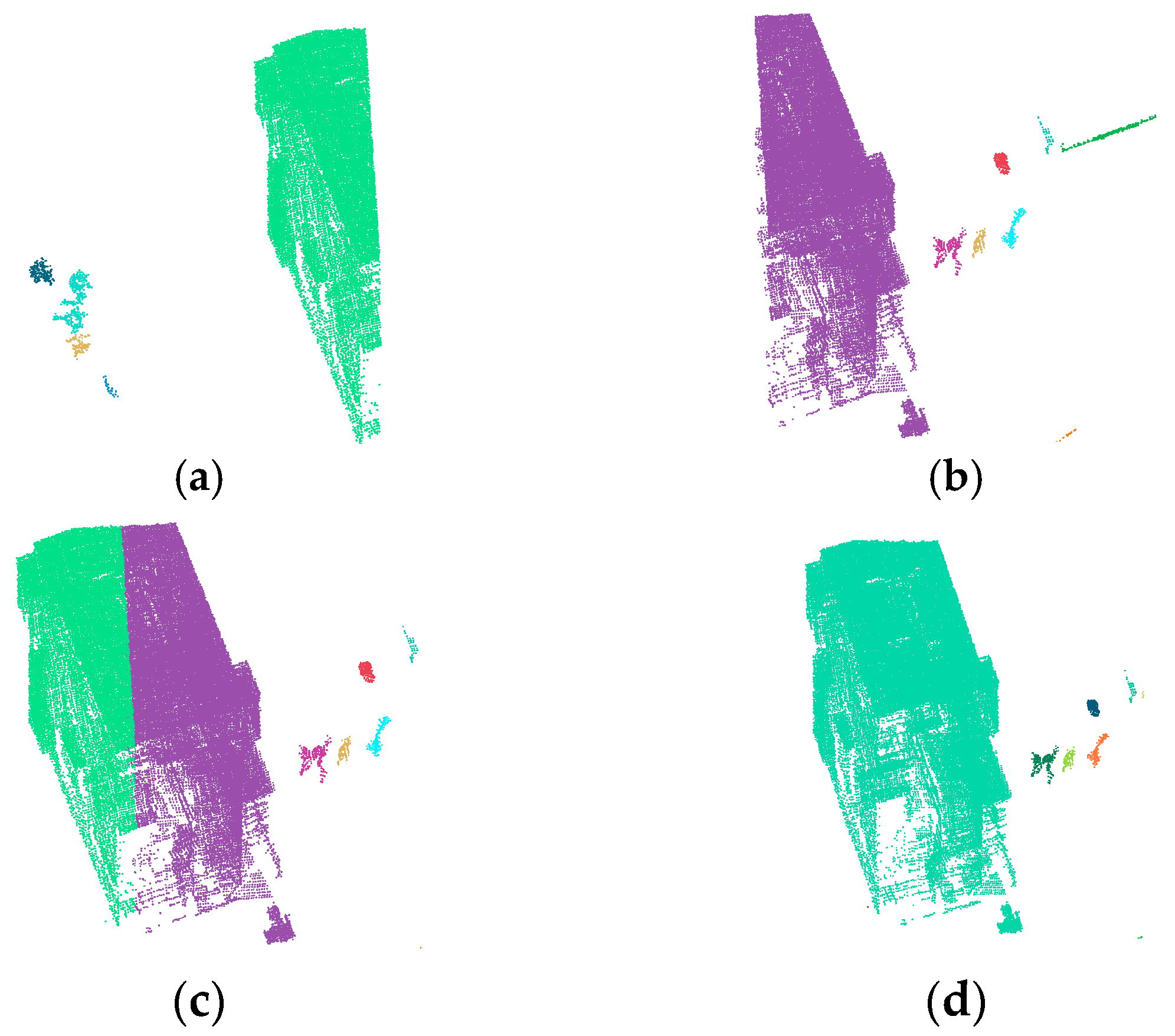
3.4.2. Merging Objects at Tile Boundaries
So far, changes are detected within tiles of, for example, 50 m × 50 m. Typically, buildings are stored in different tiles, as shown in
Figure 9a–c. As changed objects may occur on tile boundaries, a merging step is needed to detect a single object instead of two (
i.e., one in each neighbouring tile). To solve this problem, adjacent components are merged across tile boundaries, as described by Vosselman [
25].
Figure 9d shows the components after they have been merged.
Figure 9.
Objects are cut and stored in different tiles (a) and (b) during the processing of large data sets. Components have been merged in (c) and (d). (a) building part in one tile; (b) building part in another tile; (c) the same building part belonging to different objects; (d) the same building part merged into the same object.
When building objects have been formed, minimum 3D bounding boxes are calculated for these objects. Their width, length, height, area, volume, and location of their center point are determined from their 3D bounding boxes.
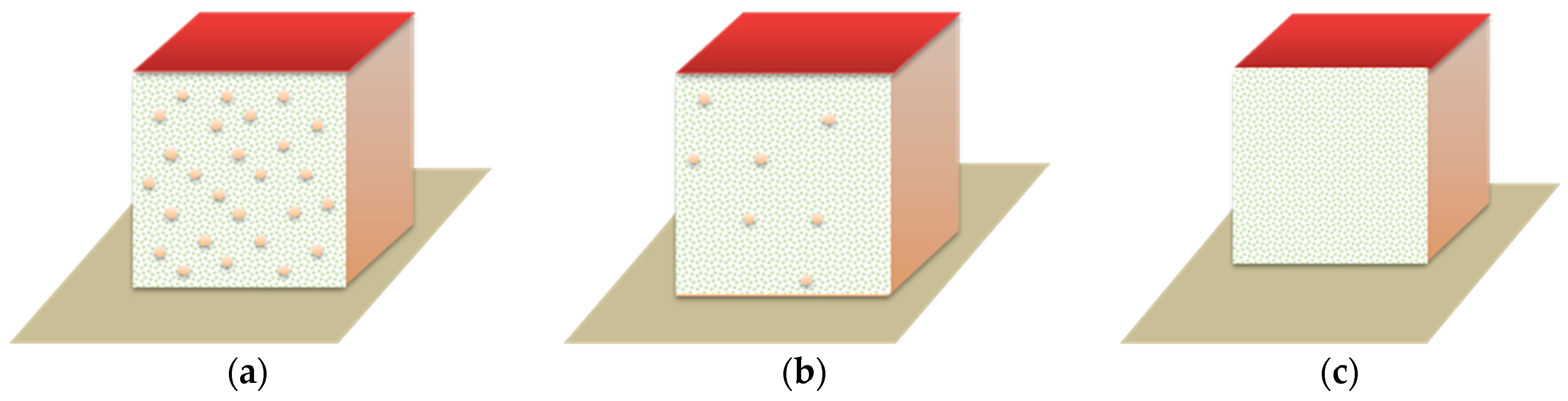
Among all the changes near buildings we found, there are some that are irrelevant for the municipality. Common examples are changes to extensive areas of flowers and shrubs, to fences, and railings in gardens on rooftops of buildings. Bounding boxes have been used to measure more precisely the size of a change. This measure of size is used to separate irrelevant changes (<4 m2) from relevant ones. For changes <4 m2 and a “length: width” ratio greater than 10, no 3D bounding boxes are calculated.
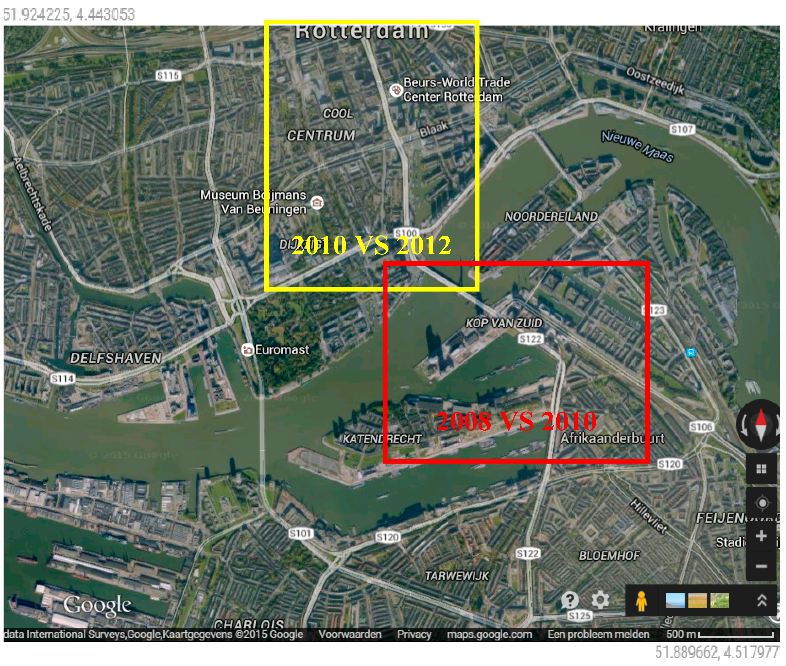
4. Data Sets
The research we present here originated from a request from the Municipality of Rotterdam (the Netherlands) to help in monitoring changes to buildings using ALS data. Three data sets, located in commercial and residential areas of Rotterdam, have been used. The data of the commercial area was scanned in years 2008 and 2010; data sets of the residential area were acquired in years 2010 and 2012 (
Figure 10). The point densities for the data sets 2008, 2010, and 2012 are average 30 points/m
2, 35 points/m
2 and 40 points/m
2, respectively. The strip difference within an epoch and between different epochs had a maximum value of 10 cm. As the data sets already register well (with a strip difference less than 10 cm), no extra steps for registration were required. All data sets underwent scene classification and were then divided into tiles of 50 m × 50 m.
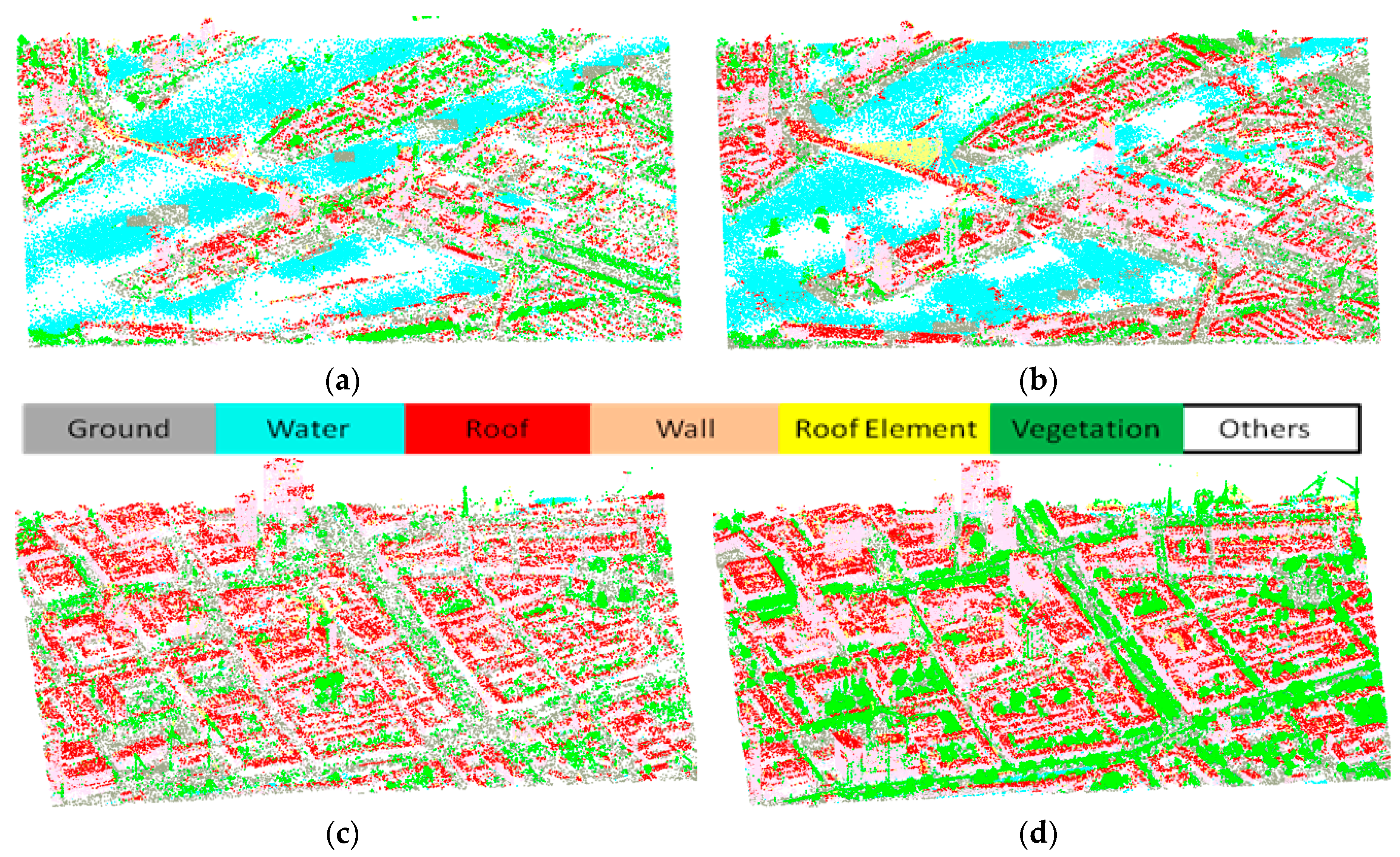
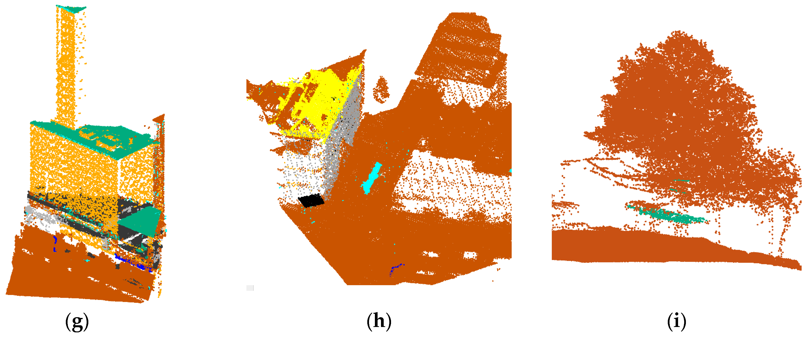
Figure 11 shows four examples of the result from the scene classification step. Bridges and its cables are classified as building roof and roof elements in data set 2008 and 2010. Data set 2010 was obtained in the fall and the 2012 dataset was obtained in the fall. Therefore, tree points are more dense in the 2012 data set.
Figure 10.
Locations of test areas and their data sets. (From Google earth and the coordinates are approximately measured from the map).
Figure 10.
Locations of test areas and their data sets. (From Google earth and the coordinates are approximately measured from the map).
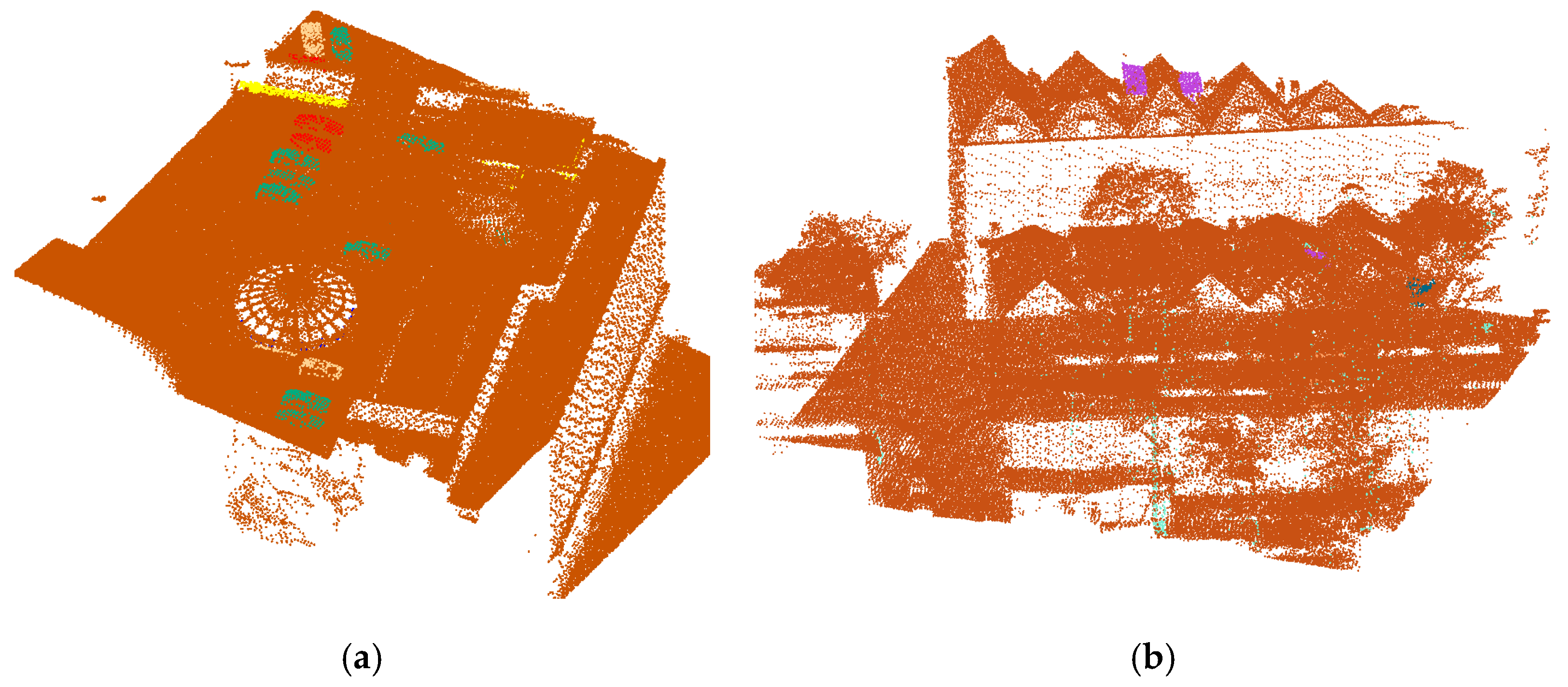
Figure 11.
The scene classification results for the test areas. (a) 2008—commercial area; (b) 2010—commercial area; (c) 2010—residential area; (d) 2012—residential area.
Figure 11.
The scene classification results for the test areas. (a) 2008—commercial area; (b) 2010—commercial area; (c) 2010—residential area; (d) 2012—residential area.
5. Result and Discussion
Our change detection procedure comprises change detection, classification of any change detected, and object-based analysis. This procedure includes generation of surface difference maps and change identification. The results for each step in the procedure are described below. As the compared data sets are merged into one with different epoch numbers, all the results will be shown in a merged version.
5.1. Detecting Change
Results of the change detection step are shown and the causes of errors in detecting change to buildings are discussed here. The true positives (TP), false positives (FP), and false negatives (FN) are counted “per change” by three people after visual inspection of the compared data sets, the corresponding surface difference map, and our change detection results on a computer screen. To provide some context, an area with 10 m × 10 m around the detected change is shown, together with a high resolution aerial image of the area. The experts indicate whether the detected change is a change to a relevant object. The difference map is also used to verify whether all geometric differences resulted in a detected change. If it is a relevant changed object and we detected it correctly in our result, the change is counted as true positive. If we found a changed object in our result but three experts considered it not a change, the change is a false negative, and if the experts found some changes that we did not detect in the result, the change is a false positive. The completeness and correctness are calculated with the following equations:
It is notable that one large building change is counted as one change, the same as a small change, regardless of the number of points within the change. In order to know how the scene classification result affects the change detection result, we also calculated the percentage of errors that are caused by the scene classification result.
5.1.1. Surface Difference Mapping
A surface difference map is generated from original data sets, regardless of the scene classification results. Some difference maps have already been shown in
Figure 1 (
Section 3.1) and, as discussed, the point density does not affect the surface difference map. More difference maps can be seen in
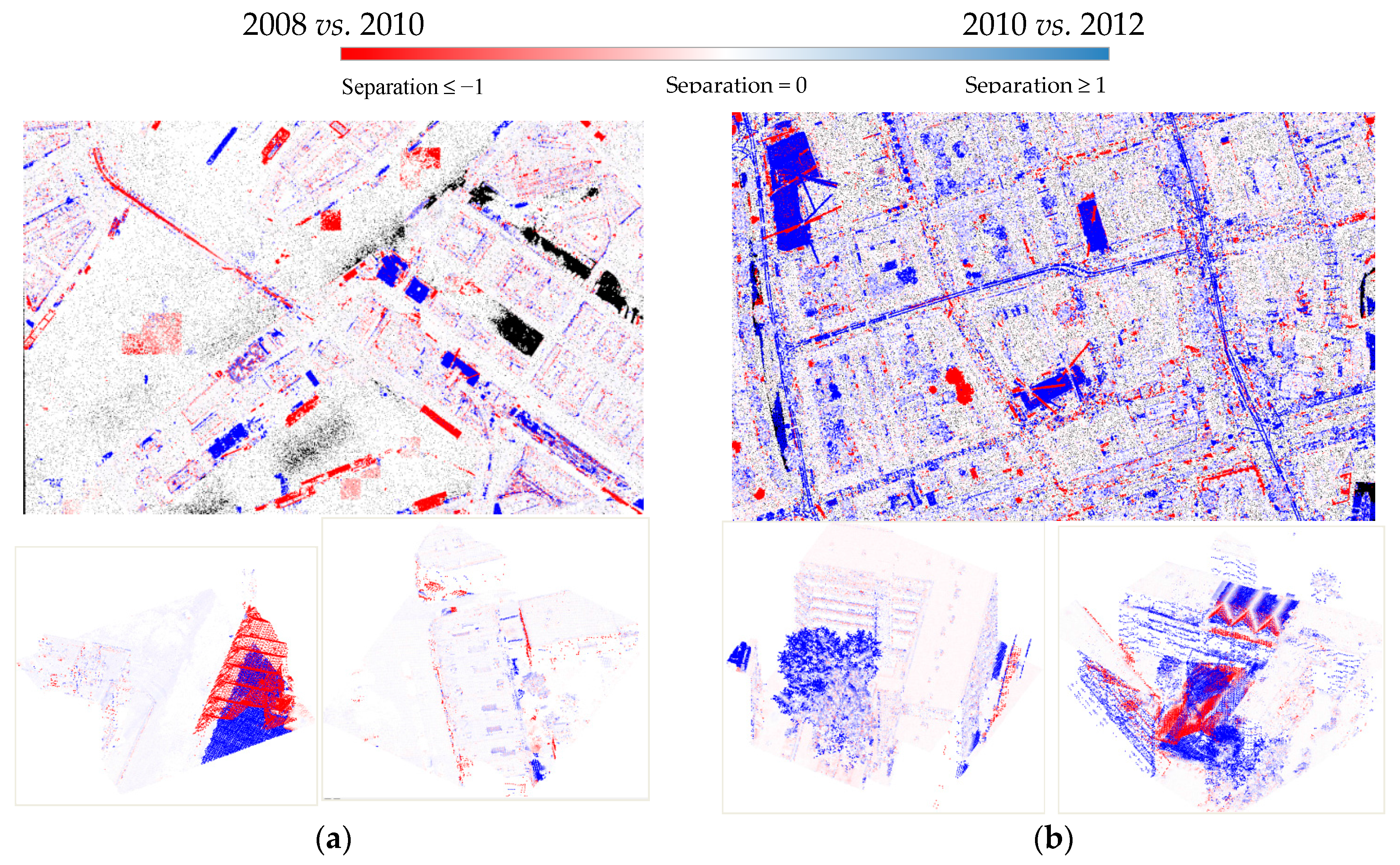
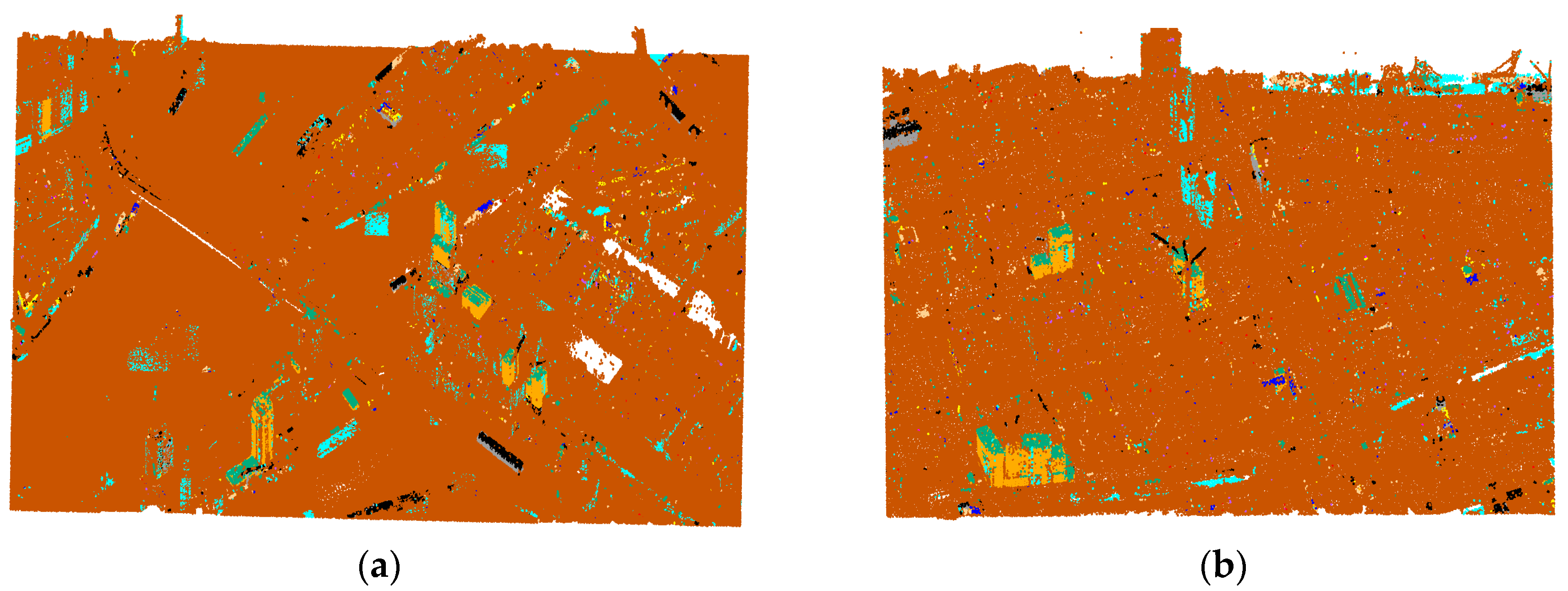
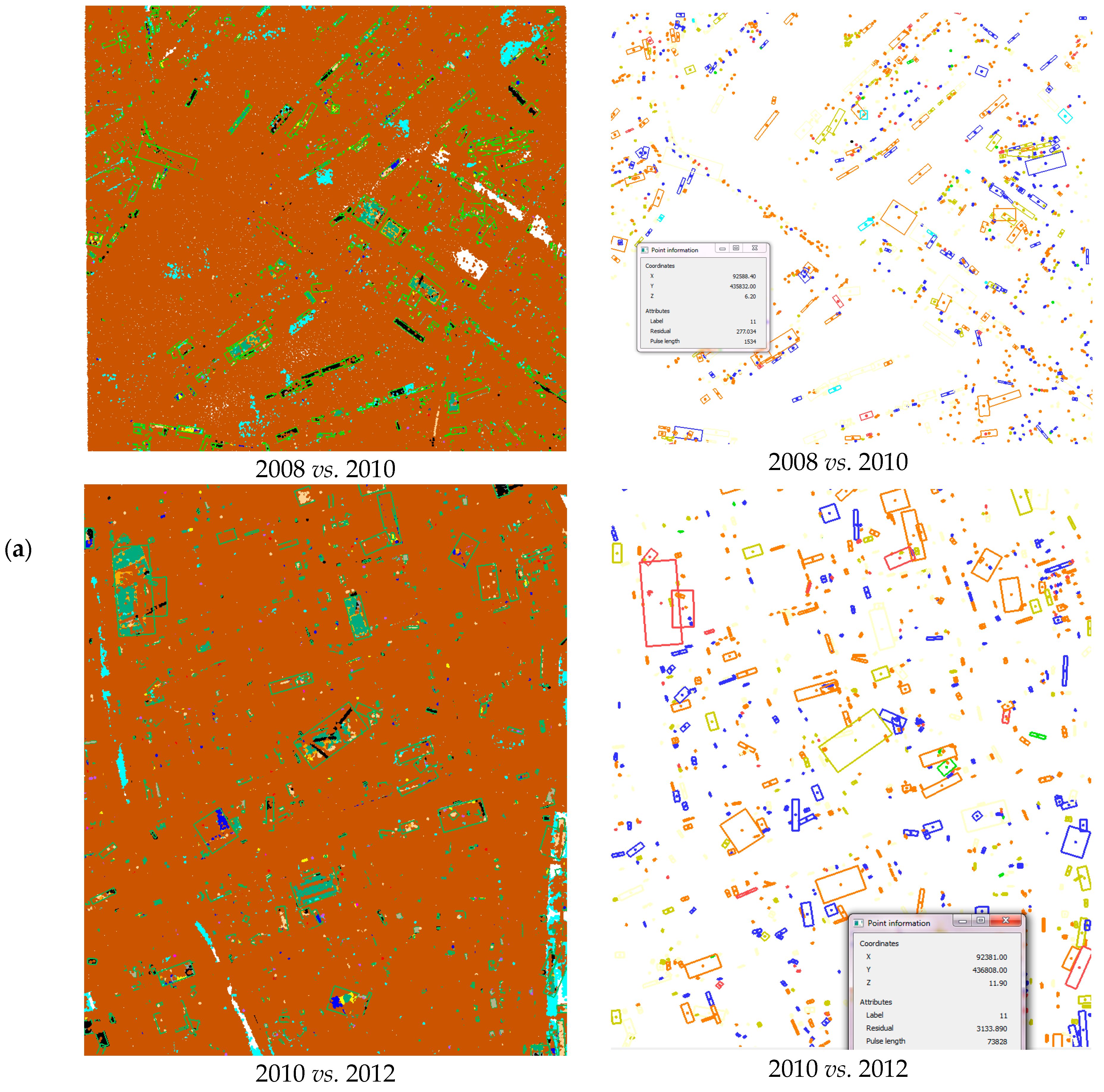
Figure 12. The surface difference map gives only clues as to where changes may have occurred in the data sets. To improve their display, all the data sets have been merged into one. Different colors show different values of the differences between the compared data sets.
Figure 12.
Surface difference maps for (a) 2008 vs. 2010 and (b) 2010 vs. 2012. Maps in the first column are the overall visualization of the test area, and maps in the second column are detailed visualization from some tiles.
Figure 12.
Surface difference maps for (a) 2008 vs. 2010 and (b) 2010 vs. 2012. Maps in the first column are the overall visualization of the test area, and maps in the second column are detailed visualization from some tiles.
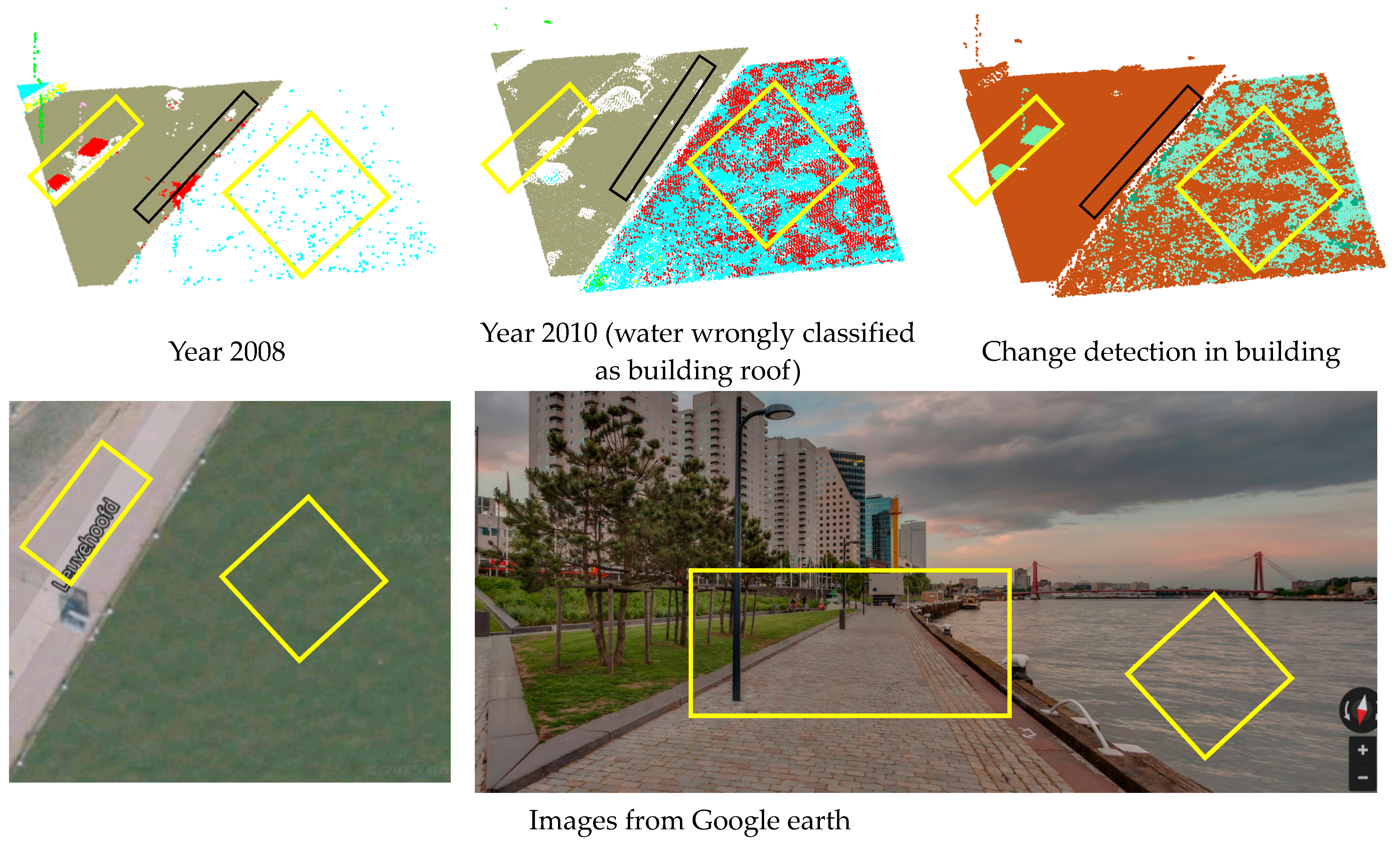
In
Figure 12, significant differences can be directly observed on the surface difference maps where the colors become deeper. Red points appearing in the middle of water in
Figure 12a indicate large differences in water surfaces. This large difference is caused by lack of points on the water in one of the epochs, while points were recorded in the other epoch. These difference maps are the inputs for the change identification step.
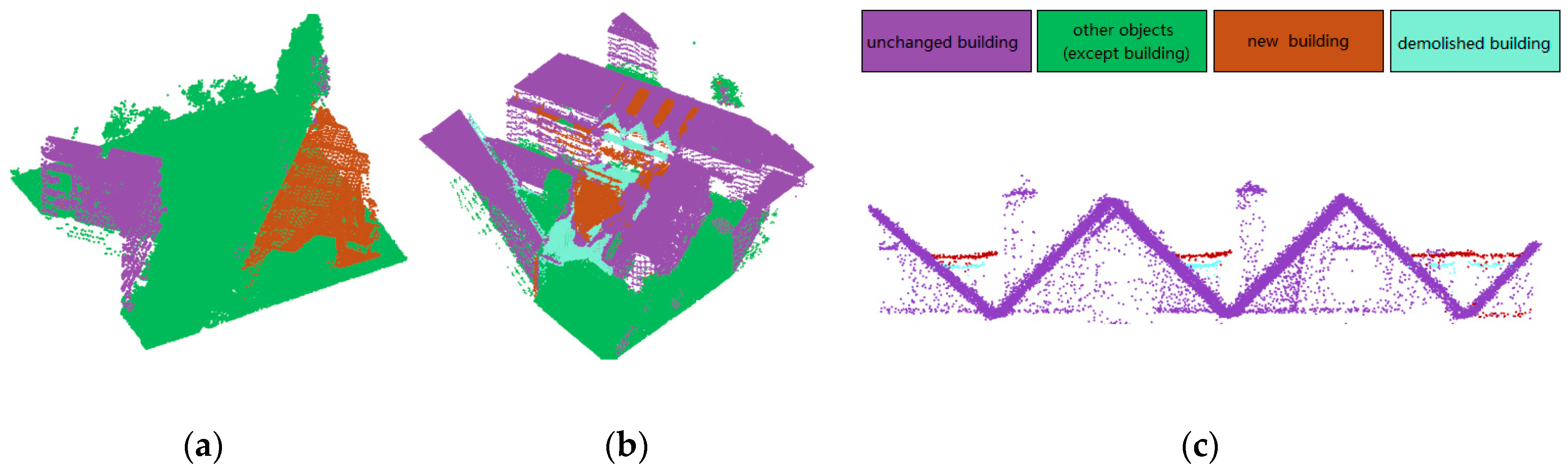
5.1.2. Change Detection Results
Using the surface difference map, we labelled the data sets as “changed”, “unchanged”, and “unknown”.
Figure 13 shows some results of both types of change (an entire building change (a), as well as changes to building elements, e.g., changes (b) and (c)). The interpretations “demolished” and “new” can be decided from the sign of the surface difference value in the difference map. For example, the points seen in epoch 2008 but not in epoch 2010, are “demolished” objects. A small change is shown horizontally for clearer visualization in
Figure 13c. As there are new points in epoch 2010, as well as demolished points beneath them in epoch 2008, we can infer that there are some extensions of the objects. To understand which objects caused the extension, the changes need to be classified.
Figure 13.
(a,b) Examples of large changes in buildings; (c) changes to dormer sizes in the merged data sets (removed dormers and extensions to dormers in height and length).
Figure 13.
(a,b) Examples of large changes in buildings; (c) changes to dormer sizes in the merged data sets (removed dormers and extensions to dormers in height and length).
We selected 20 tiles with changes randomly from each test area to evaluate the performance of the change detection method. There are more false positives than false negatives, so completeness is greater than accuracy,
i.e., 50% (
Table 4) of identified changes are not relevant. However, the vast majority of changes to buildings are actually detected, making it convenient to only look at the detected changes and ignore the irrelevant ones.
Table 4.
The completeness and correctness of detected change.
Table 4.
The completeness and correctness of detected change.
| | True Positive | False Positive | False Negative | Correctness | Completeness |
|---|
| 2008 vs. 2010 | 34 | 34 | 3 | 50.00% | 91.89% |
| 2010 vs. 2012 | 35 | 30 | 6 | 53.86% | 83.33% |
As shown in
Table 5, 40% of the errors (false positives and negatives) are due to incorrect scene classification in Test area 1, and 67% in Test area 2. In Test area 1, which is a commercial area of Rotterdam, the main propagation errors from scene classification are large and long balconies in walls, which are incorrectly classified as roofs. In Test area 2, a residential area, the error propagation mainly arose from trees that are so dense that they were wrongly classified as building roofs. So, changes in trees were incorrectly detected as changed building objects.
Table 5.
Percentage of errors due to scene classification and errors due to the method of change detection used.
Table 5.
Percentage of errors due to scene classification and errors due to the method of change detection used.
| | False Positive | False Negative | |
|---|
| 2008 vs. 2010 (Test area 1) | 34 | 14 | 3 | 1 | Errors due to the scene classification error
40% |
| 20 | 2 | Errors due to limitations of the change detection method
60% |
| 2010 vs. 2012 (Test area 2) | 30 | 18 | 6 | 6 | Errors due to the scene classification error
67% |
| 12 | 0 | Errors due to limitations of the change detection method
33% |
Note that in
Table 5 there are two false negatives (relevant changes that are not detected) due to our method in Test area 1. These two relevant changes are detected in the change detection method, but the 3D bounding boxes are not generated. The reason for this is that we applied a threshold value for the ratio of the length to width to exclude some thin and long objects such as fences and railings during the change quantification stage. These two relevant changes were roofs that are long and narrow, so 3D bounding boxes were not generated for them.
The advantage of using raw lidar data, instead of using DSM or image, is that lidar data can penetrate trees and the information under trees can be preserved. If a change happens under trees, DSM or image may not detect the change. One such case is shown in figure (i) in
Section 5.2.1.
5.1.3. Change Detection Error Due to Scene Classification Error
The points on the surface difference map that are labelled as part of a building are selected for the building change-detection step. When buildings are not correctly classified in the scene classification in any one of the epochs, it will influence the quality of building change detection. Errors in scene classification give rise to false positive and false negative results.
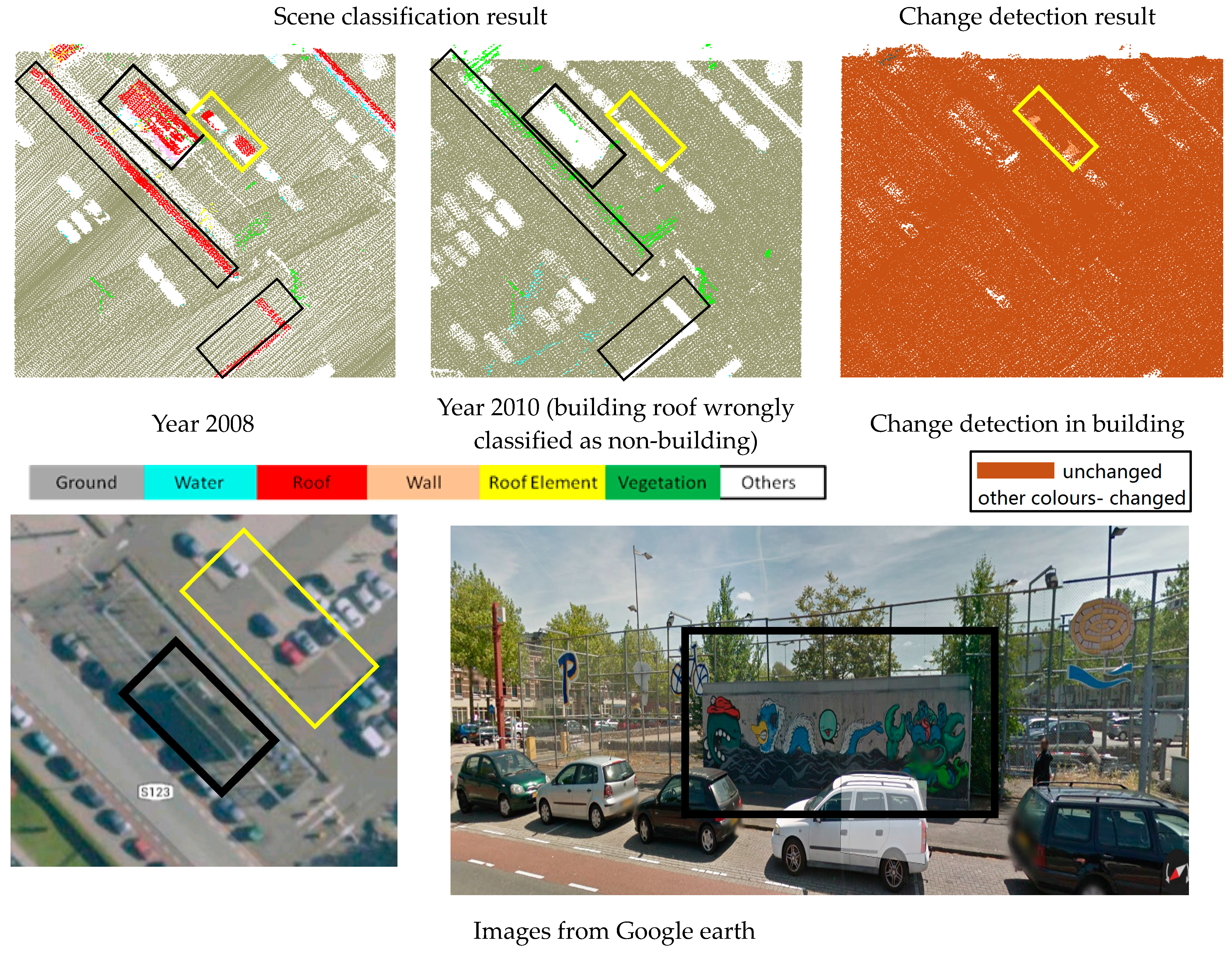
False positives occur when a change has occurred in the areas where non-building objects have been incorrectly classified as “buildings”. In the yellow rectangles shown in
Figure 14, there is an error in the scene classification of one of the epochs such that cars are incorrectly classified (in the top row) as a building roof; the water surface is also incorrectly classified as a building roof (in the bottom row). As there are changes in these areas, and one of them is incorrectly classified as part of a building, the changes are confirmed as a “change to a building”. Although these represent real changes that have occurred, they are not changes to buildings. In fact, most false positives occur with trees, when a tree is incorrectly classified as a building roof in one of the epochs.
False negatives occur when a change is confirmed but this has not been classified as being part of a building in the data sets being compared: the change will not be signalled as a “change to a building”. Some examples of false negatives resulting from scene classification errors are shown in
Figure 15. If one of the data sets is correctly classified, false negatives can be avoided.
In addition, cranes, bridges, etc., are sometimes classified as being part of a building. Nevertheless, we did not analyze changes in these objects because they did not fall within the scope of our research and we had not defined their features. Consequently, errors related to these objects have been ignored and not discussed in this paper.
5.1.4. Errors in Change Detection Due to Our Algorithm
In addition to errors propagated from scene classification results, other errors arise that are caused by limitations of the change detection algorithm used. From visual inspection, we could conclude that no changes were missed (false negatives) due to our change detection method; some unchanged walls were, however, classified as changed (false positives).
Figure 16a shows the incorrect classification of occluded walls as “changed”. We assumed that if no change to the roof of a building had occurred, the attached walls would not change either, even if they had a large difference value. Under this assumption, all wall points in the left-hand image of
Figure 16a should be labelled “unchanged”. However, there are some projections—balconies, sun shades,
etc.—on the walls that are far away from the roof, and these projections will be identified as “changed” because they have a large difference value and there was no unchanged roof found in their 2D neighborhood.
Figure 16b shows an example of what should be “unknown” points being incorrectly labelled as “unchanged”. The lack of data for the roofs in one epoch was caused by a water layer that absorbed the laser signals. In the other epoch, the point distribution is rather regular. We expected that the entire area for which data are missing would be classified as “unknown”. However, only the central part of the area was classed as “unknown” (light blue). The reason is because only the central parts of these areas in the merged data sets have a large difference value (>1.0 m radius). In other parts there are points from another epoch with a difference value less than 10 cm. Finally, these errors are not important because they did not influence the identification of the “changed” areas, they only resulted in a mix up between the designation “unchanged” and “unknown”.
Figure 14.
Scene classification errors that have no influence on the change detection results (black rectangles), and ones that have a negative influence (yellow rectangles).
Figure 14.
Scene classification errors that have no influence on the change detection results (black rectangles), and ones that have a negative influence (yellow rectangles).
Figure 15.
Examples of false negatives caused by scene classification errors. Because a building has been classified as an “undefined object” in the 2012 data set, changes to this building will not be detected (Column 3). (a) Data set 2010; (b) Data set 2012; (c) Change detection in building (merged); (d) Image from Google maps.
Figure 16.
Errors due to our change detection algorithm. Colors in this figure represent the same objects as in
Figure 15. In
Figure 16, group (1
a) shows some errors in the ellipse that are due to scene classification errors, and some in the box are due to lack of the contextual information (wall points far away from the roof). Group (1
b) shows unknown points labelled as unchanged. As seen in the classification result of Group (1b, left-hand), there is a lack of data (some holes) due to limited reflection (red) in the left-hand image of the roof, but the roof in the right-hand image is quite well covered. We expected the entire area where data is lacking to be labelled “unknown”, but in the result in (2) only the central parts of the “gaps” are “unknown” (light blue), while other parts are labelled “unchanged” (brown).
5.2. Change Classification
5.2.1. Results
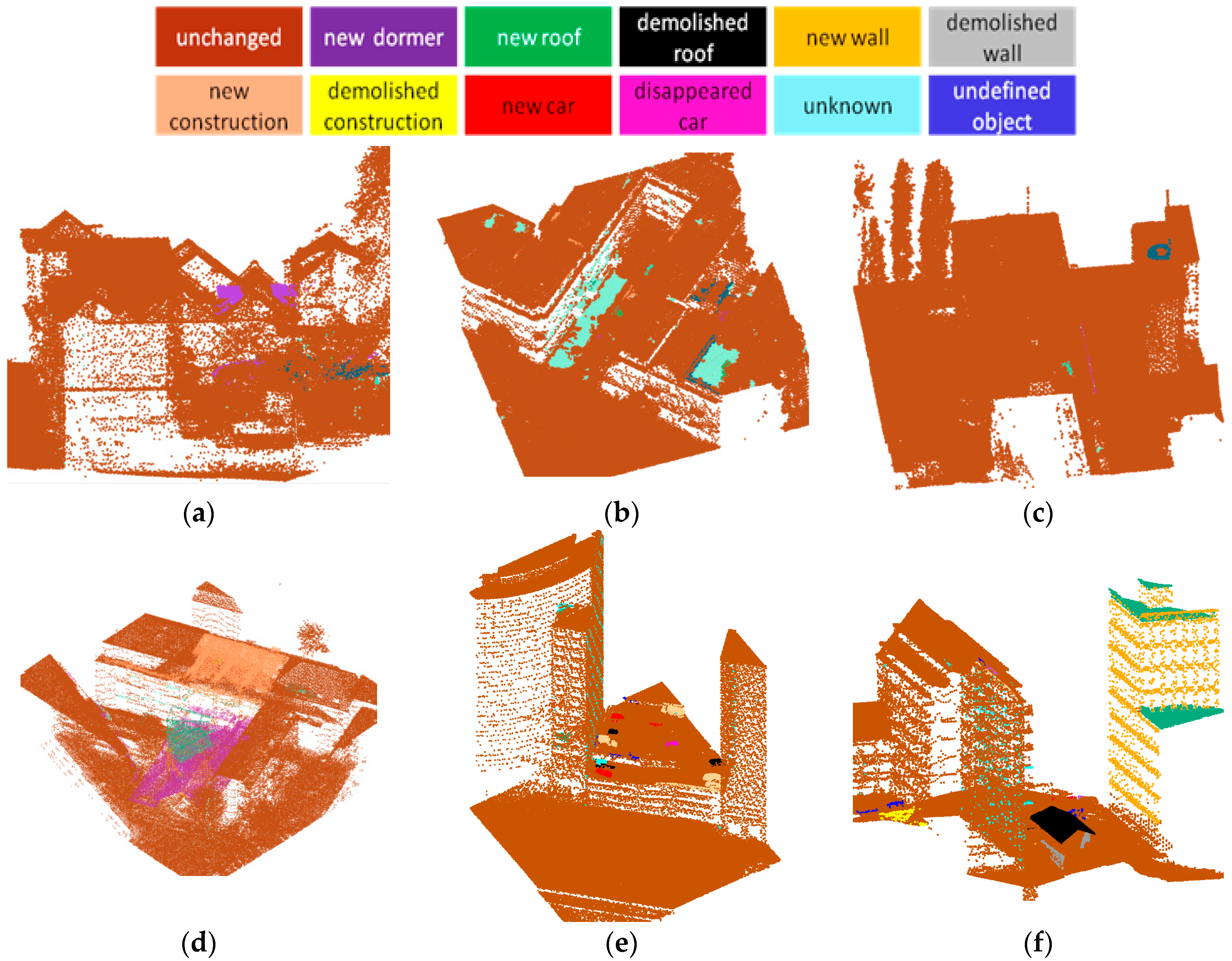
The change classification results for the two test areas are visualized in
Figure 17; for examples with a higher level of detail see
Figure 18. We chose several sites where changes were successfully detected and properly classified. These sites included examples of: (a) newly built dormers on roofs; (b) lack of data for roofs in one epoch (unknown) and lack of data for walls and ground because of occlusion; (c) undefined changes on roofs; (d) newly built constructions above roofs; (e) cars parked on top of buildings; (f) newly built and demolished buildings (two examples in one image); (g) add-on building constructions; and (h) insulation layers added to roofs.
Figure 17.
Classification of change in the test areas. (a) 2008 vs. 2010, (b) 2010 vs. 2012.
Figure 17.
Classification of change in the test areas. (a) 2008 vs. 2010, (b) 2010 vs. 2012.
Figure 18.
Successfully detected and classified examples of change. (a) newly built dormers on roofs, (b) lack of data for roofs in one epoch (unknown) and lack of data for walls and ground because of occlusion, (c) undefined changes on roofs, (d) newly built constructions above roofs, (e) cars parked on top of buildings, (f) newly built and demolished buildings (two examples in one image), (g) add-on building constructions, (h) insulation layers added to roofs. (i) new building roof under trees.
Some change detection errors are also caused by errors in scene classification—in addition to those arising from the limitations of our algorithm. These are discussed in Subsection 5.1.2. More false positives are observed, lowering the accuracy, which is analyzed in
Section 5.3.
5.2.2. Error Analysis
We randomly chose another 20 tiles with different changes from each study area to cover all types of changes on roofs. Error analysis of the change classification was done by manually assessing the correctness and completeness of changes detected (see
Table 6).
Table 6.
Completeness and correctness of the changed objects.
Table 6.
Completeness and correctness of the changed objects.
| Label | 2008 vs. 2010 | 2010 vs. 2012 |
|---|
| Correctness | Completeness | Number of Objects | Correctness | Completeness | Number of Objects |
|---|
| Undefined object | 91% | 35% | 29 | 100% | 26% | 23 |
| New dormer | 6% | 100% | 1 | 80% | 24% | 17 |
| Demolished dormer | - | - | 0 | - | - | 0 |
| New car on roof top | 33% | 11% | 9 | 50% | 7% | 14 |
| Car no longer on rooftop | 100% | 100% | 1 | - | - | 0 |
| New construction on rooftop | 13% | 25% | 8 | 42% | 56% | 9 |
| Demolished construction on rooftop | 100% | 40% | 5 | - | 0% | 2 |
| New roof | 78% | 81% | 26 | 59% | 100% | 17 |
| Demolished roof | 91% | 100% | 20 | 90% | 100% | 18 |
| New wall | 100% | 100% | 8 | 100% | 100% | 7 |
| Demolished wall | 100% | 100% | 8 | 100% | 100% | 4 |
The accuracy of change classification for roofs and walls is high compared to other objects because changes to roofs and walls occur most often in buildings undergoing entire change. In addition to that, scene classification is more reliable for larger objects: changes to buildings are generally large and can easily be correctly classified. Small changes are not so easily separated into their correct change classifications. Most constructions and undefined objects on rooftops are incorrectly classified as new or demolished dormers, especially if they are near a pitched roof. We have assumed that dormers are normally located near the pitched roof, but often roofs are in fact a combination of flat and pitched roofs, and there are as many changes on these roofs, which are not changed dormers but incorrectly classified as dormers. It is also difficult, based only on their size, to distinguish large cars on a rooftop parking lot from building constructions. As a result, some of these large cars are classified as constructions. We conclude that, even if the changes are detected correctly, in highly complex urban areas it is hard to completely and correctly classify the detected changes using geometrical and relational rules.
5.3. Object-Based Analysis
5.3.1. Results
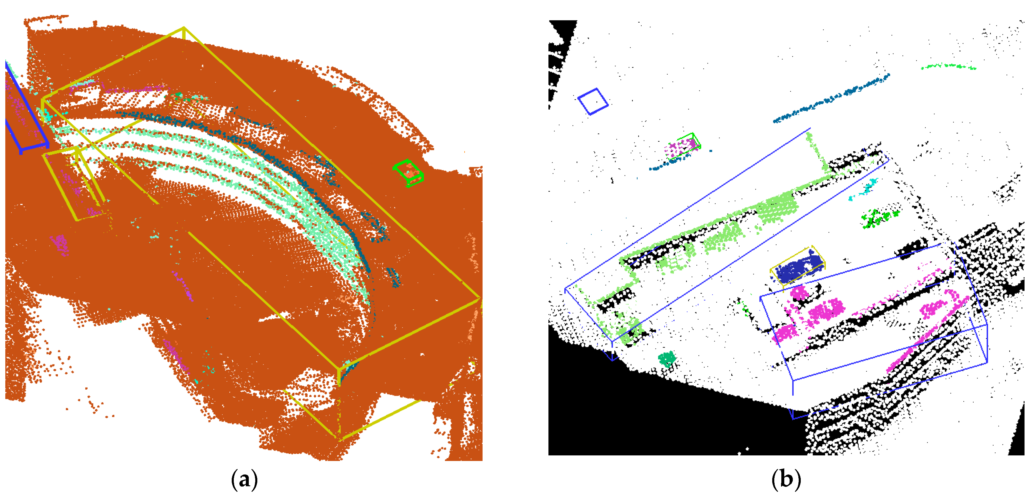
Minimum 3D bounding boxes are generated around the connected components to enable selection of relevant changes in the buildings; for some results see
Figure 19. The location of the center point, the area, and the volume of the minimum 3D bounding box are calculated. Changes are shown in
Figure 19a.
Figure 19b,c give two examples of 3D bounding boxes:
Figure 19b shows a building object that has undergone complete change; and
Figure 19c shows a changed building element (newly built dormer). The bounding box in
Figure 19c is larger than the dormer because of the influence of some outliers occurring in the same plane as the dormer.
Figure 19.
3D bounding boxes and the center points of the relevant changes, together with the calculated area and volume; the label, area and the volume are shown in the point number window. In this figure, points without bounding boxes are irrelevant changes. (a) 3D bounding boxes for the two test areas; (b) an example of 3D bounding box for an entire new building; (c) an example of 3D bounding box for newly built dormers.
5.3.2. Error Analysis
We used connected component labelling to form objects and their 3D bounding boxes to estimate their area and volumes. We found that connected component labelling failed to correctly form objects under two circumstances:
(1) False positives in buildings
Sometimes points on walls or roofs are false positives. These points may belong to an unchanged wall that has been incorrectly detected as changed (see discussion in Subsection 5.1.4), or they can be sparse points of plants on a balcony or rooftop (irrelevant changes). If such points are close together, connected component labelling will form an object that is as big as an entire wall or even a complete building; see
Figure 20a.
(2) Small objects that are too close to each other
Small objects that are too close to each other will be connected together as one object. This often occurs with cars parked on rooftops of buildings and shelters at bus stops that are very close to each other.
Figure 20b shows an example of cars parked on a rooftop. The consequence is an incorrect shape of detected change.
Figure 20.
3D bounding boxes of some wrong changes and irrelevant changes. (a) Incorrect changes in walls and irrelevant changes on roofs; (b) Cars that are close to each other and close to some fences are grouped to large objects. Yellow cubes are show objects classified as new buildings. Blue cubes are new unknown objects. Green cubes are new constructions on top of the roof.
6. Conclusions
In this paper, we present a method for detecting and classifying changes to buildings by using classified and well registered (strip difference <10 cm) laser data from several epochs. The analysis of our results leads us to draw several conclusions.
Provided distances between surfaces are greater than 10 cm and the area of change more than 4 m2, both large and small changes can be automatically detected using a surface difference map and a rule-based change detection algorithm. Areas classified as “unknown” can be correctly identified in cases of occlusions and water reflection. The surface difference map is not affected by the point density of the compared data sets. Some of the other parameters, such as the number of points indicating the approximate area and radius for the surface growing method, should be adjusted with varying point densities.
Larger changes can be correctly assessed as belonging to a building provided that building has been correctly classified as such in the scene classification step for one of the data sets being compared. The accuracy of object recognition was evaluated by overlaying the 3D bounding boxes of the buildings for which change was detected on manually generated reference data. Our method detected 91% of actual changes in Test area 1 and 83% in Test area 2. Nearly half of the changes detected in objects were irrelevant changes.
About half of the false positives that occurred were caused by scene classification errors. The other false positives can be mostly attributed to our change detection algorithm. Mostly they are spurious changes in a wall that is at a larger distance to a roof, plants growing in a rooftop garden, containers, isolation layers, cleaning machines on the top of buildings, etc. Regarding classifying changes, we conclude that ,even if changes are identified correctly, in highly complex urban areas it is difficult to completely and accurately classify the smaller detected changes using geometrical and relational rules.
The classification result for the changed object shows that large changes affecting an entire building, for example its roof or a main wall, can be detected with a higher degree of accuracy than changes made to a building element, such as dormers or construction on top of the building.
Overall, our method detected 80-90% of changes to buildings. It is the first time that we tried to detect high-level detail changes in buildings using raw lidar data, so we did not compare our accuracy to other methods. Our method is, however, not yet capable of distinguishing small irrelevant changes to objects from relevant ones. A more accurate definition of a “changed building object” and its characteristics are required in order to better interpret differences between two data sets.


