Quality Assessment of Roof Planes Extracted from Height Data for Solar Energy Systems by the EAGLE Platform

Abstract

Due to the increasing scarcity of fossil fuels and the upwards trend in energy costs over time, many countries—especially in Europe—have begun to modify their energy policies aiming to increase that percentage obtained from renewable energies. The EAGLE (FP7 program, European Commission) has developed a web-based platform to promote renewable energy systems (RES) in the public and private sectors, and to deliver a comprehensive information source for all interested users. In this paper, a comprehensive quality assessment of extracted roof planes suitable for solar energy installations (photovoltaic, solar thermal) from height data derived automatically from both LiDAR (Light Detection and Ranging) and aerial images will be presented. A shadow analysis is performed regarding the daily path of the sun including the shading effects of nearby objects (chimneys, dormers, vegetation, buildings, topography, etc.). A quality assessment was carried out for both LiDAR and aerial images of the same test sites in UK and Germany concerning building outline accuracy, extraction rate of roof planes and the accuracy of their geometric parameters (inclination and aspect angle, size). The benefit is an optimized system to extract roof planes for RES with a high level of detail, accuracy and flexibility (concerning different commonly available data sources) including an estimation of quality of the results which is important for individual house owners as well as for regional applications by governments or solar energy companies to judge their usefulness.

1. Introduction

1.1. Background

The 21st century has so far been characterized by an increasing scarcity of fossil fuels and an associated significant increase in energy costs. Coupled with concerns to do with nuclear energy, many countries—especially in Europe—have begun to explore the potential of renewable energies, and to modify energy policy accordingly. The European Commission (EC) supported the EAGLE project “Development and demonstration of a dynamic, web-based, renewable energy rating platform” (No. 286161) as part of the FP7 program [1]. The aim of this is the acceleration of market penetration of Renewable Energy Systems (RES) in both industrial and domestic sectors. RES can make use of existing built-up areas, e.g., utilizing building roofs for photovoltaic or solar thermal energy harvesting. However, one of the main obstacles may be the uncertainty over returns on investment. Therefore, the objective of the research presented here was to provide accurate and objective information about the suitability of roof areas for RES in an automatic manner. Two target groups have been defined: at one scale regional and national government institutions and solar energy companies for regional applications, at another finer scale individuals like RES suppliers and installers as well as house owners who need suitability information about a locality with a higher level of detail (e.g., regarding chimneys, dormers etc.).

In this paper, the main focus is a comprehensive quality assessment of roof planes extracted from both LiDAR and aerial imagery. In the literature, suitable evaluation systems have been developed for this purpose concerning different aspects like detection rates and geometric accuracy. Research on data availability in Europe has shown that a nationwide coverage of LiDAR data is only realized by a few countries and the update cycles are (mostly) irregular with long time intervals. Therefore, the system must be able to alternatively derive height data automatically from aerial images which are acquired more regularly with higher coverages (approaching 100%) over relatively short time intervals (three to five years) by almost all European countries. Additionally, building outlines (e.g., from cadastral data or other databases) are used to restrict the processing to built-up areas and to accelerate the extraction of large areas (e.g., 100 km² or more). These data are available in all European countries and regularly updated.

1.2. Related Work

One of the main components of all systems based on remote sensing for the detection and modelling of buildings is the extraction of roof structures. Our focus here is on the development of such a system for the extraction of roof areas for solar energy installations, where relatively few publications can be found. In addition, we also describe some existing approaches for quality assessment appropriate to the context of this paper.

1.2.1. Roof Plane Extraction

Almost all approaches for roof reconstruction are based on the assumption that roof structures can be approximated by planar faces (e.g., Dorninger and Pfeifer [2]). On the one hand, they can be distinguished by the input data the algorithms are adapted for, on the other hand, by the underlying methodology. In respect to input data, only a few approaches use multiple aerial images to extract roof planes, e.g., Noronha and Nevatia [3]. The vast majority make use of airborne LiDAR (Light Detection and Ranging) data for this purpose due to significantly fewer problems (e.g., Oude Elberink [4]). For the approaches based on LiDAR data, a comprehensive overview is given in Vosselman and Maas [5]. In most cases, a pre-processing is carried out to separate ground points from above-ground points. In general, we can distinguish between model-driven and data-driven approaches (e.g., Tarsha-Kurdi et al. [6,7]).

Model-Driven Approaches

Model-driven methods make use of pre-defined parameterized prototypes of building models from a library, and perform a best-fit of every stored model to the point cloud to determine the values of the building parameters (length, width, height, roof slope etc.). The model with the smallest residuals is chosen. Although closed and topologically consistent 3D models are obtained, this is at the expense of flexibility concerning non-standard building shapes. One of the first approaches developed was such a model-driven procedure proposed by Weidner and Foerstner [8], restricted to buildings with flat and gable roofs. Other approaches use invariant moments to obtain a closed solution (Maas and Vosselman [9]). Further examples of model-driven algorithms can be found in Tarsha-Kurdi et al. [7]. These approaches are preferable for low point densities (e.g., Jochem et al. [10]).

Data-Driven Approaches

Data-driven methods extract object primitives (e.g., walls, roof planes etc.) and combine them to produce a final 3D model, however this may be inaccurate due to missing or erroneous building parts. These methods are more suitable for dense point clouds (e.g., >15 pts./m²) as these can resolve details of roof structures (e.g., chimneys, dormers etc.). This may explain why the various types of data-driven methods have been increasingly adopted. They can be distinguished by their methodological strategies. For instance, Schwalbe et al. [11] created an interesting approach based on orthogonal projections of the point cloud regarding the main orientation of the building and the extraction of straight lines representing roof planes in 2D, while Tarsha-Kurdi et al. [12] extract roof planes by applying the RANSAC (Random Sample Consensus) algorithm. However, numerous researchers have used region growing algorithms for roof plane extraction, differentiated by the kind of seed point definition and homogeneity criteria employed. The similarity of normal vectors representing the local homogeneity of the surface is exemplified by Rottensteiner et al. [13], Dorninger and Pfeifer [2], Jochem et al. [14]. Oude Elberink and Vosselman [15], and Xiong et al. [16] use the 3D Hough space to detect seed points and topology graphs to model the relationships among the extracted roof planes, which can also handle incomplete data due to missing LiDAR points. A similar approach is introduced by Perera et al. [17]. Straight ridge lines and step edges are extracted to create a so-called roof topology graph for the reconstruction of roof structures. Awrangjeb et al. [18] perform an eigenvalue analysis for the extraction of coplanar points to find seed points of a subsequent region growing process. For this task, in most cases, the distance between a LiDAR point and the hitherto extracted plane is taken as the homogeneity criterion.

Approaches Using Additional Information

Several researchers have combined LiDAR and aerial image data due to additional information such as spectral reflectance and texture features to stabilize the reconstruction process (e.g., Rottensteiner and Brise [19]; Rottensteiner et al. [20]; Brenner [21]; Novacheva [22]; Awrangjeb et al. [18]). Others additionally use building outlines (e.g., from cadastral data) to support the subsequent extraction of roof planes (e.g., Brenner and Haala [23]; Vosselman and Dijkman [24]; Schwalbe et al. [11]).

Even if there are some significant problems of reconstructing buildings and roof structures, as discussed in Oude Elberink [4], the capability and efficiency of modern approaches could be demonstrated by the EuroSDR comparison (Kaartinen et al. [25]) and the ISPRS benchmark tests [26].

1.2.2. Suitability of Roof Planes for RES

Compared to the considerable number of methods for 3D building and roof reconstruction, only relatively few approaches can be found related to the specific challenge of determining the suitability and potential of roof planes for renewable energy systems (RES), specifically photovoltaic and solar thermal energy. Here, the main factors which have to be represented are: (i) the path of the sun; (ii) inclination and aspect of solar radiation on the roof plane; (iii) global radiation and (iv) the resulting shadowing effects of topography and nearby objects (Šúri and Hofierka [27]). Wittmann et al. [28] were one of the first researchers to use aerial images for the identification of roof areas suitable for installation of RES, although they applied manual photogrammetric measurements to derive the necessary roof plane parameters. The first automatic approach based on LiDAR data and building outlines was presented by Voegtle et al. [29] (cf. Section 2.1.2). Kassner et al. [30] exclusively made use of publicly available LiDAR data and building outlines for masking LiDAR points on the roofs. Therefore, only a limited point density of ≤1 pt./m² was achieved. This pixel-based approach made use of GIS to determine the roof plane parameters, which were then included in a quality assessment, reporting the percentage of correctly and falsely identified roof areas. As a reference, CAD models of 13 buildings were measured by classical stereo photogrammetry (Analytical Plotter) to obtain the real shape without generalisation (in contrast to cadastral data). Jochem et al. [10,14] have developed an approach based on high density (17 pts./m²) LiDAR point clouds and the plane extraction method mentioned in Section 1.2.1. Here, the size of the individual roof facets is derived from contour lines generated by means of so-called alpha shapes [31]. A refinement of shadow analysis is carried out by including transparency values for nearby vegetation objects based on penetration rates derived from the LiDAR returns. A sophisticated determination of energy yield is described in detail. In context of the project SUN AREA, Ludwig et al. [32] created a method for estimation of the solar potential of individual buildings as well as for large regions (>100 km²). Using LiDAR data (4 pts./m²) as input and cadastral building outlines, a raster-based selection of homogeneous areas is performed by applying multiple thresholding which leads to a segmentation of areas with uniform inclination and aspect angles. Deviations from the optimal values (inclination: 37°, aspect: south) are obtained by reduction factors derived from meteorological investigations. This relatively simple approach can be applied to large regional areas, e.g., the city of Osnabrueck (Germany) covering approx. 120 km². In Agugiaro et al. [33,34], aerial images are also used in addition to LiDAR data to derive digital surface models (DSM) of different resolutions (1.0 m, 0.25 m). The raster-based analysis of inclination, aspect, size and shadowing effects of mountainous topography and nearby buildings is based on a common GIS (GRASS) and its functions (e.g., “r.sun”). For quality assessment, 30 reference roofs are measured manually. The results of usable solar radiation obtained from different input raster data mentioned above are then compared. Gooding et al. [35] have created a model-driven approach especially for low point densities by grouping similar buildings together to increase the number of points on the roof structures. The quality evaluation delivers an identification rate of 87% and a mean absolute error of 3.76° for roof slopes.

1.2.3. Quality Evaluation

There are various approaches to image-based quality evaluation. These can be distinguished by the number and types of different quality parameters used: a good survey is provided by Foody [36] in the general context of land cover classification. In the specific context of this paper, a very good overview of existing quality evaluation methods is given by Zeng et al. [37] who observe that a common approach that they describe as matched rates employs parameters originally derived from image classification (Foody [36]), i.e., completeness, correctness and quality. These are determined based on reference models (e.g., Rutzinger et al. [38]; Truon-Hong and Laefer [39]). These parameters can also be applied to extracted roof planes. The second approach considered by Zeng et al. [37] is shape similarity which describes a more complicated category of metrics which may be subjective and poorly defined especially for complex shapes. For this, metrics like area and perimeter difference (Song and Haithcoat [40]), tangent function or moment-derived parameters can be used. Other researchers have compared each segment of a contour line by checking if it lies inside a buffer zone around the corresponding segment of the reference model (Truong-Hong and Laefer [39]). The last approach identified by Zeng et al. [37] is positional accuracy which is often determined by the root mean square error (RMSE) for comparing any extracted information and a higher accuracy reference, frequently employed in other areas of geospatial processing such as DEM quality assessment (e.g., Fisher and Tate [41]). It is clear from the literature that many different parameters have to be used, however, these may be strongly correlated and it is difficult to use many of these simultaneously. One response exemplified by Zeng et al. [37] is to develop a multi-criteria evaluation method due to ambiguities and errors when using simple metrics. This sophisticated evaluation system incorporates different quality measures like geometric elements (shape, displacement) in addition to the more common detection rates in a hierarchical structure.

The remainder of this paper is structured in the following way: in Section 2, we present the methodology of extracting roof planes suitable for solar energy installations and the measures of quality assessment. In Section 3, the results of a comprehensive quality assessment are described, whilst in Section 4, these results are discussed. In Section 5, we present some conclusions and an outlook to future developments.

2. Methods

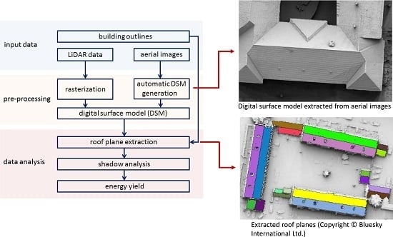
2.1. Extraction Approach

The extraction approach of EAGLE was designed to use both LiDAR data as well as height data derived automatically from aerial images as an alternative data source (Figure 1). Therefore, the system has two different pre-processing paths until height data in a suitable format (DSM) are generated. From this point, all subsequent processing steps are identical. The first step in the data analysis is the extraction of planar roof areas and their geometric parameters (slope, aspect, size). To accelerate roof plane extraction, building outlines are used as complementary input data. The final two steps comprise a shadow analysis to estimate the reduction of solar radiation on each roof plane (e.g., by nearby objects, surrounding buildings etc.; Schuffert [42]) and the calculation of energy yield.

Figure 1. Principle workflow of the system for extraction of suitable roof planes for solar energy installations. LiDAR or aerial image data can be used. Building outlines are introduced to mask out prospective roof areas.

Figure 1. Principle workflow of the system for extraction of suitable roof planes for solar energy installations. LiDAR or aerial image data can be used. Building outlines are introduced to mask out prospective roof areas.

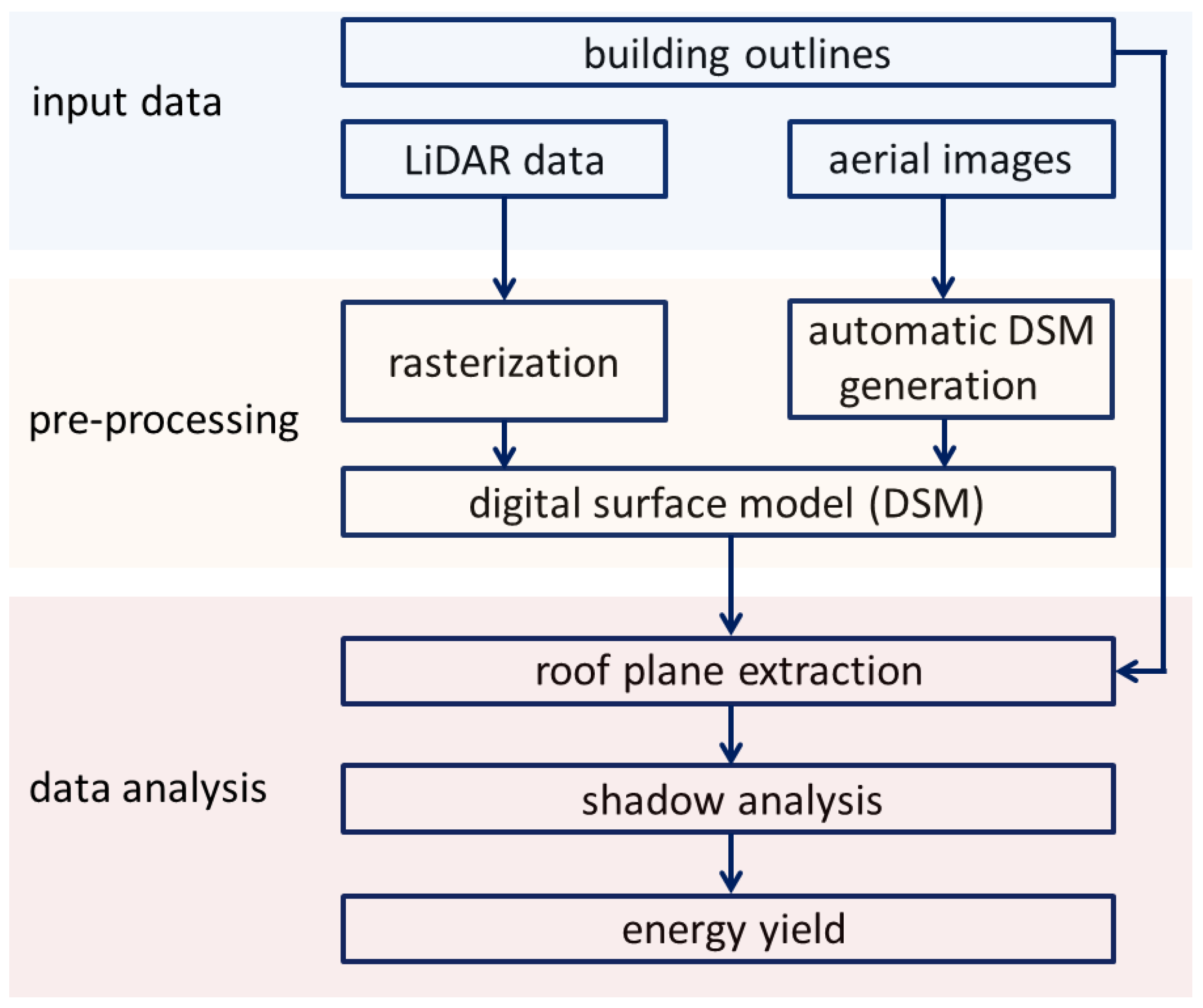
2.1.1. Data Pre-Processing

If LiDAR data are available—preferably with a point density of >2 pts./m²—pre-processing is limited to a rasterization of the LiDAR point cloud. This decreases noise and is computationally more efficient, albeit with a trade-off in an associated reduction in quality through generalization or loss of some small object details in the rasterization process. In the cases where aerial images are taken as input data, more extensive pre-processing has to be carried out. The exterior orientation of the images as well as the interior orientation of the camera must be known or determined by a bundle adjustment. Country-specific interfaces have been created in EAGLE for the different input formats.

2.1.2. Roof Plane Extraction

For the extraction of planar surfaces numerous approaches can be found in the literature (cf. Section 1.2.1). In the EAGLE system, a method based on a region growing approach is implemented from work presented in Voegtle et al. [29]. For detection of a seed pixel, the heights of its local surrounding pixels (e.g., N8 neighborhood) must fulfill the equation of a plane (Equation (1)):

$$z \left(x,y\right)= a_0+a_{1}x+a_{2}y$$

(1)

where z (x,y)—height at position (x,y); a_i—plane parameters with only small acceptable differences:

$$d_{P_i}= \widehat{z} \left(x,y\right)- z_i\left(x,y\right)$$

(2)

where $\widehat{z}$—height value of the plane; z_i—height of LiDAR point i.

If Σ d_Pi < t (e.g., t = n·σ; n—number of surrounding pixels, σ—noise level of input data) of the local neighbourhood is fulfilled, this point will be accepted as a seed point. After a seed point is found, all adjacent pixels are statistically tested to determine whether the height values z_i fit to the previous plane, i.e., their height difference d_Pi with respect to the points of the current plane. This test value t is defined as:

$$t=\left|\overline{d}-d_{Pi}\right|\sqrt{\frac{n}{\left(n+1\right)s^2}}<t_{1-\frac{a}{2},f}$$

(3)

$\begin{array}{cccc}\text{where}\hfill & \hfill \overline{d}\hfill & \hfill -\hfill & \text{mean distance of the current plane points to the plane}\hfill \\ \hfill & \hfill n\hfill & \hfill -\hfill & \text{number of current plane points}\hfill \\ \hfill & \hfill s^2\hfill & \hfill -\hfill & \text{variance of current plane points}\hfill \\ \hfill & \hfill t_{1-\frac{a}{2},f}\hfill & \hfill -\hfill & \text{quantile of Student’s }t\text{ distribution of level of significance α and degree of freedom }f\hfill \end{array}$

The main advantage of this test (Student t test)—compared to a fixed pre-defined threshold—is an automatic adaption of the acceptable point distance to the current plane. At the beginning of the region growing process, when only a few points had been found, larger point distances to the plane are accepted automatically, whereas at a later stage, when a large number of points belong to the plane and its spatial position and orientation has been stabilized, a new point might have only a small distance to get accepted. If no new points can be found which fulfill the defined condition, the process stops, the area found is marked and a new seed point will be detected. To accelerate this process and to exclude other objects like trees, the seed points are located inside the building outlines (e.g., obtained from cadastral data). Due to the remaining inaccuracies of the input data and roof overhangs (eaves), certain displacements may occur between the building outlines and LiDAR or aerial image data (cf. Section 2.2). Therefore, a buffer of sufficient size is created around the outlines to enable the region growing to cover the entire roof area.

2.1.3. Geometric Roof Plane Parameters

To determine the suitability of roof planes for solar energy installations, three geometric parameters are essential: slope angle α and aspect angle γ as well as size. The first two parameters can be easily determined by the coefficients a₁ and a₂ of the mathematical description of an extracted plane j (cf. Equation (1)):

$$slope {\alpha }_j= \sqrt{a_1^2+ a_2^2} aspect {\gamma }_j= \frac{a_1}{a_2}$$

(4)

The size can be derived by the number of pixels or alternatively, by a boundary polygon of a roof area, e.g., generalised by the well-known Douglas-Peucker algorithm (Douglas and Peucker [43]) or other suitable methods (e.g., alpha shapes, Jochem et al. [14]). In each case, the real area A_j of an oblique plane j has to be calculated from this planimetric area A_pj by means of the inclination angle α_j (Equation (4)).

$$A_j=\frac{A_{p_j}}{cos \left({\alpha }_j\right)}$$

(5)

2.1.4. Further Processing

Although not within the immediate scope of this paper, we mention in passing the additional processing steps to contextualise our work as part of the EAGLE system. Shadowing is one of the most important influences restricting the economical use of solar energy installations. Therefore, a comprehensive and detailed shadow analysis related to each individual roof plane is essential. For this, it is necessary to include the DSM data beyond local objects like dormers and chimneys, such as adjacent buildings as well as the underlying topography. The shadow analysis implemented in the EAGLE system determines in a first step a series of date- and location-dependent incidence angles of the sun during a day in short time intervals, e.g., 15 min according to the smooth path of the sun (e.g., Meeus [44]). By the intersection of these incidence angles with the DSM, shadowing effects and their duration can be determined for each pixel of a roof plane. Shadow analyses are computationally extremely time-consuming (e.g., Agugiaro et al. [33]). Due to the smooth change of the sun paths during a month, the shadowing effects do not need to be calculated for each single day but only for appropriate time intervals, e.g., five days or 10 days: the effects on days in between can be interpolated. This approach leads to significant efficiencies. The resulting shadowing effects are regarded as a reduction factor which is determined by the ratio of the time without shading and the maximum time of sun radiation during a given interval, e.g., one month. Due to the local impact of disturbing objects like chimneys or dormers on their direct neighbourhood, the determination of shadowing effects is carried out for each pixel of the roof area. In Figure 2, an example of such a shadow analysis is presented for two different seasons (June, December) where significant differences are recognizable.

Figure 2. Color-coded shadowing effects on the roof areas of the Karlsruhe (GER) test site (subset) for different months (green = no effects, red = strong effects). (a) DSM; (b) June; (c) December. Copyright: Grundlage: Auszug aus dem Digitalen Oberflächenmodell—© Landesamt für Geoinformation und Landentwicklung Baden-Wuerttemberg (www.lgl-bw.de), 04.12.2014, Az.: 2851.3-A/854.

Figure 2. Color-coded shadowing effects on the roof areas of the Karlsruhe (GER) test site (subset) for different months (green = no effects, red = strong effects). (a) DSM; (b) June; (c) December. Copyright: Grundlage: Auszug aus dem Digitalen Oberflächenmodell—© Landesamt für Geoinformation und Landentwicklung Baden-Wuerttemberg (www.lgl-bw.de), 04.12.2014, Az.: 2851.3-A/854.

For the next processing step—the estimation of energy yield for each roof plane—several alternatives can be applied. One solution is the use of a matrix of reduction factors according to the deviation of a roof plane from the optimal spatial orientation (aspect: south, slope: 38°), e.g., in steps of 2°. Values between these nodes will be interpolated. The reduction values are determined by long-term research of solar panel experts. Other researchers have developed specific formulae where besides the geometric parameters, also the statistical meteorological data of the given location are input to estimate the expected energy yield.

2.2. Evaluation Strategy

A comprehensive quality evaluation has to incorporate a variety of different measures (e.g., Zeng et al. [37], Truong-Hong and Laefer [39]). For this application of solar energy installations on rooftops, several commonly used measures are used: the geometric coincidence of building outlines (e.g., cadastral data) and height data (DSM), extraction rates of roof planes (completeness, correctness, quality) and the accuracy of the geometric plane parameters (slope, aspect, size). In addition to these, we include the influence of data resolution and compression rate on the extraction results.

Cadastral building outlines are used in this approach as complementary input data. Hence, the geometric coincidence of building outlines and their borders in height data (LiDAR DSM or automatically extracted DSM from aerial images) is an important issue in quality assessment. Certain discrepancies may occur caused by errors in the geo-referencing of the LiDAR data, or in the exterior orientation of the aerial images. Dependent on the data source, building outlines may also contain positioning errors and generalization effects. Additionally, roof overhangs have to be taken into account, which are normally not incorporated into building outlines from cadastral data. For an automated determination of these differences, maximum gradients along building edges are extracted from the height data (DSM) in the first step (e.g., by the well-known Laplace/Laplace of Gaussian (LoG) operator). In the second step, the shortest (orthogonal) distances of the position of the maximum gradient to the related polygon line of the building contour are calculated. These distances can be used to determine the mean and the maximum value.

The quality of roof plane detection can be described by the common parameters completeness (compl), correctness (corr) and quality (qual), e.g., Zeng et al. [37], Truong-Hong and Laefer [39]. If the pixels of an extracted roof plane cover the corresponding reference area by more than 20% (to exclude artefacts), the center of gravity is determined and this plane is counted as T_p. If no center of gravity can be found inside a reference plane, this is counted as F_n according to e.g., Jochem et al. [14] and Rutzinger et al. [38]. F_p is derived from the number of extracted planes not (entirely) usable for solar energy installations. These correspond either to extracted planes inside the building contour line whose center of gravity lies in none of the reference areas (e.g., yard area, atrium etc.), or extracted planes containing undetected disturbing objects (dormers, chimneys).

$$compl= \frac{{{\displaystyle \sum }}^{\text{}}{T}_p}{{{\displaystyle \sum }}^{\text{}}{T}_p+ {{\displaystyle \sum }}^{\text{}}{F}_n} corr= \frac{{{\displaystyle \sum }}^{\text{}}{T}_p}{{{\displaystyle \sum }}^{\text{}}{T}_p+{{\displaystyle \sum }}^{\text{}}{F}_p} qual= \frac{{{\displaystyle \sum }}^{\text{}}{T}_p}{{{\displaystyle \sum }}^{\text{}}{T}_p+{{\displaystyle \sum }}^{\text{}}{F}_n+{{\displaystyle \sum }}^{\text{}}{F}_p}$$

(6)

where: T_p—True positives (correctly detected roof planes); F_n—False negatives (undetected roof planes); F_p—False positives (planes outside reference areas and planes with undetected; disturbing objects).

As described in Section 2.1.3, the inclination and aspect angle as well as the size can be determined for each extracted roof plane. For a quality assessment of these geometric parameters, reference roof planes have been obtained, by manual measurement of the aerial images in a photogrammetric workstation. A quality check based on two buildings acquired by a tachymeter has confirmed an expected point accuracy of the planes of ±0.07 m. To obtain consistent results, these reference planes have been verified independently by a second operator based on visual inspection. The deviations between reference planes (of significantly higher accuracy) and extracted planes will be used as a quality measure. To obtain the effective usable areas for solar energy installations and to guarantee a correct comparison of the related size, disturbing objects (chimneys, dormers etc.) have to be excluded in these reference data (Figure 3). Different building types and complexity levels of roof structures have been selected for this purpose.

The quality of the results of automatic image matching algorithms is highly sensitive to the degree of image texture, and therefore to the image resolution. Homogenous parts of an image may produce unreliable results or possibly gross errors. Roof areas are frequently built of one single material (e.g., identical red roof tiles) which leads to such homogenous image areas, particularly if the image spatial resolution is insufficient to capture this spatial structure. Due to the availability of two aerial image datasets with different resolutions (pixel size 0.06 m and 0.20 m) of the same test site in Karlsruhe, a comparison of the automatically derived DSMs can be done. However, because only one test site was able to be captured with different resolutions, a qualitative evaluation only was carried out at this stage.

Figure 3. Reference roof planes of the Leicester test site created by manual measurement of aerial images. (a) Aerial image; (b) Reference planes. Disturbing objects have been excluded. Copyright © Bluesky International Ltd. (Leicestershire, UK).

Figure 3. Reference roof planes of the Leicester test site created by manual measurement of aerial images. (a) Aerial image; (b) Reference planes. Disturbing objects have been excluded. Copyright © Bluesky International Ltd. (Leicestershire, UK).

In one case of our extensive data acquisition over Europe, the aerial images had been delivered firstly in a compressed status (jpeg format). After a request for an uncompressed dataset, we received the data in the original (uncompressed) format (tiff). Therefore, we were able to contrast the results of processing both the compressed und uncompressed datasets.

Lastly, since we had access to both data types (LiDAR, aerial images) for the same two test sites, extracted on the base of the same building contours, the same reference data and the same algorithm, we were able to do a qualitative comparison of each data type, commenting on the differences, advantages and disadvantages.

2.3. Data Sources and Software Environment

In context of the EAGLE project an extensive database—13 different datasets from five European countries (six LiDAR, seven aerial image data)—was sampled and processed. It can be seen that for Leicester (UK) and Karlsruhe (GER) test sites, both LiDAR and aerial image data are available. To enable a better comparison and a comprehensive evaluation of the extraction results of both data types for the same test area, the quality assessment was carried out only with these two test sites (red boxes in Table 1). The sensor types for these LiDAR datasets were an Optech ALTM Gemini (Karlsruhe, Germany) and an Optech M300 (Leicester, UK), for the aerial images an UltraCAM X (Karlsruhe, Germany and Leicester, UK).

For software development Python, Bash, GDAL and Numpy libraries were used. The automatic determination of height data (DSM) from aerial images was based on an adapted version of the MicMac algorithm (IGN, France [45]).

Table 1. Datasets processed by the EAGLE system. For the Karlsruhe test site, two different resolutions were available for classical aerial imagery as well as for unmanned aerial vehicles (UAV); datasets marked in red were used for quality evaluation.

Country	Location	Data Type	Resolution
United Kingdom	Leicester		0.25 m 0.14 m
	Bristol	LiDAR	0.50 m
	The Village	Aerial Images	0.12 m
	Slough (London)	LiDAR	0.50 m
Germany	Karlsruhe		0.50 m 0.06 m/0.20 m
		UAV Images	0.02 m/0.04 m
Sweden	Stockholm	LiDAR	0.50 m
The Netherlands	The Hague	Aerial Images	0.04 m
Spain	Madrid	LiDAR	1.00 m

Table 1. Datasets processed by the EAGLE system. For the Karlsruhe test site, two different resolutions were available for classical aerial imagery as well as for unmanned aerial vehicles (UAV); datasets marked in red were used for quality evaluation.

Country	Location	Data Type	Resolution
United Kingdom	Leicester		0.25 m 0.14 m
	Bristol	LiDAR	0.50 m
	The Village	Aerial Images	0.12 m
	Slough (London)	LiDAR	0.50 m
Germany	Karlsruhe		0.50 m 0.06 m/0.20 m
		UAV Images	0.02 m/0.04 m
Sweden	Stockholm	LiDAR	0.50 m
The Netherlands	The Hague	Aerial Images	0.04 m
Spain	Madrid	LiDAR	1.00 m

3. Results

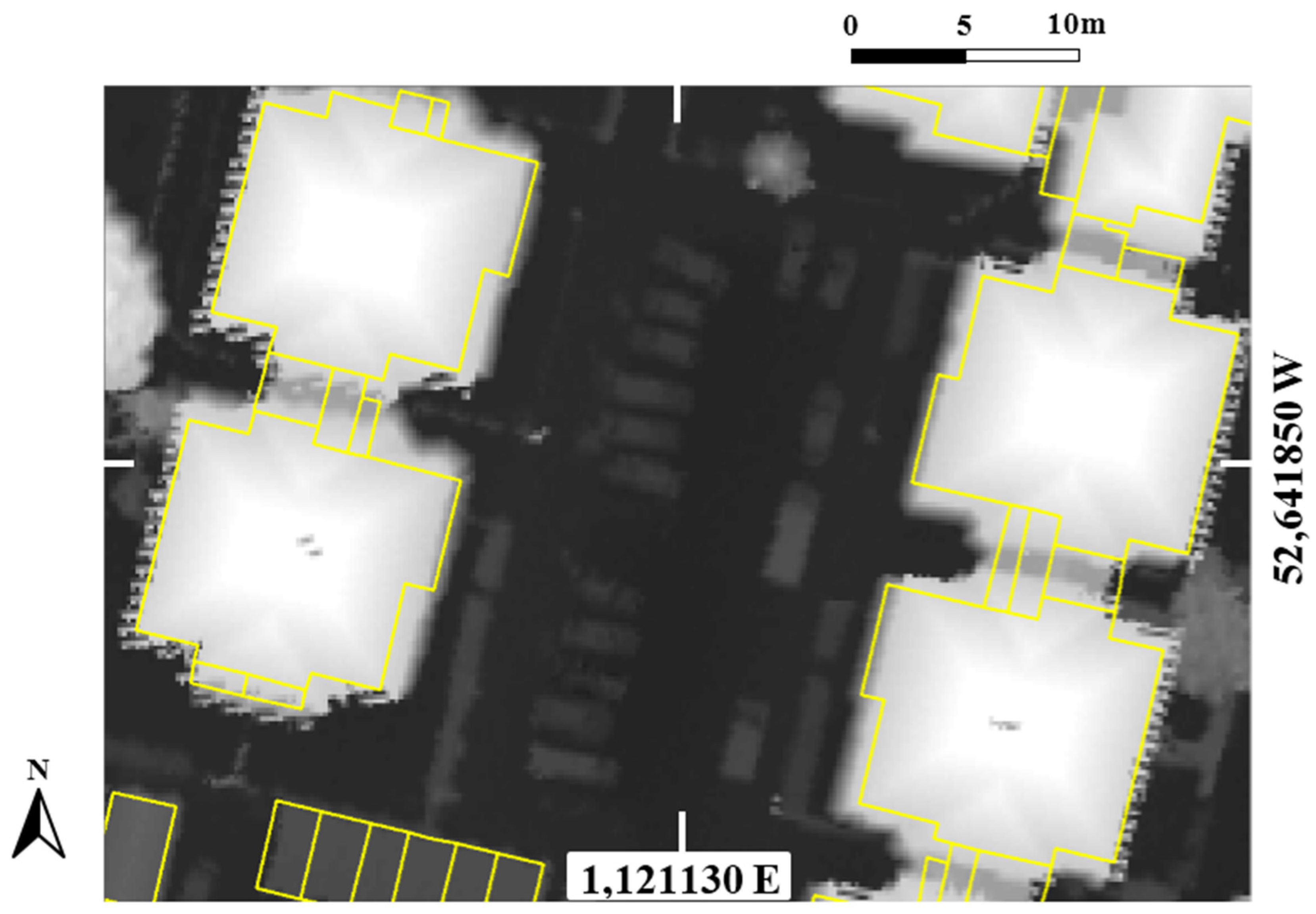
3.1. Geometric Coincidence of Building Outlines and Building Borders in Height Data (DSM)

For the evaluation of the geometric coincidence, a random sample of 30 test buildings in each test site—containing approx. 200–400 gradients per residential building, and more than 1000 gradients for larger industrial buildings—were used. The results are shown in Table 2. Several manual measurements randomly distributed at different buildings to verify these values have confirmed the results of Table 2.

Table 2. Mean distance, maximum and minimum distance and standard deviation between building outlines and their borders in the height data (DSM) for the Leicester and Karlsruhe test sites.

Test Site	Mean Distance	Max. Distance	Min. Distance	Std. Dev.
Leicester (UK)	0.92 m	1.91 m	0.06 m	0.40 m
Karlsruhe (GER)	0.73 m	1.57 m	0.03 m	0.37 m

Table 2. Mean distance, maximum and minimum distance and standard deviation between building outlines and their borders in the height data (DSM) for the Leicester and Karlsruhe test sites.

Test Site	Mean Distance	Max. Distance	Min. Distance	Std. Dev.
Leicester (UK)	0.92 m	1.91 m	0.06 m	0.40 m
Karlsruhe (GER)	0.73 m	1.57 m	0.03 m	0.37 m

For a better visualisation of these results, an overlay of the cadastral building outlines and the LiDAR data (DSM) is shown in Figure 4.

Figure 4. Overlay of cadastral building outlines and height data (raster DSM derived from LiDAR data), Leicester test site (cf. Table 1). Building outlines: © Crown copyright and database right 2012 Ordnance Survey licence number 100042840, LiDAR data: Copyright © Bluesky International Ltd. (Leicestershire, UK).

Figure 4. Overlay of cadastral building outlines and height data (raster DSM derived from LiDAR data), Leicester test site (cf. Table 1). Building outlines: © Crown copyright and database right 2012 Ordnance Survey licence number 100042840, LiDAR data: Copyright © Bluesky International Ltd. (Leicestershire, UK).

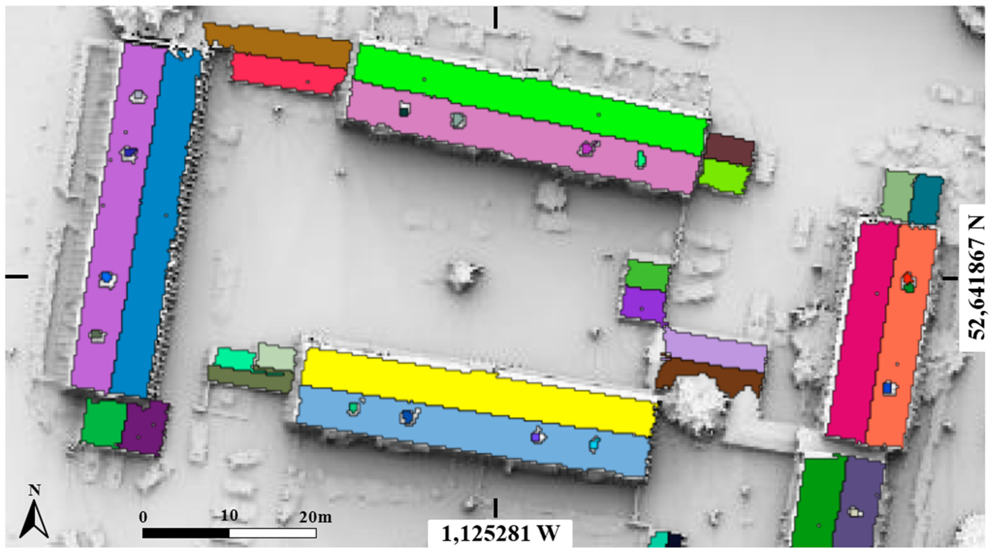
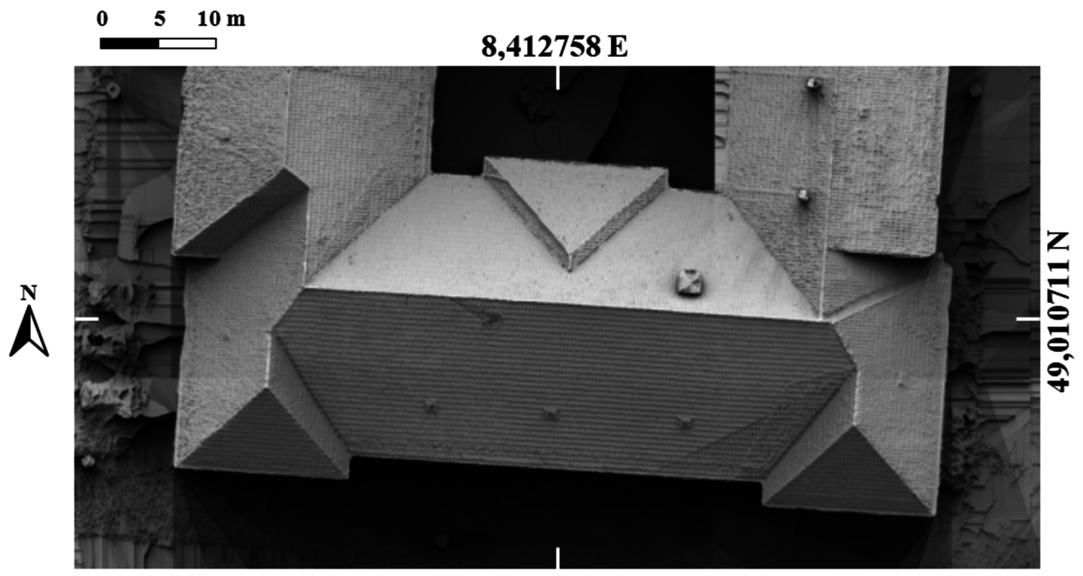
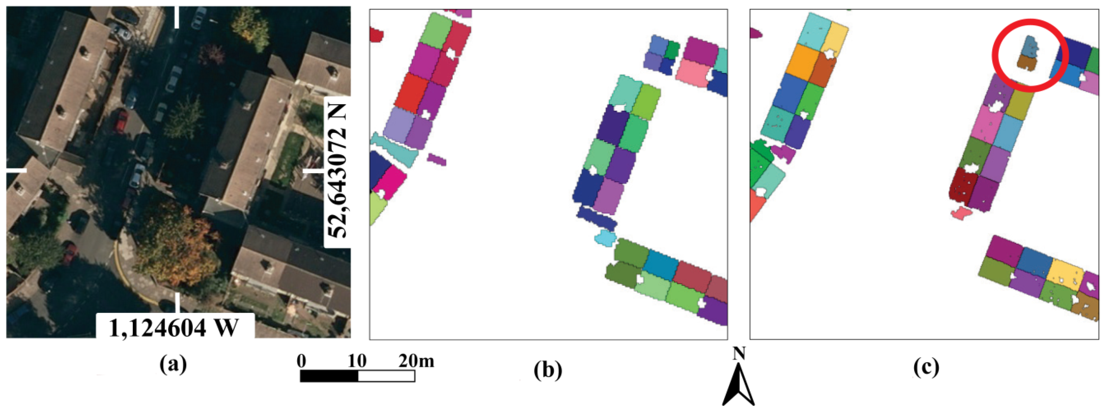
3.2. Roof Plane Extraction

3.2.1. Detection Rates

An example output of the roof plane extraction process can be seen in Figure 5. For each test site, more than 500 roof planes have been selected to determine these quality parameters. The results are sampled in Table 3 and Table 4. For a visual comparison examples of extracted roof planes from both datasets (LiDAR and aerial images) are shown in Figure 8 and Figure 9 for the Leicester and the Karlsruhe test site, respectively.

Table 3. Completeness of roof plane extraction for the Leicester and Karlsruhe test site.

Test Site	Data Type	# Planes	Tp	Fn	Completeness
Leicester (UK)	LiDAR Aerial Images	522	485	37	92.9%
		522	456	66	87.4%
Karlsruhe (GER)	LiDAR Aerial Images	502	483	19	96.2%
		502	484	18	96.4%

Table 3. Completeness of roof plane extraction for the Leicester and Karlsruhe test site.

Test Site	Data Type	# Planes	Tp	Fn	Completeness
Leicester (UK)	LiDAR Aerial Images	522	485	37	92.9%
		522	456	66	87.4%
Karlsruhe (GER)	LiDAR Aerial Images	502	483	19	96.2%
		502	484	18	96.4%

Figure 5. Roof planes extracted by the EAGLE approach from LiDAR data of a subset of the Leicester (UK) test site, DSM raster: 0.25 m, Copyright © Bluesky International Ltd. (Leicestershire, UK). Derived from data © Crown copyright and database right 2012 Ordnance Survey licence number 100042840.

Figure 5. Roof planes extracted by the EAGLE approach from LiDAR data of a subset of the Leicester (UK) test site, DSM raster: 0.25 m, Copyright © Bluesky International Ltd. (Leicestershire, UK). Derived from data © Crown copyright and database right 2012 Ordnance Survey licence number 100042840.

Table 4. Correctness and quality of roof plane extraction for the Leicester and Karlsruhe test site.

Test Site	Data Type	# Planes	Tp	Fp	Correctness	Quality
Leicester (UK)	LiDAR Aerial Img.	522	514	8	98.5%	91.9%
		522	515	7	98.7%	87.6%
Karlsruhe (GER)	LiDAR Aerial Img.	502	453	49	90.2%	86.9%
		502	418	84	83.3%	80.4%

Table 4. Correctness and quality of roof plane extraction for the Leicester and Karlsruhe test site.

Test Site	Data Type	# Planes	Tp	Fp	Correctness	Quality
Leicester (UK)	LiDAR Aerial Img.	522	514	8	98.5%	91.9%
		522	515	7	98.7%	87.6%
Karlsruhe (GER)	LiDAR Aerial Img.	502	453	49	90.2%	86.9%
		502	418	84	83.3%	80.4%

3.2.2. Quality of Roof Plane Parameters

In Table 5, Table 6 and Table 7, the results of the determination of differences between reference and extracted planes are sampled. The calculated measures are based on 28 reference planes (Leicester) and 27 reference planes (Karlsruhe) respectively derived from both data types (LiDAR, aerial images).

Table 5. Differences between inclination angle of the extracted roof planes and their corresponding reference planes for both data types and test sites (Leicester = LEIC, Karlsruhe = KA).

Test Site	Inclination Angle (Degree)
	LiDAR				Aerial Image
	Mean	Max	Min	Std. Dev.	Mean	Max	Min	Std. Dev.
LEIC	1.5	3.9	0.02	1.0	1.7	5.6	0.08	1.1
KA	1.6	4.8	0.06	1.4	1.4	4.2	0.06	1.1

Table 5. Differences between inclination angle of the extracted roof planes and their corresponding reference planes for both data types and test sites (Leicester = LEIC, Karlsruhe = KA).

Test Site	Inclination Angle (Degree)
	LiDAR				Aerial Image
	Mean	Max	Min	Std. Dev.	Mean	Max	Min	Std. Dev.
LEIC	1.5	3.9	0.02	1.0	1.7	5.6	0.08	1.1
KA	1.6	4.8	0.06	1.4	1.4	4.2	0.06	1.1

Table 6. Differences between the aspect angle of the extracted roof planes and their corresponding reference planes for both data types and test sites (Leicester = LEIC, Karlsruhe = KA).

Test Site	Aspect Angle (Degree)
	LiDAR				Aerial Image
	Mean	Max	Min	Std. Dev.	Mean	Max	Min	Std. Dev.
LEIC	1.1	5.3	0.10	1.3	1.4	6.3	0.05	1.4
KA	0.8	1.9	0.02	0.6	0.6	2.0	0.01	0.6

Table 6. Differences between the aspect angle of the extracted roof planes and their corresponding reference planes for both data types and test sites (Leicester = LEIC, Karlsruhe = KA).

Test Site	Aspect Angle (Degree)
	LiDAR				Aerial Image
	Mean	Max	Min	Std. Dev.	Mean	Max	Min	Std. Dev.
LEIC	1.1	5.3	0.10	1.3	1.4	6.3	0.05	1.4
KA	0.8	1.9	0.02	0.6	0.6	2.0	0.01	0.6

Table 7. Differences between the size of the extracted roof planes and their corresponding reference planes for both data types and test sites (Leicester = LEIC, Karlsruhe = KA).

Test Site	Size (%)
	LiDAR				Aerial Image
	Mean	Max	Min	Std. Dev.	Mean	Max	Min	Std. Dev.
LEIC	11.6	34.7	0.3	10.3	12.3	29.9	0.7	9.1
KA	18.4	34.9	0.4	11.2	13.3	30.4	0.4	8.5

Table 7. Differences between the size of the extracted roof planes and their corresponding reference planes for both data types and test sites (Leicester = LEIC, Karlsruhe = KA).

Test Site	Size (%)
	LiDAR				Aerial Image
	Mean	Max	Min	Std. Dev.	Mean	Max	Min	Std. Dev.
LEIC	11.6	34.7	0.3	10.3	12.3	29.9	0.7	9.1
KA	18.4	34.9	0.4	11.2	13.3	30.4	0.4	8.5

Due to the fact that the reference data also possess a degree of inaccuracy (approx. ±0.05 m in positioning, ±0.15 m in height), the mean and maximum differences should be determined, e.g., to recognize gross errors. Since differences in the plane sizes occur mainly at the borders of the roof planes, they depend highly on the size itself, i.e., larger areas understandably cause larger absolute differences in (m²) than smaller areas. Therefore, the differences of plane sizes are given as a percentage (%) of overlap.

3.2.3. Additional Influences on the Quality of the Extracted Roof Planes

The results of DSM generation derived from different image resolutions are depicted in Figure 6. As can clearly be seen, the resolution of 0.20 m pixel size causes significant irregularities even in areas of planar roofs. These undulations in height are of an order of magnitude of 0.3–0.4 m while they are below 0.15 m in the case of 0.06 m pixel size. In the first case, these large deviations from the related roof planes lead to gaps in the extracted areas and larger differences of the geometric plane parameters. From the scientific point of view, more investigations have to be carried out with several resolutions and a minimum of two independent test sites in Europe before reliable results can be presented.

To get a better impression of the influence of image resolution, an example of a DSM derived from an UAV flight with a very high image resolution of 0.02 m pixel size is shown in Figure 7 (but from a different test site in Karlsruhe without ground truth and reference data).

In one case of data acquisition, digital aerial images had been delivered in a compressed data format (jpeg). In a first stage, this dataset was processed in the same manner as all other ones. The resulting DSM showed a significantly worse quality than could be expected from that image resolution. Noticeable undulations inside the roof planes and a higher noise level could be observed. Therefore, a new dataset without compression was ordered which led to the results presented in Section 3.2.1 and Section 3.2.2.

Figure 6. DSMs derived from aerial images of different resolutions (Karlsruhe test site). (a) DSM derived from resolution of 0.20 m; (b) DSM derived from resolution of 0.06 m.

Figure 6. DSMs derived from aerial images of different resolutions (Karlsruhe test site). (a) DSM derived from resolution of 0.20 m; (b) DSM derived from resolution of 0.06 m.

Figure 7. DSM derived from high resolution UAV images: pixel size 0.02 m, flying height approx. 50 m (Karlsruhe test site).

Figure 7. DSM derived from high resolution UAV images: pixel size 0.02 m, flying height approx. 50 m (Karlsruhe test site).

4. Discussion

4.1. Geometric Coincidence of Building Outlines and Building Borders in Height Data (DSM)

The results of this investigation have shown that the displacements between ground truth building outlines and the related building borders in the height datasets are the in the expected range of <1 m (mean difference) and 1.5 m–2 m (max. difference), respectively. These results are in good accordance with other recent publications, e.g., Zeng et al. [37], Troung-Hong and Laefer [39]. These results represent the roof overhangs as well as displacements caused by remaining errors in the navigation data (LiDAR) and exterior orientations (aerial images). Due to the larger roof overhangs in the Karlsruhe test site in comparison to Leicester, it can be observed that almost all maximum gradients lie outside the building polygons. As a consequence for all test sites, a buffer of sufficient size (e.g., 1.5 m or 2.0 m) was placed around the building outlines to extend the processing area for the roof plane extraction. Therefore, the real usable roof areas including overhangs and regarding the mismatches between building outlines and their borders in the DSM data can be determined.

4.2. Roof Plane Extraction

For both test sites, the results derived from LiDAR data concerning detection rates are of the same order of magnitude as other approaches, e.g., Jochem et al. [14], Awrangjeb and Fraser [46], Zeng et al. [37], Truong-Hong and Laefer [39], even if no direct comparison can be made due to different input datasets (data types, resolution, accuracy) and processing methods. All image matching algorithms depend on sufficient image textures, therefore, uniform roof materials or dark shadow areas may lead to errors or gaps in the resulting height data. As a consequence, the extraction quality is worse for aerial images from Leicester. This can be explained by the hard shadow areas occurring in these images which mask image texture and make both point detection and point matching in these areas impossible, causing gaps in the derived height data and the extracted roof planes (cf. Figure 8c, marked red circle). In addition, nearby trees partly covering the roof planes may not be penetrated by LiDAR and, therefore, those roof areas may be incomplete or remain undetected (cf. Figure 5, lower right). Due to the extremely high resolution of the aerial images (pixel size = 6 cm) and significantly less shadowing, the quality is improved for the Karlsruhe test site. As a consequence of the permanent updates of cadastral data in most European countries, missing building outlines of new houses are infrequent. The results of this quality assessment confirm that the detection rates of the extracted roof planes are only marginally affected by rasterization (cf. Section 2.1.1).

Figure 8. Extracted roof planes of the Leicester test site. (a) Aerial image; (b) Roof planes extracted from LiDAR DSM; (c) Roof planes extracted from DSM derived from aerial images. Aerial image: copyright © Bluesky International Ltd. (Leicestershire, UK). Derived from data © Crown copyright and database right 2012 Ordnance Survey licence number 100042840.

Figure 8. Extracted roof planes of the Leicester test site. (a) Aerial image; (b) Roof planes extracted from LiDAR DSM; (c) Roof planes extracted from DSM derived from aerial images. Aerial image: copyright © Bluesky International Ltd. (Leicestershire, UK). Derived from data © Crown copyright and database right 2012 Ordnance Survey licence number 100042840.

Inclination and aspect angles show only small mean differences of about 1°–2°, independent of the data type and test site. This is sufficient for this application because the influence of these small differences on the resulting energy yield is only marginal compared to the uncertainties caused by the (statistical) meteorological data (sun radiation per year) or errors in the determination of the sizes of roof planes. Nevertheless, very few outliers with significantly large differences (up to 6°) occur. The latter observation is also reported by other research groups (e.g., Gooding et al. [35], Truong-Hong and Laefer [39]). The differences of the plane sizes are larger for all data types, approximately 12%–13% with the exception of the results for LiDAR at the test site Karlsruhe (18.4%) which affect the resulting energy yield significantly. The main reason for these larger differences can be ascribed to undetected disturbing roof objects, e.g., dormers, chimneys and especially roof windows which are integrated into the surface of the roofs (cf. Figure 8, center). Dependent on the number and sizes of these roof windows and other undetected objects, the extracted plane size may be up to 30% larger than the reference data, in exceptional cases even more. Therefore, the maximum errors (Table 7) are caused by these error sources. In the Karlsruhe test site, the relatively low resolution of the LiDAR DSM (0.5 m raster size, according to approx. 2 pts./m²) makes this problem more significant, because even medium sized chimneys and dormers may be undetectable and lead to those larger differences of 18.4% (cf. Figure 9). Additionally, in aerial images, hard shadow areas and trees partly covering roof areas induce gaps or missing roof parts which directly affect the determination of the plane size (cf. Figure 8c). Therefore, an improved, detailed extraction of disturbing objects, e.g., based on the image information, is one of the main tasks for future development of the system. Again, an influence of rasterization cannot be recognized in the geometric roof plane parameters.

As shown in Figure 6, the available image resolution has an enormous influence on the automatically derived DSM and, therefore, on the quality of the extracted roof areas. The resolution of 0.20 m pixel size causes significant irregularities and undulations of about 0.3 m–0.4 m even in planar roof areas. The same effect can be seen in the examples of Agugiaro et al. [33]. In contrast, the pixel size of 0.06 m is smaller than the tile size (approx. 0.10 m) which leads to a significant image texture and, therefore, to the extraction of relatively smooth roof surfaces (deviations of <0.15 m) where smaller objects can be detected and excluded. A jump in quality can be observed at an image resolution according approximately to the size of the roof elements (e.g., roof tiles). This observation can be confirmed by additional UAV flights. Figure 7 shows the resulting DSM derived from UAV images of 0.02 m pixel size (flying height approx. 50 m). Even smaller details like vent tubes, roof hatches etc. are recognizable. In conclusion, it can be stated that the generation of DSMs adequate for detailed solar energy applications based on aerial images needs sufficiently high resolution data, i.e., pixel sizes smaller than the roof elements (e.g., <0.1 m). In contrast, for LiDAR data, only moderate resolutions of approx. 0.25 m–0.30 m (equivalent to 10–16 pts./m²) are needed to obtain comparable results. Therefore, higher data resolution of aerial images in the future will lead to an increasing usage of automatic image analysis to generate high quality DSM data, an important aspect due to significantly shorter up-date cycles and nationwide coverage. Also, the compression rate of aerial image data leads to an impairment of the derived DSM data. However, due to the fact that only one case occurred, no validated results can be given here. More investigations with a larger number of datasets of different compression rates for the same test site and the same processing conditions have to be carried out first, not least to clarify possible certain effects caused by the matching algorithm itself.

Figure 9. Extracted roof planes of the Karlsruhe test site. (a) Aerial image; (b) Roof planes extracted form LiDAR DSM; (c) Roof planes extracted from DSM derived from aerial images. Copyright: Datengrundlage © Stadt Karlsruhe, Liegenschaftsamt.

Figure 9. Extracted roof planes of the Karlsruhe test site. (a) Aerial image; (b) Roof planes extracted form LiDAR DSM; (c) Roof planes extracted from DSM derived from aerial images. Copyright: Datengrundlage © Stadt Karlsruhe, Liegenschaftsamt.

4.3. Qualitative Comparison of Results Derived from LiDAR and Aerial Imagery

The final stage of this quality assessment involves a comparison of the results obtained from the two alternative data types: LiDAR and aerial imagery. As Oude Elberink [4] has stated, although there are several problems analyzing LiDAR data for modeling of buildings, the potential of automatic reconstruction in complex scenes is lower when using aerial images. Our investigations for the most part confirm this statement. The automatic generation of a DSM for extracting roof planes from images has a number of disadvantages when compared to LiDAR data.

To obtain DSM of sufficient quality, a high degree of image overlap is necessary. The commonly used overlaps of 60% along-track and 20%–25% across-track are not sufficient in most cases. Our experience has shown that the degree of overlap should be ≥80% along-track and ≥50% across-track. Even if aerial images with such a high degree of overlap are available, vegetation is still impenetrable. In contrast to LiDAR data, roof parts covered by nearby trees are—in most cases—excluded by plane extraction algorithms and roof planes remain incomplete or missed.

Another significant drawback is that automatic image matching methods depend to a large degree on sufficient image texture (significant gradients in different directions) to perform image correlation. There are two sources of homogenous, unstructured areas. First, there are those areas with the same uniform material, e.g., building roofs. Second, there are those hard shadow areas where often no significant points and their point correspondences in the other images can be found, resulting in gaps in the DSM. This may also lead to undesirable inhomogeneous, irregular point distributions and gaps in the extracted object surfaces (Figure 8c).

In contrast to LiDAR data, a further challenge for image matching approaches are the sharp 3D object edges at building borders and roof ridges which appear relatively smooth in the resulting DSM data derived automatically from aerial images. Therefore, the extraction of roof plane borders contains uncertainties largely affecting the determination of their size. As stated in Section 4.2, to achieve reliable results, a very high image resolution is indispensable which may be realized at a nationwide level in the near future.

The disadvantages of LiDAR data—especially for large area datasets—may be the low or medium point densities of 1–4 pts./m² of commonly available large-area datasets while an acceptable quality of roof plane extraction (including the detection of disturbing roof objects) can be obtained from a value of approximately 10–16 pts./m². Another drawback is the lack of multi-spectral information which can be used for an improved detection of building areas. However, the most important disadvantages are the long or undefined up-date cycles as well as an incomplete coverage in most European countries. Therefore, in future, the use of very high resolution aerial imagery for automatic generation of DSM will be significant.

5. Conclusions

A comprehensive quality evaluation of a system for extraction of suitable roof planes for solar energy installations based on the significant factors such as positional displacements, inclination angle, aspect angle, size and additional effects (data resolution, compression rate) was presented. Due to the variable data availability in Europe, we explored the use of alternative input data types in the system workflow (LiDAR data, aerial images). The system is targeted towards two main user groups: on the one hand, individual users like house owners, installers etc., and, on the other hand, governments or solar energy companies interested in large regional areas which must be manageable. The extended quality assessment has proved the benefit of the results obtained based on commonly available datasets: completeness values of about 87%–96%, correctness of about 83%–99% and quality of 80%–92%, mean differences of incidence angles of approximately 1.5°, aspect angles of approximately 1° and a plane size of 14% on average. Additionally, the influence of new quality parameters (image resolution, data compression rate) on the results has been discussed.

Based on higher resolution data, future developments should aim towards a robust process of detection of disturbing roof objects, one of the main error sources in the determination of usable roof areas for solar energy systems. Additional research has to be carried out concerning the influences of image resolution and compression rate on the extracted roof planes as well as the potential of full waveform and multispectral laser sensors (e.g., Slota [47], Yan et al. [48]). An over-detailed calculation algorithm of the subsequent energy yield seems to be questionable due to the fact that such solar potential systems are oriented towards the estimation of energy yield in the future where the enormous variability of annual solar radiation will affect the results much more than the consideration of some details in the calculation algorithm. Another more user-orientated aspect is an easy to use and intuitive web portal for widespread utilization of such a system. In this context, the EAGLE platform [1] will contribute to the increasing dissemination of renewable energy systems in Europe.

References

1. EAGLE Development and Demonstration of a Dynamic, Web-Based, Renewable Energy Rating Platform. Available online: http://www.eagle-fp7.eu (accessed on 28 November 2014).
2. Dorninger, P.; Pfeifer, N. A comprehensive automated 3D approach for building extraction, reconstruction, and regularization from airborne laser scanning point clouds. Sensors 2008, 8, 7323–7343. [Google Scholar] [CrossRef]
3. Noronha, S.; Nevatia, R. Detection and modeling of buildings from multiple aerial images. IEEE Trans. Pattern Anal. Mach. Intell. 2001, 23, 501–518. [Google Scholar] [CrossRef]
4. Oude Elberink, S.J. Problems in automated building reconstruction based on dense airborne laser scanning data. Int. Arch. Photogramm. Remote Sens. Spat. Inf. Sci. 2008, 37, 93–98. [Google Scholar]
5. Vosselman, G.; Maas, H.-G. (Eds.) Airborne and Terrestrial Laser Scanning; Whittles: Dunbeath, UK, 2010.
6. Tarsha-Kurdi, F.; Landes, T.; Grussenmeyer, P. Joint combination of point cloud and DSM for 3D building reconstruction using airborne laser scanner data. In Proceedings of the Urban Remote Sensing Joint Event, Paris, France, 11–13 April 2007.
7. Tarsha-Kurdi, F.; Landes, T.; Grussenmeyer, P.; Koehl, M. Model-driven and data-driven approaches using LiDAR data: Analysis and comparison. Int. Arch. Photogramm. Remote Sens. Spat. Inf. Sci. 2007, 36, 87–92. [Google Scholar]
8. Weidner, U.; Foerstner, W. Towards automatic building extraction from high resolution digital elevation models. ISPRS J. Photogramm. Remote Sens. 1995, 59, 38–49. [Google Scholar] [CrossRef]
9. Maas, H.-G.; Vosselman, G. Two algorithms for extracting building models from raw laser altimetry data. ISPRS J. Photogramm. Remote Sens. 1999, 54, 153–163. [Google Scholar] [CrossRef]
10. Jochem, A.; Hoefle, B.; Hollaus, M.; Rutzinger, M. Object detection in airborne LiDAR data for improved solar radiation modeling in urban areas. Int. Arch. Photogramm. Remote Sens. Spat. Inf. Sci. 2009, 38, W8. [Google Scholar]
11. Schwalbe, E.; Maas, H.-G.; Seidel, F. 3D building model generation from airborne laser scanner data using 2D GIS data and orthogonal point cloud projections. In Proceedings of the ISPRS Workshop Laser Scanning 2005 WG III/3–III/4, Enschede, The Netherlands, 12–14 September 2005.
12. Tarsha-Kurdi, F.; Landes, T.; Grussenmeyer, P. Hough-transform and extended RANSAC algorithms for automatic detection of 3D building roof planes from LiDAR data. In Proceedings of the ISPRS Workshop on Laser Scanning 2007 and SilviLaser 2007, Espoo, Finland, 12–14 September 2007; pp. 407–412.
13. Rottensteiner, F.; Trinder, J.; Clode, S.; Kubik, K. Automated delineation of roof planes from LiDAR data. Int. Arch. Photogramm. Remote Sens. Spat. Inf. Sci. 2005, 36, 221–226. [Google Scholar]
14. Jochem, A.; Hoefle, B.; Rutzinger, M.; Pfeifer, N. Automatic roof plane detection and analysis in airborne LiDAR point clouds for solar potential assessment. Sensors 2009, 9, 5241–5262. [Google Scholar] [CrossRef] [PubMed]
15. Oude Elberink, S.; Vosselman, G. Building reconstruction by target based graph matching on incomplete laser data: analysis and limitations. Sensors 2009, 9, 6101–6118. [Google Scholar] [CrossRef] [PubMed]
16. Xiong, B.; Jancosek, M.; Oude Elberink, S.; Vosselman, G. Flexible building primitives for 3D building modeling. ISPRS J. Photogramm. Remote Sens. 2015, 101, 275–290. [Google Scholar] [CrossRef]
17. Perera, S.N.; Nalani, H.A.; Maas, H.-G. An automated method for 3D roof outline generation and regularization in airborne laser scanner data. In Proceedings of the ISPRS Annals of Photogrammetry, Remote Sensing and Spatial Information Sciences, Melbourne, Australia, 25 August–1 September 2012; pp. 281–286.
18. Awrangjeb, M.; Zhang, C.; Fraser, C.S. Automatic extraction of building roofs using LiDAR data and multispectral imagery. ISPRS J. Photogramm. Remote Sens. 2013, 83, 1–18. [Google Scholar] [CrossRef]
19. Rottensteiner, F.; Brise, C. Automatic generation of building models from LiDAR data and the integration of aerial images. In Proceedings of the International Archives of Photogrammetry, Remote Sensing and Spatial Information Sciences, Dresden, Germany, 8–10 October 2003; Volume XXXIV-3/W13.
20. Rottensteiner, F.; Trinder, J.; Clode, S.; Kubik, K. Fusing airborne laser scanner data and aerial imagery for the automatic extraction of buildings in densely built-up areas. Int. Arch. Photogramm. Remote Sens. Spat. Inf. Sci. 2004, 35, 512–517. [Google Scholar]
21. Brenner, C. Building reconstruction from images and laser scanning. Int. J. Appl. Earth Obs. Geoinform. 2005, 6, 187–198. [Google Scholar] [CrossRef]
22. Novacheva, A. Building roof reconstruction from LiDAR data and aerial images through plane extraction and colour edge detection. Int. Arch. Photogramm. Remote Sens. Spat. Inf. Sci. 2008, 37, 53–57. [Google Scholar]
23. Brenner, C.; Haala, N. Fast production of virtual reality city models. Int. Arch. Photogramm. Remote Sens. Spat. Inf. Sci. 1998, 32, 77–84. [Google Scholar]
24. Vosselman, G.; Dijkman, S. 3D building model reconstruction from point clouds and ground plans. Int. Arch. Photogramm. Remote Sens. Spat. Inf. Sci. 2001, 34, 37–44. [Google Scholar]
25. Kaartinen, H.; Hyyppä, J.; Gülch, E.; Vosselman, G.; Hyyppä, H.; Matikainen, L.; Hofmann, A.; Mäder, U.; Persson, A.; Söderman, U.; et al. Accuracy of 3D city models: EuroSDR comparison. Int. Arch. Photogramm. Remote Sens. Spat. Inf. Sci. 2005, 36, 227–232. [Google Scholar]
26. ISPRS Test Project on Urban Classification and 3D Building Reconstruction: Results. 2013. Available online: http://www2.isprs.org/commissions/comm3/wg4/results.html (accessed on 22 October 2014).
27. Šúri, M.; Hofierka, J. A new GIS-based solar radiation model and its application to photovoltaic assessments. Trans. GIS 2004, 8, 175–190. [Google Scholar] [CrossRef]
28. Wittman, H.; Bajons, P.; Doneus, M.; Friesinger, H. Identification of roof areas suited for solar energy conversion systems. Renew. Energy 1997, 11, 25–36. [Google Scholar] [CrossRef]
29. Voegtle, T.; Steinle, E.; Tovari, D. Airborne laser scanning data for determination of suitable areas for photovoltaics. Int. Arch. Photogramm. Remote Sens. Spat. Inf. Sci. 2005, 36, 215–220. [Google Scholar]
30. Kassner, R.; Koppe, W.; Schüttenberg, T.; Bareth, G. Analysis of the solar potential of roofs by using official LiDAR data. Int. Arch. Photogramm. Remote Sens. Spat. Inf. Sci. 2008, 37, 399–403. [Google Scholar]
31. Edelsbrunner, H.; Kirkpatrick, D.; Seidel, R. On the shape of a set of points in the plane. IEEE Trans. Inform. Theory 1983, 29, 551–559. [Google Scholar] [CrossRef]
32. Ludwig, D.; Lanig, S.; Klärle, M. Location analysis for solar panels by LiDAR-data with geoprocessing—SUN-AREA. In Proceedings of the 23rd International Conference on Informatics for Environmental Protection, Berlin, Germany, 9–11 September 2009; pp. 83–89.
33. Agugiaro, G.; Remondino, F.; Stevanato, G.; de Filippi, R.; Furlanello, C. Estimation of solar radiation on building roofs in mountainous areas. Int. Arch. Photogramm. Remote Sens. Spat. Inf. Sci. 2011, 38, 155–160. [Google Scholar] [CrossRef]
34. Agugiaro, G.; Nex, F.; Remondino, F.; de Filippi, R.; Droghetti, S.; Furlanello, C. Solar radiation estimation on building roofs and web-based solar cadaster. ISPRS Ann. Photogramm. Remote Sens. Spat. Inf. Sci. 2012, 1, 177–182. [Google Scholar] [CrossRef]
35. Gooding, J.; Crook, R.; Tomlin, A.S. Modelling of roof geometries from low-resolution LiDAR data for city-scale solar energy applications using a neighbouring buildings method. Appl. Energy 2015, 148, 93–104. [Google Scholar] [CrossRef]
36. Foody, G. Status of land cover classification accuracy assessment. Remote Sens. Environ. 2002, 80, 185–201. [Google Scholar] [CrossRef]
37. Zeng, C.; Wang, J.; Lehrbass, B. An evaluation system for building footprint extraction from remotely sensed data. IEEE J. Sel. Top. Appl. Earth Observ. Remote Sens. 2013, 6, 1640–1652. [Google Scholar] [CrossRef]
38. Rutzinger, M.; Rottensteiner, F.; Pfeifer, N. A comparison of evaluation techniques for building extraction from airborne laser scanning. IEEE J. Sel. Top. Appl. Earth Observ. Remote Sens. 2009, 2, 11–20. [Google Scholar] [CrossRef]
39. Truong-Hong, L.; Laefer, D.F. Quantitative evaluation strategies for urban 3D model generation from remote sensing data. Comput. Graphics 2015, 49, 82–91. [Google Scholar] [CrossRef]
40. Song, W.; Haithcoat, T.L. Development of comprehensive accuracy assessment indexes for building footprint extraction. IEEE Trans. Geosci. Remote Sens. 2005, 43, 402–404. [Google Scholar] [CrossRef]
41. Fisher, P.F.; Tate, N.J. Causes and consequences of error in digital elevation models. Prog. Phys. Geog. 2006, 30, 467–489. [Google Scholar] [CrossRef]
42. Schuffert, S. An automatic data driven approach to derive photovoltaic-suitable roof surfaces from ALS data. In Proceedings of the Joint Urban Remote Sensing Event (JURSE), Sao Paulo, Brazil, 21–23 April 2013; pp. 267–270.
43. Douglas, D.H.; Peucker, T.K. Algorithms for the reduction of the number of points required to represent a digitized line or its caricature. Can. Cartogr. 1973, 10, 112–122. [Google Scholar] [CrossRef]
44. Meeus, J. Astronomische Algorithmen, 2nd ed.; Johann Ambrosius Barth: Leipzig, Germany, 1994. [Google Scholar]
45. MicMac, IGN. Available online: http://logiciels.ign.fr/?Micmac (accessed on 13 November 2014).
46. Awrangjeb, M.; Fraser, C. Automatic and threshold-free evaluation of 3D building roof reconstruction techniques. In Proceedings of the 2013 IEEE International Geoscience and Remote Sensing Symposium (IGARSS), Melbourne, Australia, 21–26 July 2013; pp. 3970–3973.
47. Slota, M. Full-waveform data for building roof step edge localization. ISPRS J. Photogramm. Remote Sens. 2015, 106, 129–144. [Google Scholar] [CrossRef]
48. Yan, W.Y.; Shaker, A.; El-Ashmawy, N. Urban land cover classification using airborne LiDAR data: A review. Remote Sens. Environ. 2015, 158, 295–310. [Google Scholar] [CrossRef]