
A Comparison of the Performance of Bias-Corrected RSMs and RFMs for the Geo-Positioning of High-Resolution Satellite Stereo Imagery


Abstract
:
1. Introduction
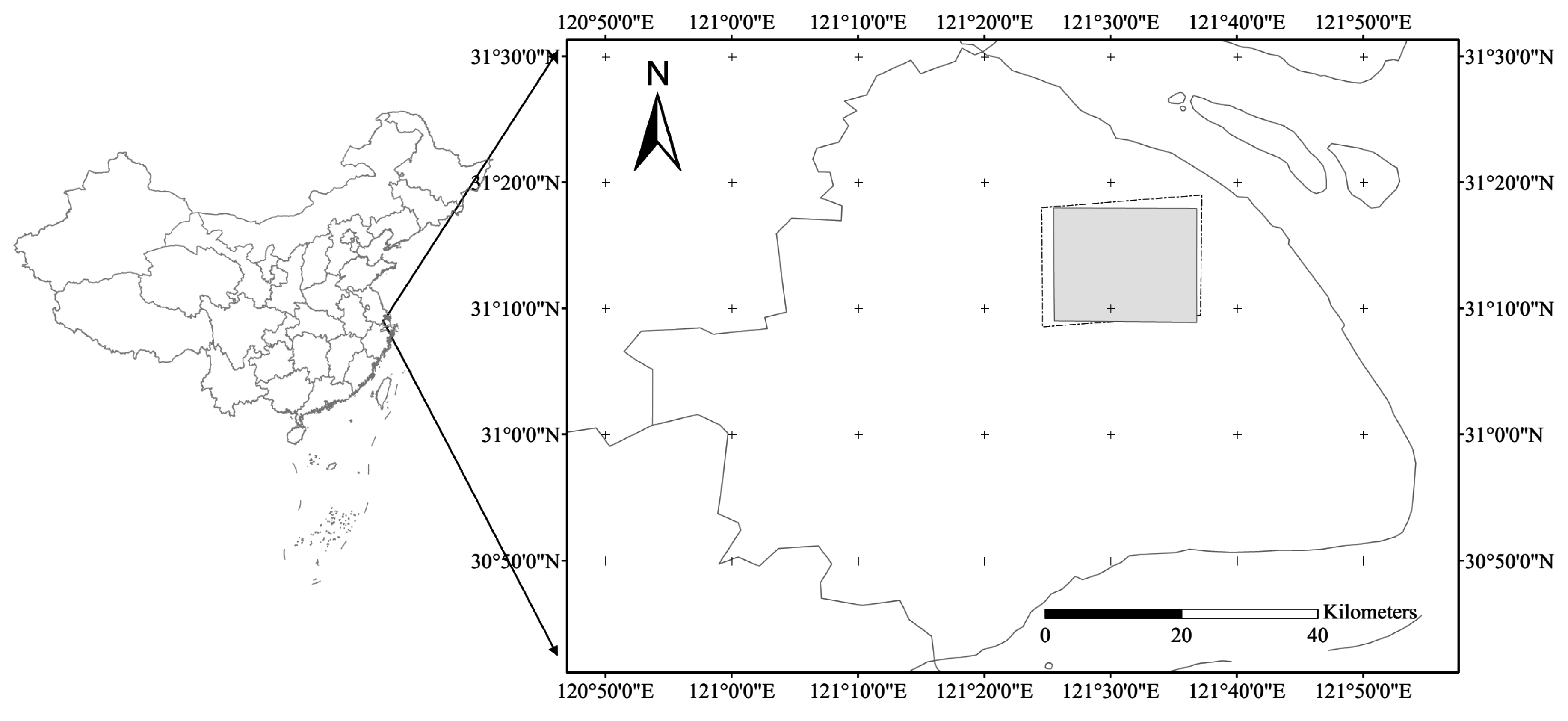
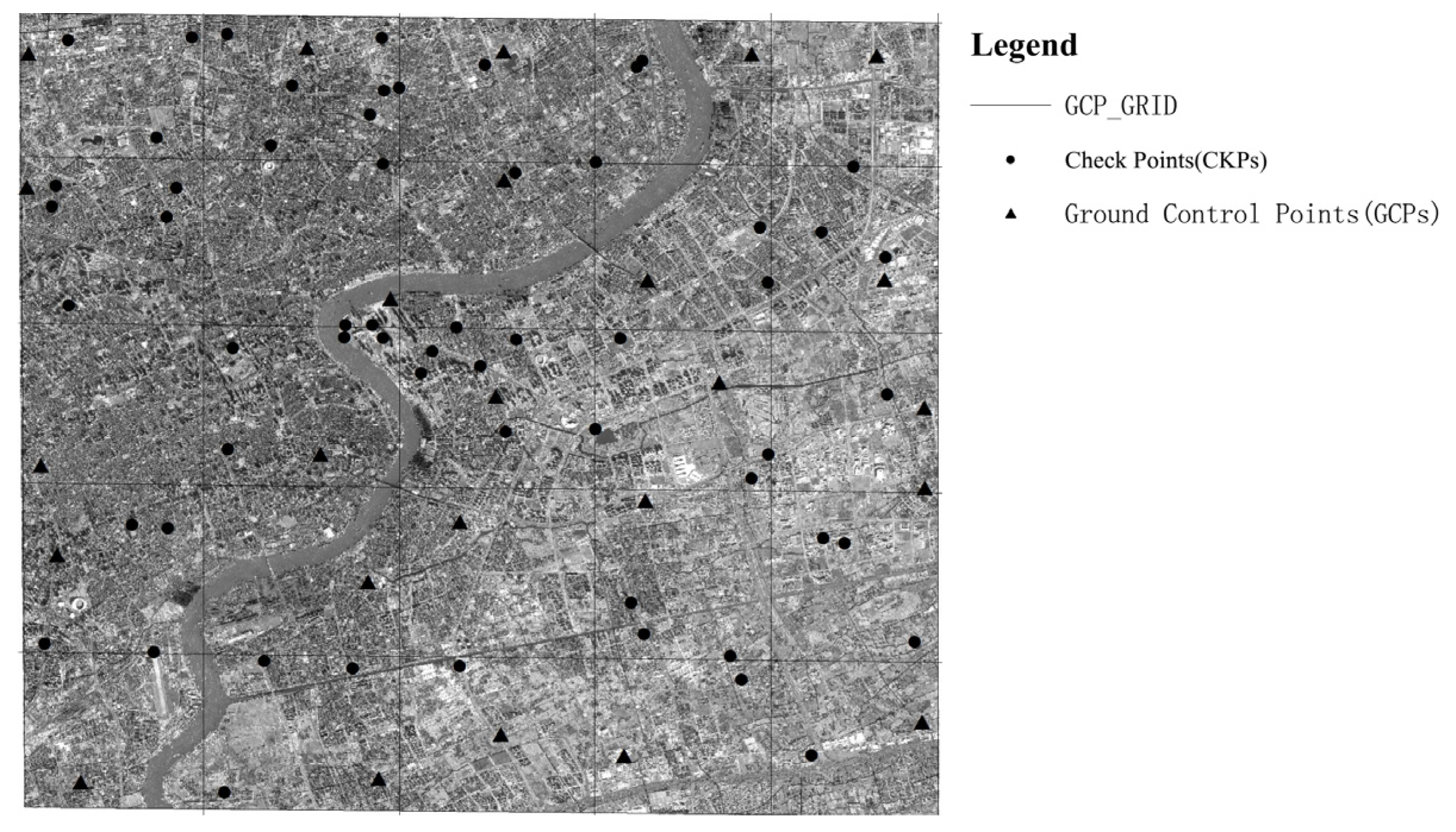
2. Study Area and Data Sources


| Image Information | Left Image Of The Stereo Pair | Right Image of the Stereo Pair |
|---|---|---|
| Acquisition time | 2004-02-15 UTC | 2004-05-05 UTC |
| Scan direction | Forward | Forward |
| Along-track view angle (°) | 19.800 | 14.600 |
| Cross-track view angle (°) | −5.500 | 19.600 |
| Off-nadir view angle (°) | 20.600 | 24.400 |
| Elevation angle (°) | 64.000 | 68.200 |
| Percent cloud cover (%) | 0.000 | 0.000 |
| Spatial resolution (m) | 0.676 | 0.708 |
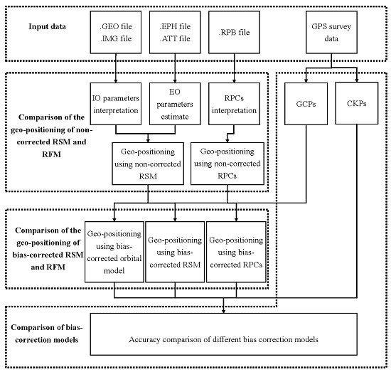
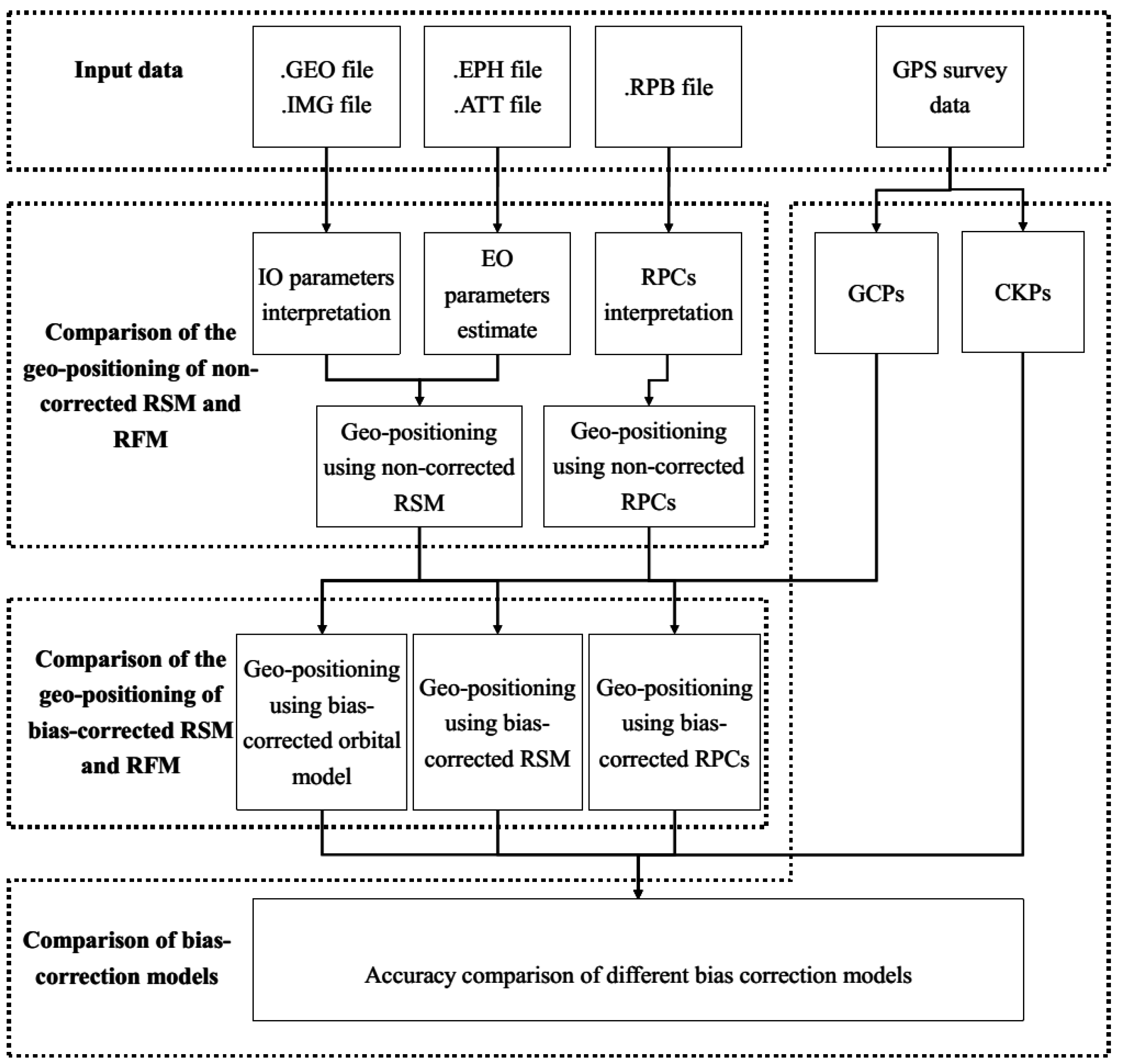
3. Framework

3.1. Geo-Positioning of the Non-Corrected RSM and RFM
3.1.1. Geo-Positioning of the Non-Corrected RSM
3.1.2. Geo-Positioning of the Non-Corrected RFM
3.2. Geo-Positioning of the Bias-Corrected RSM and RFM
4. Results and Analysis
4.1. Results of Geo-Positioning Accuracy of Non-Corrected RSM and RFM
| Model | Number of GCPs/CKPs | Maximum Difference (m) | RMS Error (m) | ||||
|---|---|---|---|---|---|---|---|
| Latitude | Longitude | Height | Latitude | Longitude | Height | ||
| RSM | 0/84 | 13.366 | 27.555 | 20.936 | 12.398 | 21.158 | 15.295 |
| RFM | 0/84 | 13.604 | 27.543 | 21.927 | 12.524 | 21.186 | 16.300 |
4.2. Results of Geo-Positioning Accuracy of Bias-Corrected RSM and RFM
4.2.1. Scenario One, results of Geo-Positioning Accuracy of Bias-Corrected RSM in Orbital Space
| Correction Model | Number of GCPs/CKPs | Maximum Difference between the Measured Coordinates and the Calculated Coordinates of the CKPs (m) | RMS Error of the CKPs (m) | ||||
|---|---|---|---|---|---|---|---|
| Latitude | Longitude | Height | Latitude | Longitude | Height | ||
| Zero-order polynomial model | 3/81 | 1.932 | 1.452 | 3.712 | 0.645 | 0.483 | 1.353 |
| 4/80 | 1.280 | 1.351 | 3.091 | 0.493 | 0.444 | 1.321 | |
| 5/79 | 1.232 | 1.335 | 3.279 | 0.473 | 0.440 | 1.358 | |
| 6/78 | 1.046 | 1.351 | 3.099 | 0.438 | 0.445 | 1.363 | |
| 9/75 | 1.174 | 1.119 | 2.814 | 0.468 | 0.343 | 1.144 | |
| 13/71 | 0.995 | 0.989 | 2.831 | 0.405 | 0.306 | 1.104 | |
| 25/59 | 1.077 | 0.849 | 2.771 | 0.405 | 0.304 | 0.996 | |
| σ = 3 m | 0.933 | 0.873 | 2.998 | 0.425 | 0.294 | 0.948 | |
| First-order polynomial model | 6/78 | 1.199 | 1.074 | 2.894 | 0.479 | 0.375 | 1.284 |
| 9/75 | 1.184 | 0.945 | 2.729 | 0.528 | 0.325 | 1.024 | |
| 13/71 | 1.155 | 0.884 | 2.719 | 0.455 | 0.315 | 0.986 | |
| 25/59 | 1.090 | 0.802 | 2.432 | 0.432 | 0.321 | 0.840 | |
| σ = 3 m | 0.932 | 0.805 | 2.104 | 0.428 | 0.295 | 0.806 | |
| Second-order Polynomial model | 9/75 | 1.213 | 0.949 | 2.564 | 0.533 | 0.323 | 0.984 |
| 13/71 | 1.164 | 0.885 | 2.738 | 0.490 | 0.330 | 0.983 | |
| 25/59 | 0.987 | 0.793 | 2.078 | 0.445 | 0.322 | 0.788 | |
| σ = 3 m | 1.039 | 0.816 | 2.181 | 0.422 | 0.294 | 0.729 | |
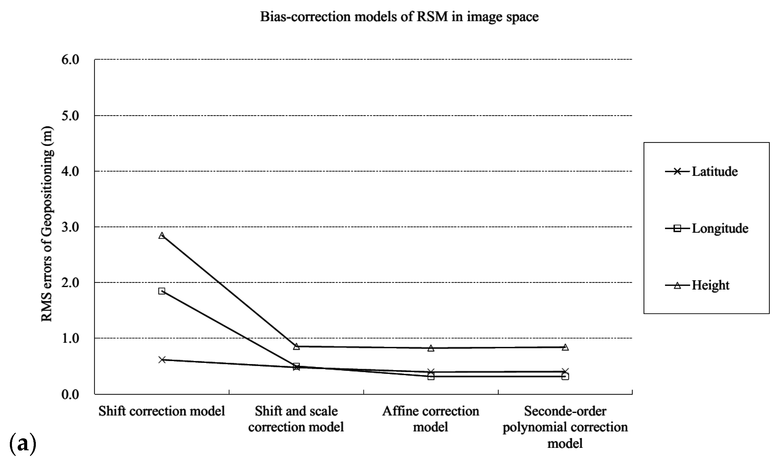
4.2.2. Scenario Two, Results of Geo-Positioning Accuracy of Bias-Corrected RSM in Image Space
| Correction Model | Number of GCPs/CKPs | Maximum Difference between the Measured Coordinates and Calculated Coordinates of the CKPs (m) | RMS Error of the CKPs (m) | ||||
|---|---|---|---|---|---|---|---|
| Latitude | Longitude | Height | Latitude | Longitude | Height | ||
| Shift model | 1/83 | 1.504 | 3.611 | 8.220 | 0.640 | 1.946 | 3.393 |
| 3/81 | 1.342 | 4.298 | 9.407 | 0.680 | 2.160 | 4.130 | |
| 4/80 | 1.349 | 3.436 | 6.575 | 0.690 | 1.894 | 2.876 | |
| 5/79 | 1.303 | 3.470 | 6.356 | 0.673 | 1.909 | 2.951 | |
| 6/78 | 1.328 | 3.585 | 6.591 | 0.665 | 1.937 | 2.910 | |
| 9/75 | 1.355 | 3.580 | 6.653 | 0.660 | 1.907 | 2.885 | |
| 13/71 | 1.446 | 3.578 | 6.447 | 0.623 | 1.931 | 3.000 | |
| 25/59 | 1.416 | 3.324 | 6.047 | 0.618 | 1.851 | 2.849 | |
| σ = 3 m | 1.542 | 3.927 | 7.165 | 0.615 | 1.939 | 2.993 | |
| Shift and scale model | 3/81 | 1.392 | 1.513 | 3.171 | 0.520 | 0.564 | 1.160 |
| 4/80 | 1.310 | 1.453 | 2.933 | 0.561 | 0.524 | 1.181 | |
| 5/79 | 1.261 | 1.416 | 3.166 | 0.543 | 0.520 | 1.188 | |
| 6/78 | 1.247 | 1.343 | 2.855 | 0.536 | 0.508 | 1.184 | |
| 9/75 | 1.206 | 1.268 | 2.416 | 0.529 | 0.490 | 0.995 | |
| 13/71 | 1.293 | 1.264 | 2.533 | 0.496 | 0.501 | 0.950 | |
| 25/59 | 1.251 | 1.017 | 2.540 | 0.482 | 0.502 | 0.859 | |
| σ = 3 m | 1.352 | 1.308 | 2.425 | 0.509 | 0.511 | 0.904 | |
| Affine model | 3/81 | 1.605 | 1.159 | 3.051 | 0.589 | 0.435 | 1.142 |
| 4/80 | 1.252 | 1.158 | 2.741 | 0.500 | 0.416 | 1.225 | |
| 5/79 | 1.200 | 1.109 | 2.961 | 0.479 | 0.407 | 1.229 | |
| 6/78 | 1.255 | 1.134 | 2.826 | 0.503 | 0.392 | 1.251 | |
| 9/75 | 1.174 | 0.985 | 2.593 | 0.476 | 0.337 | 1.055 | |
| 13/71 | 0.999 | 0.910 | 2.588 | 0.413 | 0.318 | 0.984 | |
| 25/59 | 0.934 | 0.821 | 2.428 | 0.398 | 0.319 | 0.828 | |
| σ = 3 m | 0.938 | 0.844 | 2.506 | 0.432 | 0.308 | 0.855 | |
| Second-order polynomial model | 6/78 | 1.970 | 1.991 | 3.555 | 0.854 | 0.716 | 1.617 |
| 9/75 | 0.995 | 1.183 | 2.712 | 0.457 | 0.363 | 1.007 | |
| 13/71 | 0.851 | 1.035 | 2.646 | 0.403 | 0.333 | 0.966 | |
| 25/59 | 0.934 | 0.821 | 2.428 | 0.406 | 0.319 | 0.845 | |
| σ = 3 m | 0.894 | 0.839 | 1.923 | 0.367 | 0.301 | 0.811 | |
4.2.3. Scenario Three, Results of Geo-Positioning Accuracy of Bias-Corrected RFM in Image Space
| Correction Model | Number of GCPs/CKPs | Maximum Difference between the Measured Coordinates and the Calculated Coordinates of the CKPs (m) | RMS Error of CKPs (m) | ||||
|---|---|---|---|---|---|---|---|
| Latitude | Longitude | Height | Latitude | Longitude | Height | ||
| Shift model | 1/83 | 1.696 | 4.032 | 7.175 | 0.607 | 2.231 | 3.151 |
| 3/81 | 1.359 | 4.810 | 9.588 | 0.668 | 2.452 | 4.434 | |
| 4/80 | 1.345 | 3.853 | 6.350 | 0.673 | 2.125 | 2.981 | |
| 5/79 | 1.223 | 3.881 | 6.366 | 0.612 | 2.144 | 2.993 | |
| 6/78 | 1.137 | 3.969 | 6.835 | 0.548 | 2.174 | 2.877 | |
| 9/75 | 1.147 | 3.989 | 6.767 | 0.593 | 2.143 | 2.878 | |
| 13/71 | 1.120 | 3.975 | 6.661 | 0.557 | 2.171 | 2.965 | |
| 25/59 | 1.089 | 3.842 | 6.231 | 0.560 | 2.082 | 2.910 | |
| σ = 3 m | 1.440 | 4.063 | 7.321 | 0.554 | 2.173 | 2.991 | |
| Shift and scale model | 3/81 | 1.306 | 1.479 | 3.855 | 0.484 | 0.556 | 1.487 |
| 4/80 | 1.268 | 1.411 | 3.413 | 0.560 | 0.516 | 1.302 | |
| 5/79 | 1.150 | 1.364 | 3.411 | 0.499 | 0.513 | 1.309 | |
| 6/78 | 0.990 | 1.312 | 2.805 | 0.448 | 0.506 | 1.279 | |
| 9/75 | 1.076 | 1.215 | 2.738 | 0.483 | 0.485 | 1.070 | |
| 13/71 | 0.973 | 1.229 | 2.768 | 0.452 | 0.495 | 1.060 | |
| 25/59 | 0.947 | 1.016 | 2.750 | 0.439 | 0.507 | 0.924 | |
| σ = 3 m | 1.054 | 1.204 | 2.600 | 0.464 | 0.509 | 0.984 | |
| Affine model | 3/81 | 1.532 | 1.156 | 4.067 | 0.543 | 0.476 | 1.459 |
| 4/80 | 1.147 | 1.207 | 3.663 | 0.524 | 0.446 | 1.363 | |
| 5/79 | 1.026 | 1.265 | 3.650 | 0.459 | 0.442 | 1.369 | |
| 6/78 | 0.962 | 1.320 | 2.988 | 0.409 | 0.436 | 1.353 | |
| 9/75 | 1.019 | 1.173 | 2.829 | 0.448 | 0.369 | 1.114 | |
| 13/71 | 0.945 | 1.092 | 2.815 | 0.405 | 0.349 | 1.092 | |
| 25/59 | 0.866 | 0.964 | 2.787 | 0.389 | 0.345 | 0.945 | |
| σ = 3 m | 0.990 | 0.922 | 2.976 | 0.416 | 0.337 | 0.960 | |
| Second-order polynomial model | 6/78 | 3.461 | 4.113 | 4.068 | 1.642 | 1.969 | 1.371 |
| 9/75 | 0.983 | 1.381 | 2.518 | 0.403 | 0.400 | 0.973 | |
| 13/71 | 1.055 | 1.213 | 2.455 | 0.370 | 0.362 | 0.918 | |
| 25/59 | 1.029 | 0.976 | 2.157 | 0.376 | 0.347 | 0.749 | |
| σ = 3 m | 0.967 | 0.919 | 2.221 | 0.346 | 0.328 | 0.777 | |
4.2.4. Scenario Four, Results of Geo-Positioning Accuracy of Bias-Corrected RSM in Object Space
| Correction Model | Number of GCPs/CKPs | Maximum Difference between the Measured Coordinates and the Calculated Coordinates of the CKPs (m) | RMS Error of CKPs (m) | ||||
|---|---|---|---|---|---|---|---|
| Latitude | Longitude | Height | Latitude | Longitude | Height | ||
| Shift model | 1/83 | 1.497 | 4.072 | 7.745 | 0.619 | 2.138 | 3.386 |
| 3/81 | 1.355 | 4.784 | 8.866 | 0.666 | 2.329 | 4.022 | |
| 4/80 | 1.334 | 3.889 | 6.724 | 0.665 | 2.047 | 2.787 | |
| 5/79 | 1.294 | 3.914 | 6.504 | 0.653 | 2.063 | 2.859 | |
| 6/78 | 1.288 | 4.047 | 6.692 | 0.652 | 2.095 | 2.828 | |
| 9/75 | 1.261 | 4.014 | 6.797 | 0.644 | 2.056 | 2.787 | |
| 13/71 | 1.342 | 3.998 | 6.597 | 0.614 | 2.080 | 2.897 | |
| 25/59 | 1.318 | 3.592 | 5.629 | 0.615 | 1.993 | 2.823 | |
| σ = 3 m | 1.573 | 3.995 | 7.303 | 0.612 | 1.914 | 2.918 | |
| Shift and scale model | 3/81 | 1.514 | 1.779 | 3.509 | 0.544 | 0.701 | 1.280 |
| 4/80 | 1.287 | 1.692 | 3.257 | 0.571 | 0.646 | 1.311 | |
| 5/79 | 1.250 | 1.657 | 3.494 | 0.560 | 0.645 | 1.318 | |
| 6/78 | 1.274 | 1.578 | 3.170 | 0.555 | 0.635 | 1.329 | |
| 9/75 | 1.295 | 1.519 | 2.778 | 0.552 | 0.620 | 1.142 | |
| 13/71 | 1.361 | 1.521 | 2.893 | 0.522 | 0.635 | 1.098 | |
| 25/59 | 1.326 | 1.298 | 2.910 | 0.520 | 0.646 | 1.057 | |
| σ = 3 m | 1.424 | 1.351 | 2.617 | 0.529 | 0.594 | 1.034 | |
| Affine model | 4/80 | 6.274 | 1.294 | 6.725 | 1.354 | 0.455 | 1.671 |
| 5/79 | 5.875 | 1.254 | 8.772 | 1.281 | 0.462 | 2.027 | |
| 6/78 | 1.733 | 1.498 | 5.004 | 0.574 | 0.464 | 1.472 | |
| 9/75 | 2.146 | 1.548 | 6.783 | 0.619 | 0.427 | 1.678 | |
| 13/71 | 3.560 | 1.932 | 6.140 | 0.839 | 0.514 | 1.565 | |
| 25/59 | 0.951 | 1.191 | 3.208 | 0.406 | 0.412 | 1.011 | |
| σ = 3 m | 0.937 | 0.860 | 2.560 | 0.406 | 0.313 | 0.865 | |
| Second-order polynomial model | 13/71 | inv | inv | inv | inv | inv | inv |
| 25/59 | 5.711 | 8.824 | 30.073 | 1.172 | 1.304 | 5.376 | |
| σ = 3 m | 0.845 | 0.872 | 1.934 | 0.306 | 0.338 | 0.798 | |
4.2.5. Scenario Five, the Results of Geo-Positioning Accuracy of Bias-Corrected RFM in Object Space
| Correction Model | Number of GCPs/CKPs | Maximum Difference between the Measured Coordinates and the Calculated Coordinates of the CKPs (m) | RMS Error of the CKPs (m) | ||||
|---|---|---|---|---|---|---|---|
| Latitude | Longitude | Height | Latitude | Longitude | Height | ||
| Shift model | 1/83 | 1.800 | 4.075 | 6.777 | 0.634 | 2.110 | 3.085 |
| 3/81 | 1.527 | 4.782 | 9.109 | 0.712 | 2.313 | 4.346 | |
| 4/80 | 1.470 | 3.893 | 6.480 | 0.687 | 2.015 | 2.909 | |
| 5/79 | 1.357 | 3.918 | 6.495 | 0.636 | 2.031 | 2.922 | |
| 6/78 | 1.170 | 3.989 | 6.967 | 0.583 | 2.054 | 2.810 | |
| 9/75 | 1.300 | 4.001 | 6.889 | 0.623 | 2.022 | 2.805 | |
| 13/71 | 1.201 | 3.972 | 6.787 | 0.594 | 2.044 | 2.887 | |
| 25/59 | 1.226 | 3.585 | 5.973 | 0.594 | 1.949 | 2.820 | |
| σ = 3 m | 1.592 | 4.088 | 7.438 | 0.594 | 1.882 | 2.937 | |
| Shift and scale model | 3/81 | 1.359 | 1.672 | 4.224 | 0.505 | 0.683 | 1.576 |
| 4/80 | 1.339 | 1.582 | 3.782 | 0.565 | 0.629 | 1.392 | |
| 5/79 | 1.230 | 1.547 | 3.786 | 0.516 | 0.630 | 1.402 | |
| 6/78 | 1.113 | 1.520 | 3.198 | 0.475 | 0.629 | 1.370 | |
| 9/75 | 1.158 | 1.430 | 3.131 | 0.506 | 0.613 | 1.183 | |
| 13/71 | 1.072 | 1.453 | 3.165 | 0.478 | 0.632 | 1.170 | |
| 25/59 | 1.033 | 1.278 | 3.150 | 0.472 | 0.646 | 1.066 | |
| σ = 3 m | 1.093 | 1.328 | 2.915 | 0.485 | 0.594 | 1.091 | |
| Affine model | 4/80 | 4.850 | 1.224 | 6.527 | 1.066 | 0.434 | 1.768 |
| 5/79 | 5.331 | 1.325 | 5.342 | 1.167 | 0.481 | 1.609 | |
| 6/78 | 6.003 | 1.362 | 6.477 | 1.305 | 0.478 | 1.720 | |
| 9/75 | 1.982 | 1.590 | 3.226 | 0.571 | 0.415 | 1.218 | |
| 13/71 | 3.196 | 2.012 | 3.023 | 0.762 | 0.517 | 1.192 | |
| 25/59 | 1.026 | 1.205 | 3.987 | 0.399 | 0.396 | 1.132 | |
| σ = 3 m | 0.866 | 0.902 | 2.965 | 0.379 | 0.301 | 0.959 | |
| Second-order polynomial model | 13/71 | inv | inv | inv | inv | inv | inv |
| 25/59 | 5.875 | 8.422 | 32.980 | 0.990 | 1.314 | 5.349 | |
| σ = 3 m | 0.948 | 0.895 | 2.210 | 0.309 | 0.295 | 0.755 | |
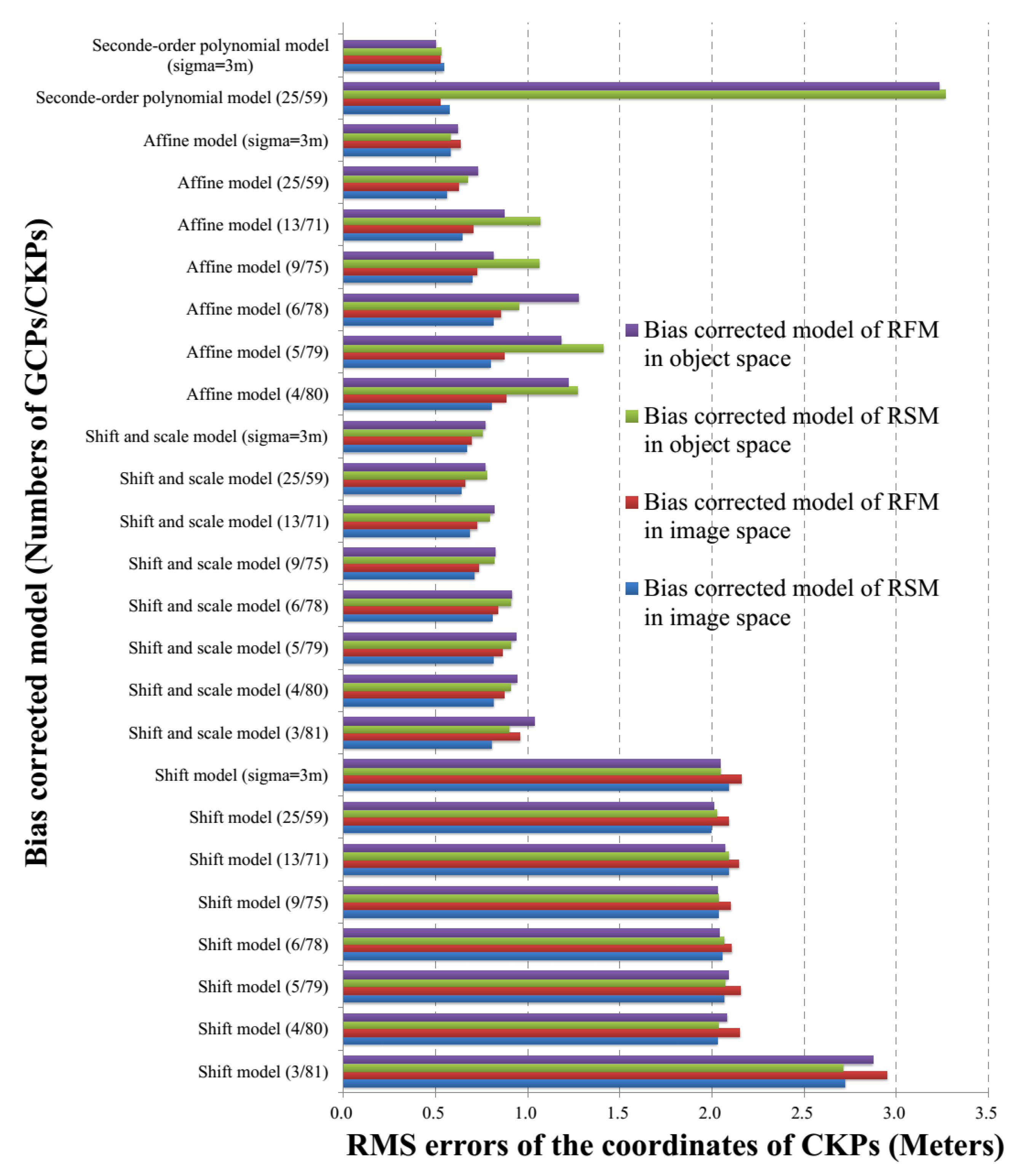
4.3. Comparison and Discussion of the Performance of Bias-Correction Models of the RSM and RFM
4.3.1. Comparison of the Performance of Bias-Correction Models
- (1)
- From the results in Table 3, we can see that all three bias-correction models presented a good performance in geo-positioning accuracy, and second-order polynomial model achieved highest accuracy of 0.5 m in horizontal direction and 0.7 m in vertical direction.
- (2)
- From Table 4, Table 5, Table 6 and Table 7, it can be seen that shift bias-correction model is an efficient model. In Scenarios two to five, the results of geo-positioning accuracy by use of shift bias-correction model with only one GCP show that the geo-positioning accuracy has been greatly improved and reached 2.3 m in horizontal direction and 3.4 m in vertical direction. At the same time, the highest accuracy of 0.7 m in latitude was achieved. However, the accuracy was not greatly improved with an increase in the number of GCPs.
- (3)
- From Table 4, Table 5, Table 6 and Table 7, it can be seen that shift and scale correction model is one of the most stable models in the geo-positioning performance of RSM and RFM in both image and object spaces. By use of three well-distributed GCPs, the geo-positioning achieved sub-pixel accuracy in planimetry. In addition, the geo-positioning accuracy reached 0.5 m in horizontal direction and about 1.0 m in vertical direction as the number of GCPs increased to 25.
- (4)
- From Table 4, Table 5, Table 6 and Table 7, affine bias-correction model achieved the highest accuracy of 0.398 m in latitude, 0.319 m in longitude, and 0.828 m in height with respect to bias-corrected RSM in the image space when the GCPs reached 25 points. However, a poorer performance was observed in the experiments with bias-corrected RSM and RFM in the object space when the number of GCPs was less (for example, three GCPs in Table 6 and four GCPs in Table 7).
- (5)
- From Table 4, Table 5, Table 6 and Table 7, it can be seen that second-order polynomial correction model obtained the highest accuracy of 0.376 m in latitude, 0.347 m in longitude, and 0.749 m in height with respect to bias-corrected RFM in image space when the GCPs reached 25 points. However, the computation did not converge in the experiments with the bias-corrected RSM and RFM in object space when the number of GCPs was 13, as shown in Table 6 and Table 7.
4.3.2. Comparison of the Performance of Bias-Correction Spaces


4.3.3. Comparison of the Performance of Bias-Correction of Geometric Sensor Models

5. Conclusions
- (1)
- By use of zero-order polynomial correction model in orbital space and a minimum of three GCPs, the refined RPCs improved the accuracy to 0.8 m in planimetry and 1.3 m in height, which indicates that the low-order correction model in orbital space can accurately reduce the effects of ephemeris and attitude errors.
- (2)
- The geo-positioning accuracy with RSM was better than that of RFM in both image and object spaces by use of bias correction models, and the low-order correction models (such as affine model, shift and scale model) can achieve a sub-pixel accuracy in horizontal direction with a few number of GCPs (for example, one to three GCPs).
- (3)
- High-order polynomial correction models (such as second-order polynomial model) performed rather unstable, particularly in object space.
Acknowledgments
Author Contributions
Conflicts of Interest
References
- Kim, T.; Dowman, I.J. Comparison of two physical sensor models for satellite images. Photogramm. Rec. 2006, 21, 110–123. [Google Scholar] [CrossRef]
- Poli, D. A rigorous model for spaceborne linear array sensors. Photogramm. Eng. Remote Sens. 2007, 73, 187–196. [Google Scholar] [CrossRef]
- Tao, C.V.; Hu, Y. 3D reconstruction methods based on the rational function model. Photogramm. Eng. Remote Sens. 2002, 68, 705–714. [Google Scholar]
- Di, K.C.; Ma, R.J.; Li, R.X. Geometric processing of Ikonos stereo imagery for coastal mapping applications. Photogramm. Eng. Remote Sens. 2003, 69, 873–879. [Google Scholar]
- Kim, T.; Kim, H.; Rhee, S. Investigation of physical sensor models for modeling SPOT 3 orbits. Photogramm. Rec. 2007, 22, 257–273. [Google Scholar] [CrossRef]
- Weser, T.; Rottensteiner, F.; Willneff, J.; Poon, J.; Fraser, C.S. Development and testing of a generic sensor model for pushbroom satellite imagery. Photogramm. Rec. 2008, 23, 255–274. [Google Scholar] [CrossRef]
- Teo, T.A. Bias Compensation in a Rigorous Sensor Model and Rational Function Model for High-Resolution Satellite Images. Photogramm. Eng. Remote Sens. 2011, 77, 1211–1220. [Google Scholar] [CrossRef]
- Li, R.; Zhou, F.; Niu, X.; Di, K. Integration of Ikonos and QuickBird imagery for geopositioning accuracy analysis. Photogramm. Eng. Remote Sens. 2007, 73, 1067–1074. [Google Scholar]
- Habib, A.; Kim, K.; Shin, S.W.; Kim, C.; Bang, K.I.; Kim, E.M.; Lee, D.C. Comprehensive analysis of sensor modeling alternatives for high-resolution imaging satellites. Photogramm. Eng. Remote Sens. 2003, 73, 1241–1251. [Google Scholar] [CrossRef]
- Li, R.; Niu, X.T.; Liu, C.; Wu, B.; Deshpande, S. Impact of imaging geometry on 3D geopositioning accuracy of stereo IKONOS imagery. Photogramm. Eng. Remote Sens. 2009, 75, 1119–1125. [Google Scholar] [CrossRef]
- Robertson, B. Rigorous geometric modeling and correction of QuickBird imagery. In Proceedings of the 2003 IEEE International Geoscience and Remote Sensing Symposium, Toulouse, France, 21–25 July 2003; pp. 21–25.
- Fraser, C.S.; Hanley, H.B. Bias compensated RPCs for sensor orientation of high-resolution satellite imagery. Photogramm. Eng. Remote Sens. 2005, 71, 909–915. [Google Scholar] [CrossRef]
- Tong, X.H.; Liu, S.J.; Weng, Q.H. Geometric processing of QuickBird stereo imageries for urban land use mapping, a case study in Shanghai, China. IEEE J. Sel. Top. Appl. Earth Obs. Remote Sens. 2009, 2, 61–66. [Google Scholar] [CrossRef]
- Tong, X.H.; Liu, S.J.; Weng, Q.H. Bias-corrected rational polynomial coefficients for high accuracy geo-positioning of QuickBird stereo imagery. ISPRS J. Photogramm. Remote Sens. 2010, 65, 218–226. [Google Scholar] [CrossRef]
- Grodecki, J.; Dial, G. Block adjustment of high-resolution satellite images described by rational polynomials. Photogramm. Eng. Remote Sens. 2003, 69, 59–68. [Google Scholar] [CrossRef]
- Liu, S.; Fraser, C.S.; Zhang, C.; Ravanbakhsh, M.; Tong, X. Georeferencing performance of THEOS satellite imagery. Photogramm. Rec. 2011, 26, 250–262. [Google Scholar] [CrossRef]
- Poli, D.; Toutin, T. Review of developments in geometric modelling for high resolution satellite pushbroom sensors. Photogramm. Rec. 2012, 27, 58–73. [Google Scholar] [CrossRef]
- Zhang, Y.; Wang, B.; Zhang, Z.; Duan, Y.; Zhang, Y.; Sun, M.; Ji, S. Fully automatic generation of geoinformation products with Chinese ZY-3 satellite imagery. Photogramm. Rec. 2014, 29, 383–401. [Google Scholar] [CrossRef]
- Fraser, C.S.; Hanley, H.B. Bias compensation in rational functions for IKONOS satellite imagery. Photogramm. Eng. Remote Sens. 2003, 69, 53–58. [Google Scholar] [CrossRef]
- Noguchi, M.; Fraser, C.S.; Nakamura, T.; Shimono, T.; Oki, S. Accuracy assessment of QuickBird stereo imagery. Photogramm. Rec. 2004, 19, 128–137. [Google Scholar] [CrossRef]
- Orun, A.B.; Natarajan, K. A bundle adjustment software for SPOT imagery and photography, Tradeoff. Photogramm. Eng. Remote Sens. 1994, 60, 1431–1437. [Google Scholar]
- Li, R. Potential of high-resolution satellite imagery for National Mapping Products. Photogramm. Eng. Remote Sens. 1998, 64, 1165–1169. [Google Scholar]
- Toutin, T. Comparison of stereo-extracted DTM from different high-resolution sensors, SPOT-5, EROS-A, IKONOS-II and QuickBird. IEEE Trans. Geosci. Remote Sens. 2004, 42, 2121–2129. [Google Scholar] [CrossRef]
- Tikhonov, A.N.; Arsenin, V.Y. Solutions of Il l-Posed Problems; Wiley: New York, NY, USA, 1977. [Google Scholar]
- DitigalGlobe. QuickBird Imagery Products—Product Guide, Revision 4.7.3; DitigalGlobe, Inc.: Longmont, CO, USA, 2007. [Google Scholar]
- Wang, J.; Di, K.; Li, R. Evaluation and improvement of geopositioning accuracy of IKONOS stereo imagery. J. Surv. Eng. 2005, 13, 35–42. [Google Scholar] [CrossRef]
- Fraser, C.S.; Dial, G.; Grodecki, J. Sensor orientation via RPCs. ISPRS J. Photogramm. Remote Sens. 2006, 60, 182–194. [Google Scholar] [CrossRef]
- Tong, X.H.; Hong, Z.H.; Liu, S.J.; Zhang, X.; Xie, H.; Li, Z.Y.; Yang, S.L.; Wang, W.A.; Bao, F. Building-damage detection using pre- and post-seismic high-resolution IKONOS satellite stereo imagery, a case study of the May 2008 Wenchuan Earthquake. ISPRS J. Photogramm. Remote Sens. 2012, 68, 13–27. [Google Scholar] [CrossRef]
© 2015 by the authors; licensee MDPI, Basel, Switzerland. This article is an open access article distributed under the terms and conditions of the Creative Commons by Attribution (CC-BY) license (http://creativecommons.org/licenses/by/4.0/).
Share and Cite
Hong, Z.; Tong, X.; Liu, S.; Chen, P.; Xie, H.; Jin, Y. A Comparison of the Performance of Bias-Corrected RSMs and RFMs for the Geo-Positioning of High-Resolution Satellite Stereo Imagery. Remote Sens. 2015, 7, 16815-16830. https://doi.org/10.3390/rs71215855
Hong Z, Tong X, Liu S, Chen P, Xie H, Jin Y. A Comparison of the Performance of Bias-Corrected RSMs and RFMs for the Geo-Positioning of High-Resolution Satellite Stereo Imagery. Remote Sensing. 2015; 7(12):16815-16830. https://doi.org/10.3390/rs71215855
Chicago/Turabian StyleHong, Zhonghua, Xiaohua Tong, Shijie Liu, Peng Chen, Huan Xie, and Yanmin Jin. 2015. "A Comparison of the Performance of Bias-Corrected RSMs and RFMs for the Geo-Positioning of High-Resolution Satellite Stereo Imagery" Remote Sensing 7, no. 12: 16815-16830. https://doi.org/10.3390/rs71215855