An Adaptive Method of Wave Spectrum Estimation Using X-Band Nautical Radar

Abstract

In this paper, the dependency of wave spectrum estimation on the analysis window orientation for X-band marine radar data is investigated. The investigation is made for the case where both wind wave and swell components are present. Our results show that more accurate and reliable wave spectrum estimates are obtained when one analysis window for each component (wind waves or swell) is used and is oriented in the up-wave direction of that component. The final wave spectrum estimation is found by averaging the output of those analysis windows. Since the direction of wind waves and swell is not known a priori, a new method is proposed to recursively determine the number and orientation of analysis windows. This method is referred to as the Adaptive Recursive Positioning Method (ARPM). For validation, ocean wave spectra are estimated from X-band marine radar field data using the ARPM and the standard method, using uniformly distributed analysis windows. The results from both methods are compared to ground truth wave spectra acquired using waverider buoy data. Results have shown that the ARPM produces a 10% improvement in the agreement (represented by the correlation coefficient) between the ground truth wave spectrum and the marine radar estimated wave spectrum. This improvement is reflected in a 15% to 30% accuracy enhancement in the wave period estimation and $6^{\circ }$ in peak wave direction. The ARPM not only increases the accuracy of wave period and direction estimation, but it also increases the method’s reliability by producing a lower error standard deviation. Although these improvements are at the price of extra computational time, it has been found that this overhead is acceptable since it is far from the upper bound that requires offline analysis.

1. Introduction

Compared to traditional methods of estimating ocean wave spectra using surface buoys, methods which utilize marine radar may prove to be better in terms of mobility and flexibility. This is basically for two reasons. First, watercraft that have already deployed marine radars are using them for purposes other than sea state estimation, such as target detection. Secondly, a marine radar can be easily focused on any area of the ocean by directing the beam of the shipboard system to that region. This in fact gives a great advantage to this method over the buoy method which can provide only point measurements. Moreover, due to the higher spatial resolution of marine radar images, the spectral shape estimated from marine radar images is smoother, i.e., has a lower variance, than the one from a directional buoy system.

When local wind generates small ripples on the ocean surface, ocean waves become visible to marine radars. This is due to Bragg scattering [1] in which the grazing angle electromagnetic radar pulses interact with those ocean surface ripples which have wavelengths half that of the electromagnetic radar signal. Therefore, at X-band, the surface features give rise to the dominant scatter that have wavelengths on the order of centimeters. Hydrodynamically, the ocean surface ripples are modulated by gravity ocean waves of a much longer wavelength, up to hundreds of metres in some cases [1,2]. The base signal received by the radar is influenced by this ocean surface modulation. In addition to the hydrodynamic modulation, other factors that contribute to the ocean surface backscatter include shadowing and tilt modulation. The shadowing occurs when higher waves hide shorter ones [1,3,4]. In tilt modulation, the strength of the backscattered signal from a certain point on the ocean surface depends on the facet orientation at that point [4]. The radar output, which is modulated by these mechanisms, is referred to as sea clutter and commonly consists of alternating illuminated and shadowed areas forming a strip-like pattern. Traditionally for target detection applications, sea clutter is considered as noise [5]. However, over the last couple of decades, sea clutter has started to be considered as a feature which carries useful information about ocean currents and waves. Radar sea echo is analyzed using methods such as the Cartesian three dimensional (3D) Fourier transformation to produce image spectra. Valuable information about the ocean, including surface current vectors, significant wave height and wave velocity, can be extracted from the image spectra [4,6,7,8,9].

In 1985, Young et al. [6] introduced the idea of using the 3D Cartesian Fourier transformation (CFT) to estimate sea state from X-band nautical radar images. Subsequently, several studies (e.g., [4,9]) were conducted to validate the performance of this method. Moreover, in addition to ocean wave spectrum and surface current estimation [10,11,12,13], this method has been developed further to estimate other sea state parameters or contributing factors such as wind vectors [14,15,16] and bathymetry [17,18]. Many studies in this area have focused on minimizing the sources of error in the original method. For example, several methods have been proposed to enhance the accuracy of surface current estimation which is used to exclude the non-wave spectrum component from the wave spectrum and to calculate the spectrum signal to noise ratio ($SNR$) [11,12,19]. Other studies focused on the Modulation Transfer Function (MTF) which is used to compensate for the distortion presented in the wave spectrum due to the radar imaging process [4,9,20]. However, to date the effects of shadowing and tilt modulation are not completely understood and no generic MTF form has been established yet. Another source of error is the dependency of the returned radar signal strength on the azimuth direction. In the past, this problem has been addressed by averaging the wave spectrum over several analysis windows that are spatially uniformly distributed as shown in Figure 1 [21]. Hereafter in this manuscript, this approach is referred to as the standard method. Except for a study by Lund et al. [22], this problem has not been sufficiently discussed in the literature. In the Lund et al. study, the effect of the analysis window location (range and orientation) is studied in the context of $SNR$. It is also proposed in [22] to choose the orientation of the analysis window in the up-wave direction for maximum $SNR$ which provides, by extension, a better wave spectrum estimation. In this paper, the wave spectrum estimation dependency has been further investigated, particularly in the presence of both types of waves as manifested by wave spectrum components (wind waves and swell). Also, a new adaptive algorithm, referred to as the Adaptive Recursive Positioning Method (ARPM), is proposed to minimize the effect of this dependency. The ARPM works best for radar systems that provide a wide field of view such as offshore platforms and vessels. On the other hand, for limited fields of view, such as may be available for land-based deployments, the ARPM might not provide much improvement over the standard method.

The remainder of this paper is organized as follows. Section 2 contains a review of wave spectrum estimation using marine radar data. An analysis of the dependency of wave spectrum estimation on the analysis window orientation is conducted in Section 3. In Section 4, the new method is presented. Experiment setup and data overview are described in Section 5. Section 6 contains results and analysis. Conclusions and a brief consideration of future work are presented in Section 7.

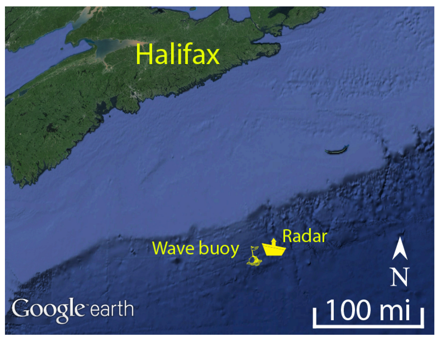
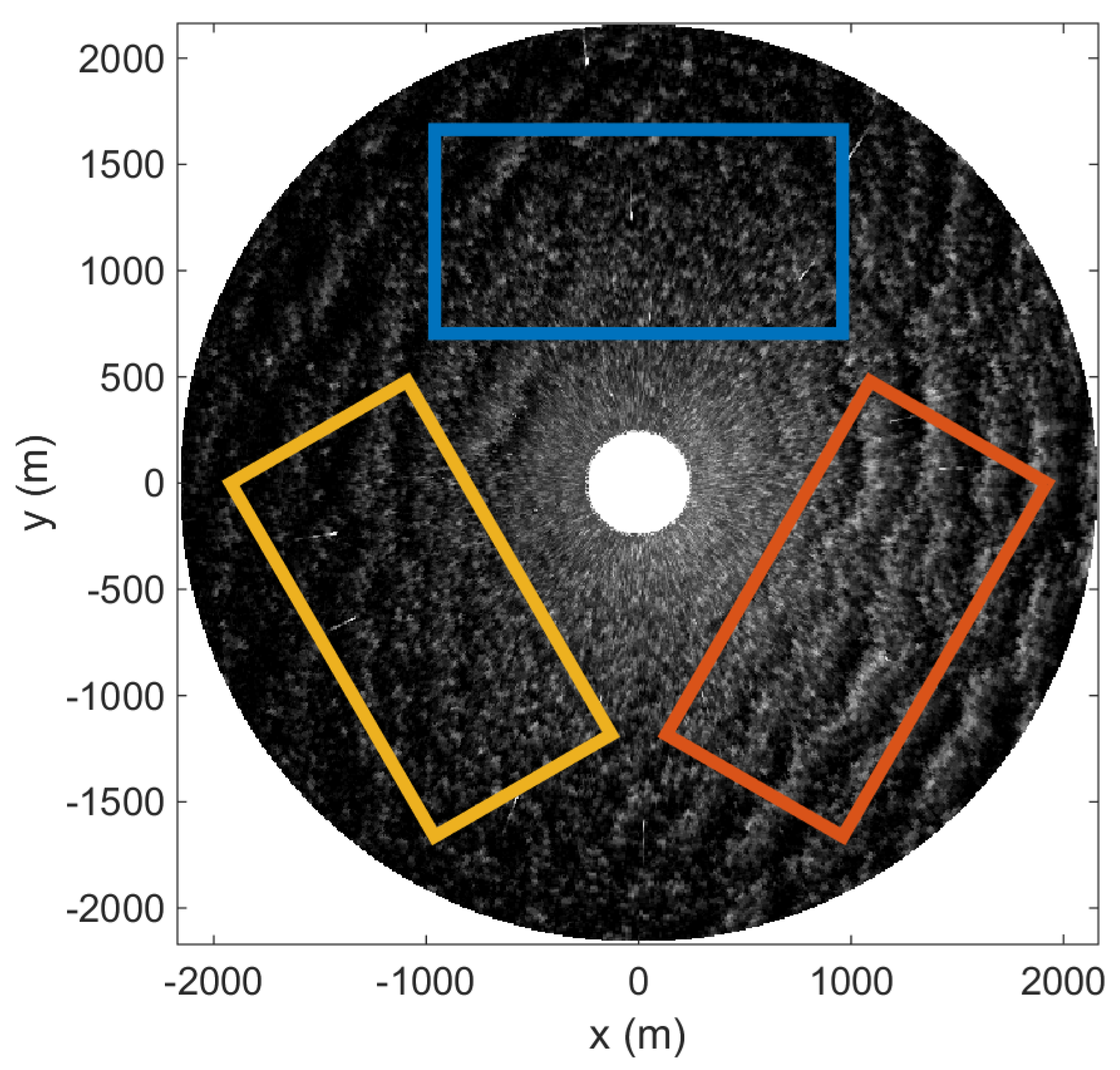
Figure 1. Single scan converted radar image with 3 uniformly distributed analysis windows. 1 December 2008, Atlantic ocean near Halifax.

Figure 1. Single scan converted radar image with 3 uniformly distributed analysis windows. 1 December 2008, Atlantic ocean near Halifax.

2. Review of Wave Spectrum Estimation Using Marine Radar

A typical ocean state measurement by marine radar is obtained from a sequence of sea clutter radar images with a fixed delay time between successive images. This delay time, typically ranging from 1 to 2 s, is basically the rotation time of the radar and depends on the radar design and the experimental setup. Thus, the radar may be used to provide near real-time monitoring of the ocean state. Spatial coverage of the ocean is within the range of several square kilometres and has a range resolution of 1 to 10 metres depending on the radar settings.

The first step is to select an analysis window, $I\left(\xi \right)$, from the Cartesian image sequence, where $\xi =(x,y,t)$ is the space-time vector. Typically, the size of the window is 128 × 128 × 32 or 128 × 256 × 32. In our analysis we use the 128 × 256 × 32 size to cover a wider area in the azimuth dimension which reduces the output dependency on the analysis window orientation. Using a radar resolution of 7.5 m/sample and 1.4 s rotational time, the area-time size of the analysis window is 960 m × 1920 m × 44.8 s. Traditionally, in order to eliminate the dependency on the analysis window orientation, the final wave spectrum estimation is acquired by averaging the wave spectra estimates from multiple analysis windows that are uniformly distributed over the azimuth dimension.

The next step is to apply the 3D Cartesian Fourier Transform (CFT) to $I\left(\xi \right)$ to obtain

$$F(\Omega )=\sum _{j=0}^{N-1}I\left({\xi }_j\right)exp(-i\Omega ·{\xi }_j)$$

(1)

where Ω is the three dimensional wave number-frequency vector ($k_x,k_y,\omega$) with $k_x$ and $k_y$ being the spatial wave vector components and $\omega =2\pi f$ the wave angular frequency. N is the number of points in the discrete space-time vector ξ.

The image spectrum F contains the wave spectrum E and non-wave components coming from noise or aliasing effects. In order to eliminate the non-wave components, a band pass filter with a center angular frequency ${\omega }_e$ is applied, where ${\omega }_e$ is given by the dispersion relationship as

$${\omega }_e(\mathbf{k},\mathbf{U})=\sqrt{g\left|\mathbf{k}\right|tanh\left(\right|\mathbf{k}\left|d\right)}+\mathbf{k}·\mathbf{U}$$

(2)

where $\mathbf{k}=(k_x,k_y)$ is the wave vector of magnitude $\left|\mathbf{k}\right|=2\pi /\lambda ,\lambda$ being the wavelength, in the direction of wave propagation, d the water depth, g the acceleration due to gravity, and $\mathbf{U}$ the velocity of encounter vector which is the sum of the surface current velocity and the radar platform velocity. Unfortunately, $\mathbf{U}$ is unknown. However, several methods have been proposed to estimate it [6,10,11,12,19,23].

Integrating the wave spectrum $E(\Omega )$ over ω yields a wave number spectrum $E_k$ which is a function of ($k_x,k_y$) as given by

$$E_k(k_x,k_y)={\int }_{\omega >0}E(\Omega )\mathrm{d}\omega$$

(3)

Considering only a one-sided interval of frequencies (positive or negative) removes the ambiguity in wave direction which results when the entire range of frequencies ($-\infty <\omega <\infty$) is considered. Subsequently, the frequency-direction spectrum $E(\omega ,\theta )$, commonly known as the directional wave spectrum, can be equivalently represented as

$$E(f,\theta )=E(k_x,k_y)k\frac{\mathrm{d}k}{\mathrm{d}\omega }$$

(4)

where $f=\omega /2\pi$ is the ocean wave frequency, k and θ are the magnitude and angle of k, respectively, and $k\mathrm{d}k/\mathrm{d}\omega$ is the Jacobian between the coordinates ($k_x,k_y$) and ($f,\theta$). The frequency spectrum $S\left(f\right)$ can be given by

$$S\left(f\right)={\int }_{-\pi }^{\pi }E(f,\theta )\mathrm{d}\theta$$

(5)

The $n^{th}$ spectral moment $m_n$ is defined as

$$m_n={\int }_0^{\infty }{f}^{n}S\left(f\right)\mathrm{d}f$$

(6)

The zero-crossing period is given by $T_z={(m_0/m_2)}^{1/2}$, the mean period $T_{01}=m_0/m_1$, and the peak wave period $T_p=1/f_p$ where $f_p$ is the peak frequency [24].

Unfortunately, the significant wave height $H_s$ cannot be estimated directly using the Cartesian Fourier transformation method since the wave spectrum does not reflect the actual ocean wave energy and a calibration process is needed [25]. A recent study proposed a new method using the shadowing in radar images to estimate the significant wave height without the need for calibration [26].

3. The Wave Spectrum Estimation Dependency on the Orientation of the Analysis Window

In wave spectrum estimation using marine radar images, the dependency on the azimuth direction of the analysis window is not a hydrodynamical property of the ocean waves. Rather it is due to the imaging process. Several imaging mechanisms including the intensity variation in the up/down wave direction due to Bragg scattering, shadowing, and tilt modulation contribute to this dependency. The Bragg scattering contribution can be explained by the concentration of the centimeter-scale roughness on the up-wave surface of the wind waves. Since this roughness is responsible for Bragg scattering, it is expected that there will be a stronger returned radar signal from the up-wave direction than from other directions. Even though some studies [27] presented analysis on the shadowing formation in X-band radar images, the shadowing contribution to the estimated wave spectrum using X-band radar data is not fully understood. However, evidence was presented in [22] that shadowing induces higher harmonics in radar images of the ocean surface. Polarization may also contribute to the azimuth dependency since, for example, VV polarization increases the likelihood of partial shadowing occurring [27]. Moreover, sea clutter reflectivity is higher for VV polarization than for HH polarization [28]. This makes VV polarization ideal for sea state analysis. On the other hand, HH polarization is preferred for other applications such as target detection. The field data used in this paper is acquired using HH polarization.

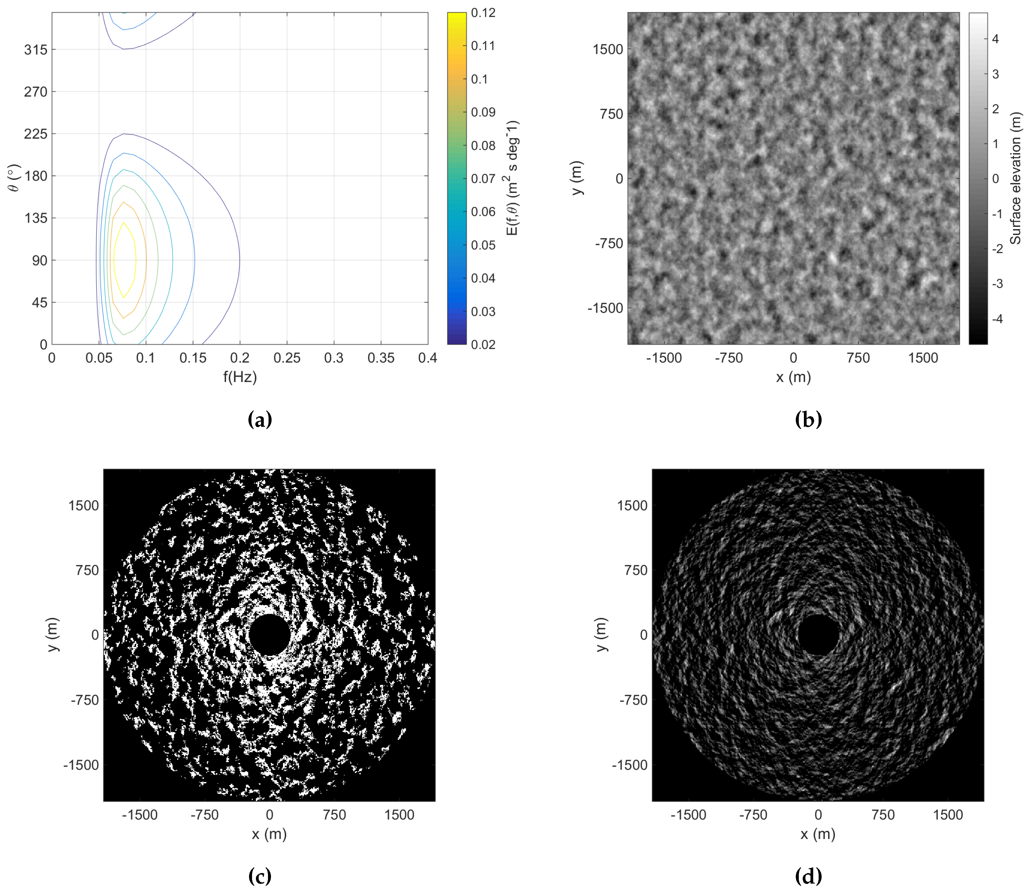
In order to investigate how the shadowing and tilt modulation contribute to the analysis window orientation dependency, the Pierson-Moskowitz-based power distribution model that is recommended by the 15th International Towing Tank Conference (ITTC) [29] and a squared cosine distribution (accounting for angular spreading) [4], with random phases that are generated using a uniform distribution, were used to simulate ocean surface elevation using the directional spectrum in Figure 2a and the parameters listed in Table 1. Figure 2b shows a sample of the simulated surface elevation. The shadowing and tilt masks were calculated for the simulated image sets using the model proposed by Nieto et al. [4]. 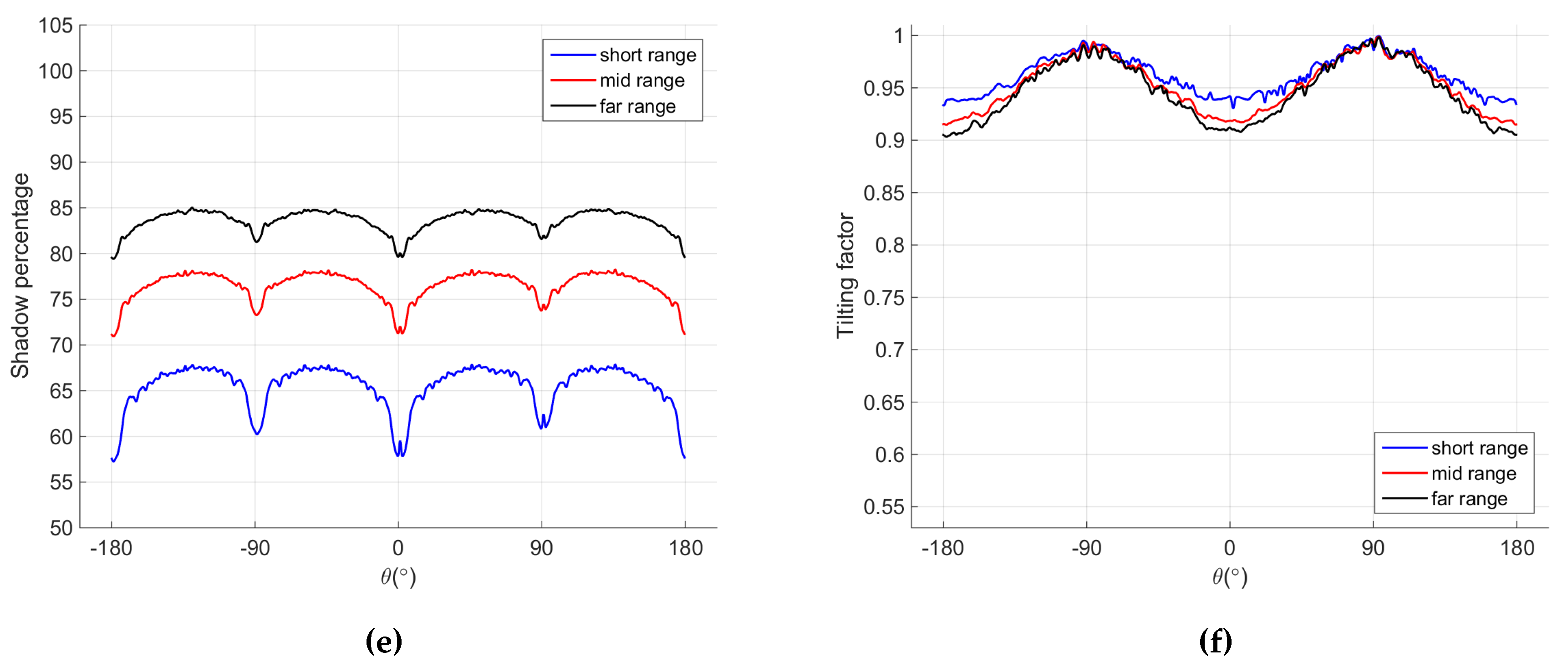Figure 2c,d show the shadowing and tilt masks, respectively. The shadowing percentage is calculated at near, mid and far range as a function of θ. At a certain angle ${\theta }_0$, the shadowing percentage is quantified as the number of shadowed samples within a one dimensional rectangular window applied in the range dimension divided by the window size. Using a window size of 128 samples is more meaningful in this context since the two dimensional analysis window ($128\times 128$ or $256\times 128$) has the same range size. Figure 2e shows the averaged shadowing percentage for 150 simulated radar image sets. Clearly, the shadowing increases with the range. This should not be surprising since the probability that a smaller wave is hidden by a bigger one increases with smaller grazing angles (increasing range). Another interesting observation is that the shadowing is minimum at cross-wave ($\theta =0^{\circ }$ and 180${}^{\circ }$), up-wave ($\theta ={90}^{\circ }$) and down-wave ($\theta =-{90}^{\circ }$) directions. This behavior of the shadowing at these angles is not clear to us and will be investigated in future work. The minimum shadowing at the cross-wave (i.e., parallel to the wave front) direction can be explained by the fact that, at this angle, radar signals travel in parallel with the ocean wave front rather than facing it, giving a smaller opportunity for the shadowing to occur.

Figure 2. Simulation analysis for shadowing and tilting (a–f): (a) Directional wave spectrum used to generate simulated radar images; (b) Simulated surface elevation; (c) Shadowing mask; (d) Tilting mask; (e) Shadowing percentage dependency on the azimuthal direction; (f) Tilting factor dependency on the azimuthal direction.

Figure 2. Simulation analysis for shadowing and tilting (a–f): (a) Directional wave spectrum used to generate simulated radar images; (b) Simulated surface elevation; (c) Shadowing mask; (d) Tilting mask; (e) Shadowing percentage dependency on the azimuthal direction; (f) Tilting factor dependency on the azimuthal direction.

Table 1. Experiment setup: Simulation parameters.

Image set size	$512\times 512\times 32$ samples
Antenna rotational period	1.44 s
Antenna height	10 m
Sampling frequency	20 MHz
Water depth	200 m
Wind wave direction	${90}^{\circ }$ from the true north
Surface current	0.5 m/s ${90}^{\circ }$ from the true north
The mean period $T_{01}$	10 s
The significant wave height	3.5 m

Table 1. Experiment setup: Simulation parameters.

Image set size	$512\times 512\times 32$ samples
Antenna rotational period	1.44 s
Antenna height	10 m
Sampling frequency	20 MHz
Water depth	200 m
Wind wave direction	${90}^{\circ }$ from the true north
Surface current	0.5 m/s ${90}^{\circ }$ from the true north
The mean period $T_{01}$	10 s
The significant wave height	3.5 m

In order to investigate the effect of tilt modulation, it is calculated at near, mid and far ranges as a function of θ in a manner similar to that for the shadowing case. However, tilt modulation is quantified by integrating the shadowing signal over the range within a 128 sample one-dimensional rectangular window. Figure 2f shows the normalized averaged tilting for the simulated image sets. The figure shows peaks at up-wave ($\theta ={90}^{\circ }$) and down-wave ($\theta =-{90}^{\circ }$) directions and minima at cross-wave ($\theta =0^{\circ }$ and 180${}^{\circ }$) for all ranges. This analysis strongly indicates that the azimuthal direction biases the radar imaging mechanisms and by extension the wave spectrum estimation. Also, it can be concluded that for best results in wave spectrum estimation, the analysis window should be chosen in the up-wave direction where the shadowing is minimum since higher shadowing induces higher order dispersion modes [22]. Also, the radar return is strongest in the up-wave direction due to the high tilting factor and Bragg scattering.

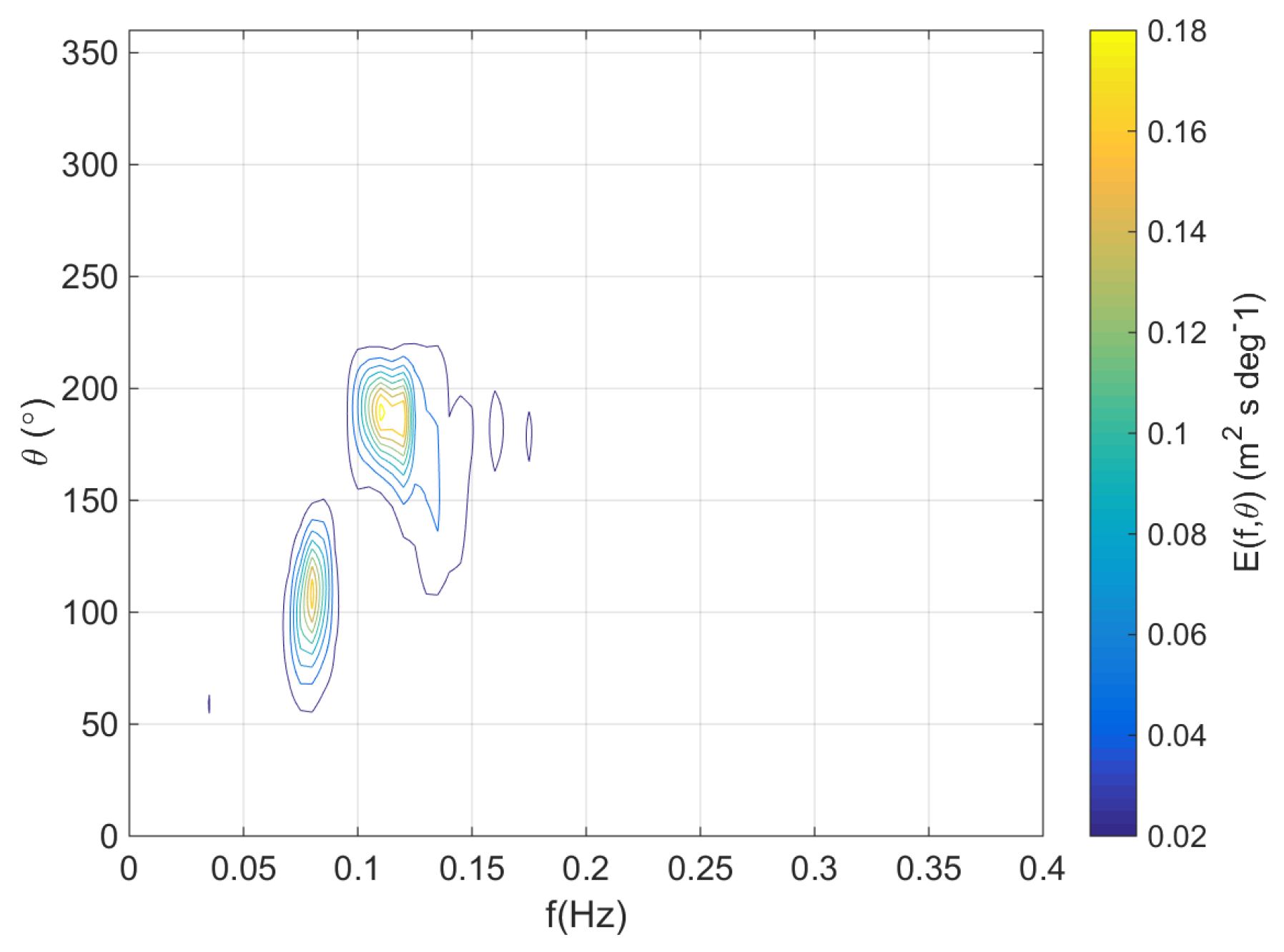
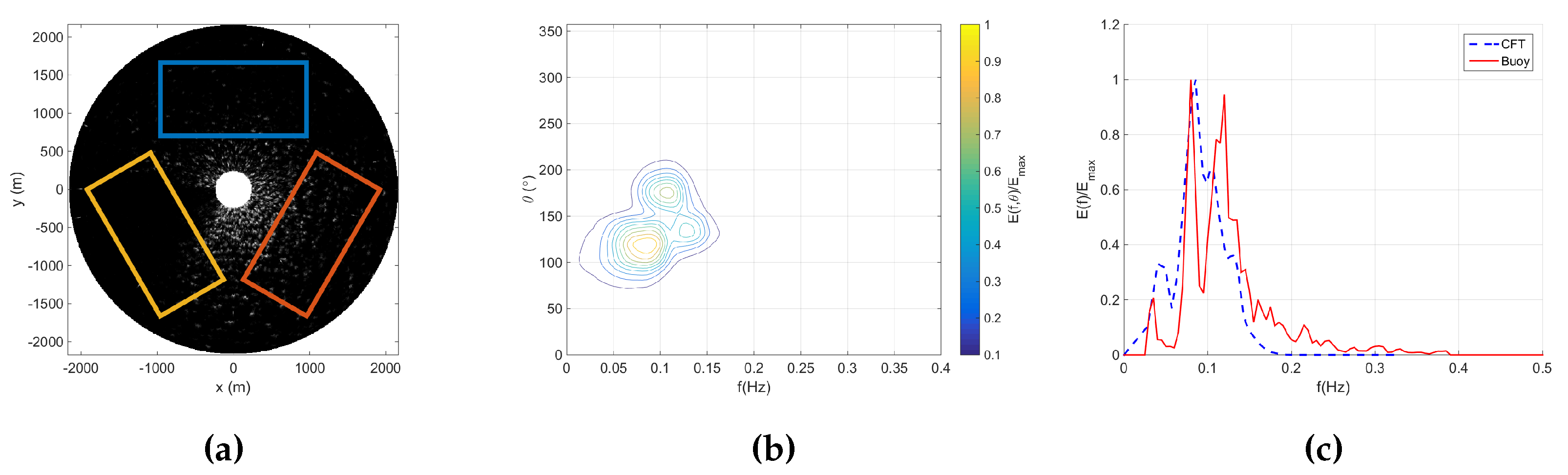
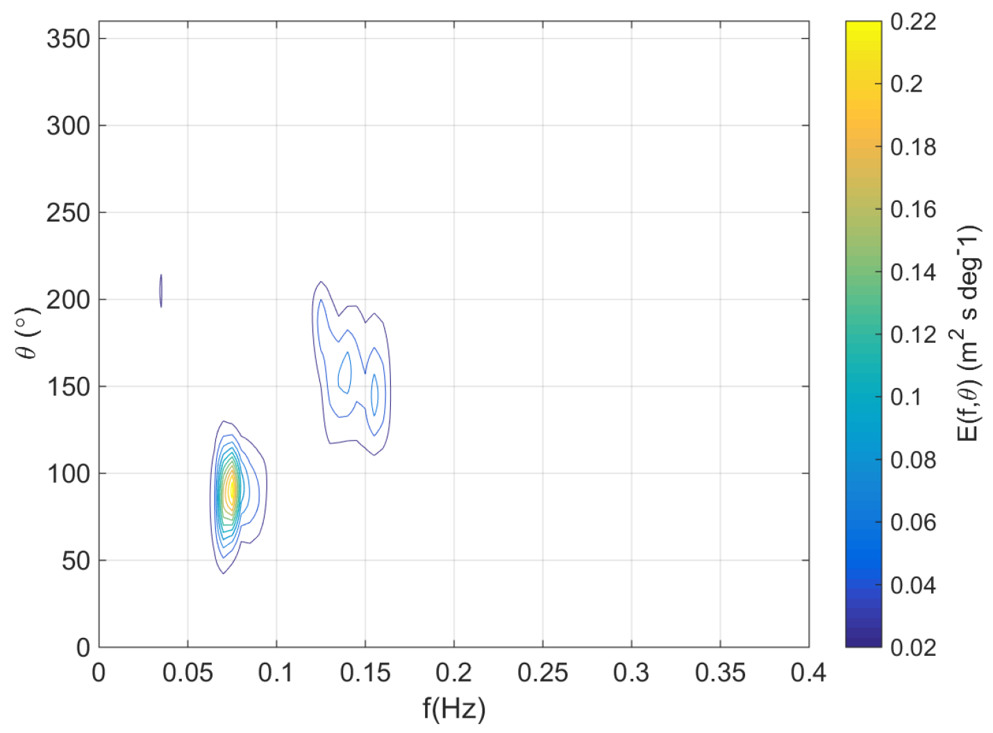
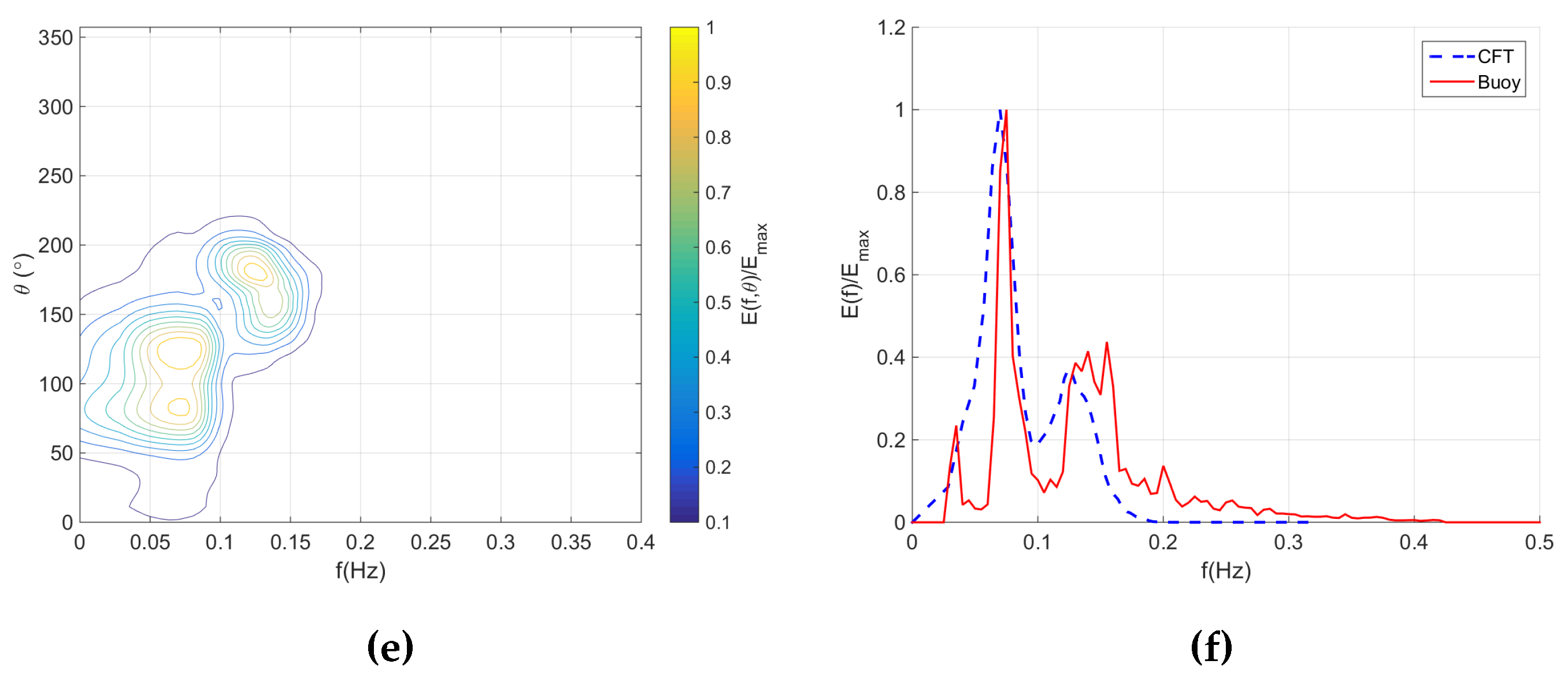
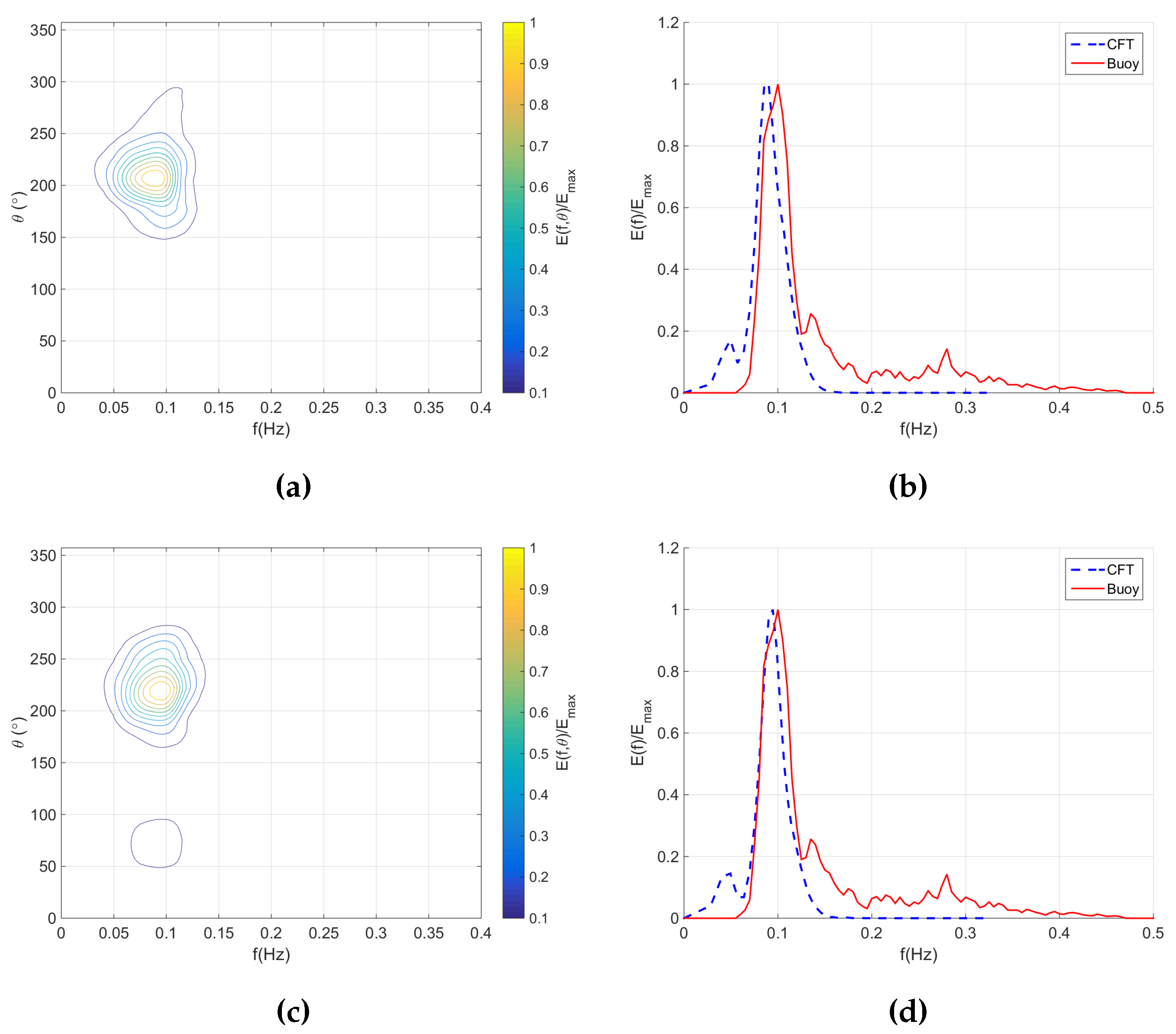
The wave spectrum usually has one or two peaks that are related to wind waves or/and swell. The dominant wind wave and swell do not necessarily travel in the same direction. Therefore, choosing the analysis window in the wind wave direction might occur at the price of compromising the swell peak or vice versa. Traditionally, this problem is addressed by averaging the output of three uniformly distributed analysis windows. 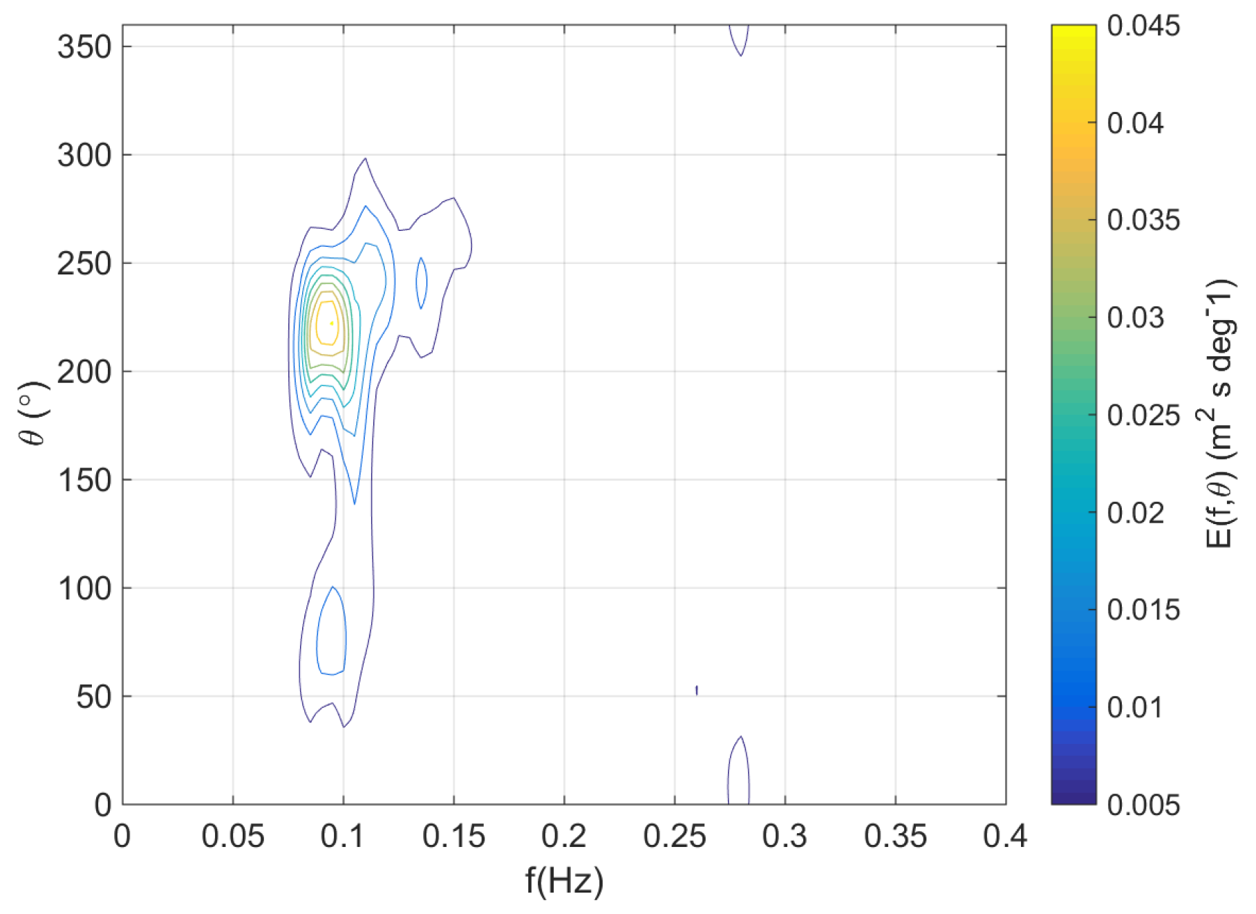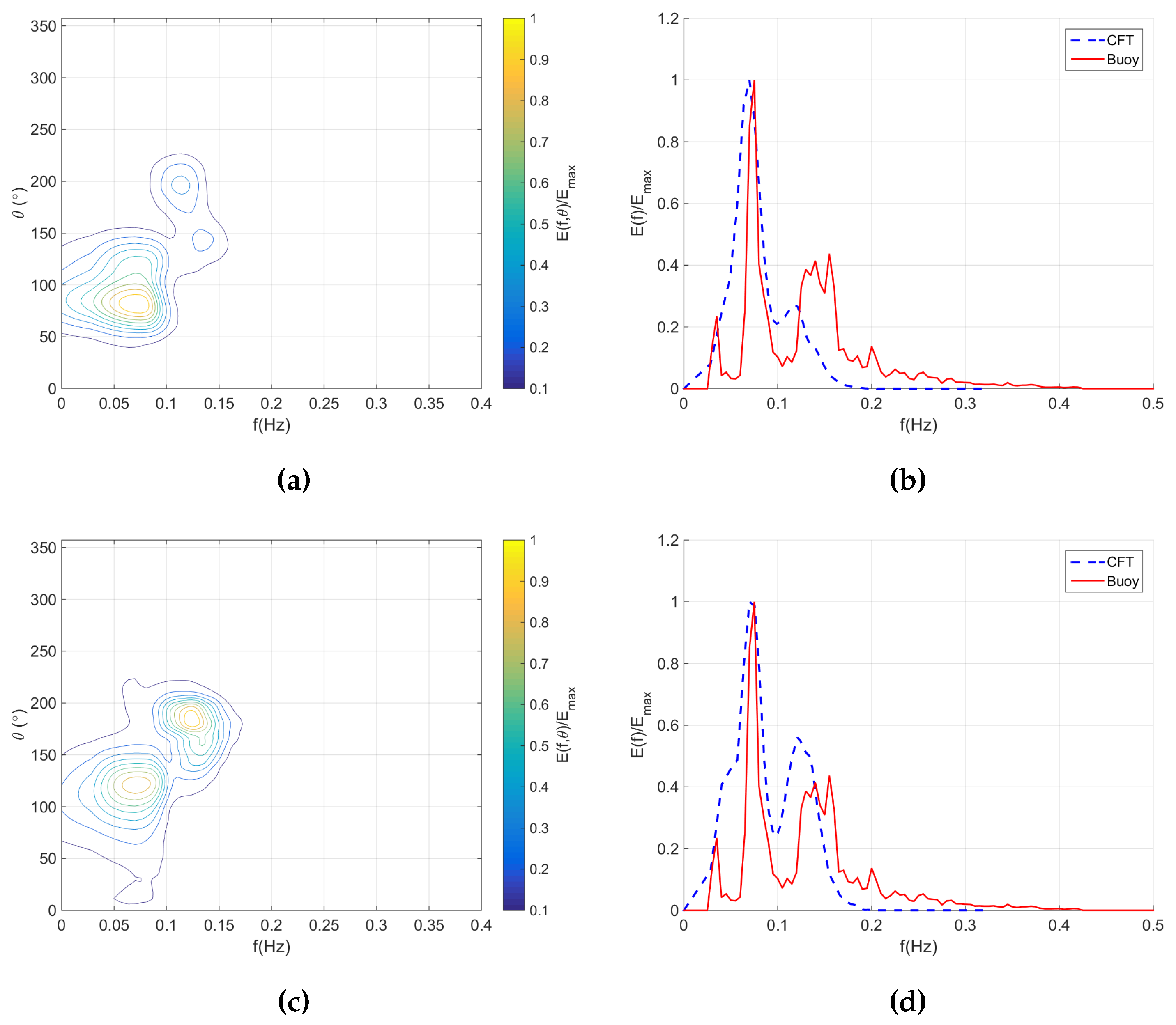For a field data example, Figure 3 shows a directional wave spectrum which is calculated using wave rider buoy data and has two peaks at $\theta ={110}^{\circ }$ and ${185}^{\circ }$.The directional wave spectrum estimated using marine radar data with three analysis windows (see Figure 4a) is presented in Figure 4b. The directional wave spectrum from each window is acquired using the CFT-based method outlined in Section 2 and detailed in [4,6,30]. In this example, the buoy is located in the radar range. Clearly, both peaks in the directional wave spectrum of the buoy are detected in the radar’s wave spectrum. 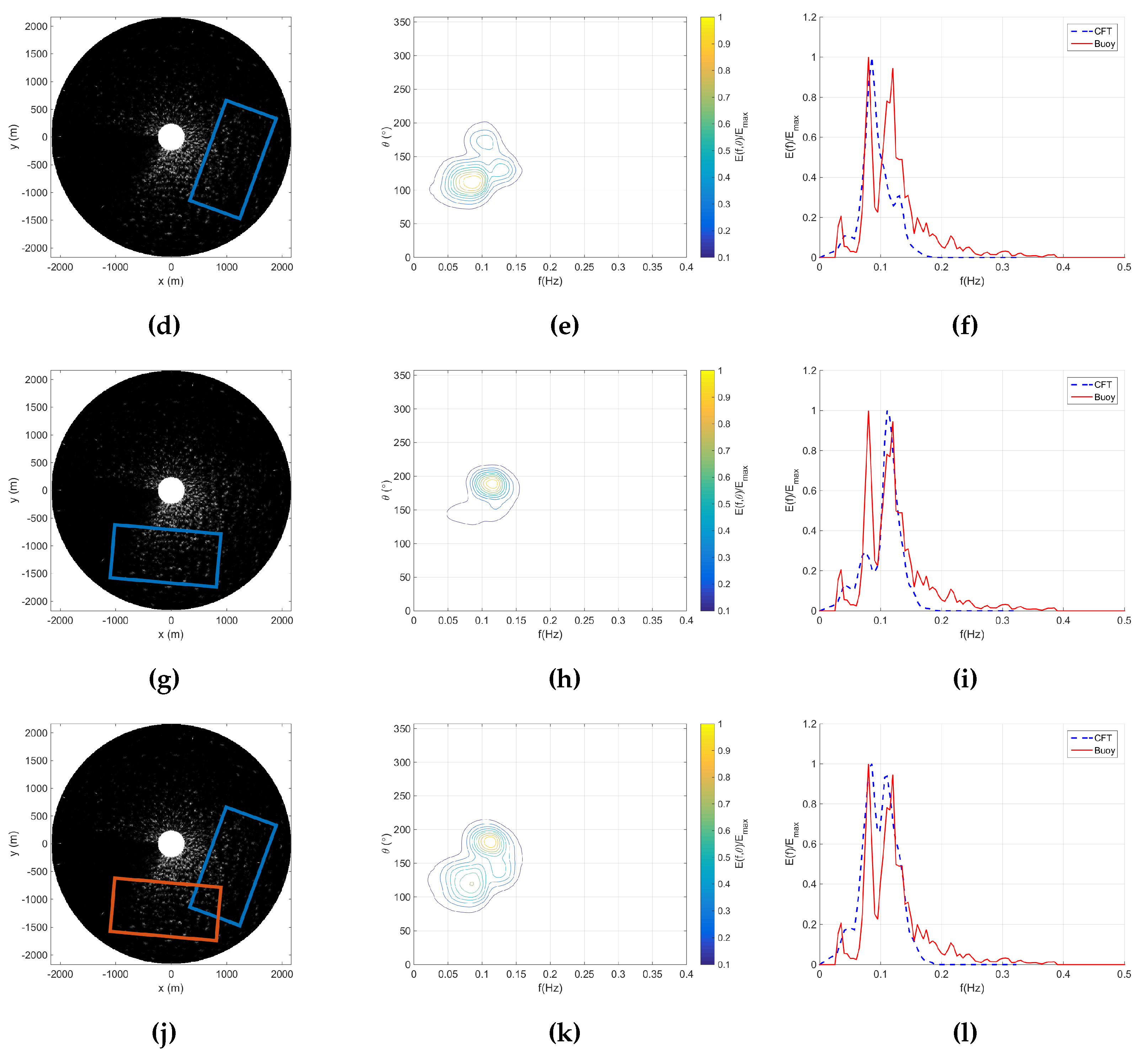However, comparing the normalized non-directional wave spectrum in Figure 4c, which is calculated using Equation (5) and divided by its maximum value, it may be seen that the second peak is almost non-distinguishable. 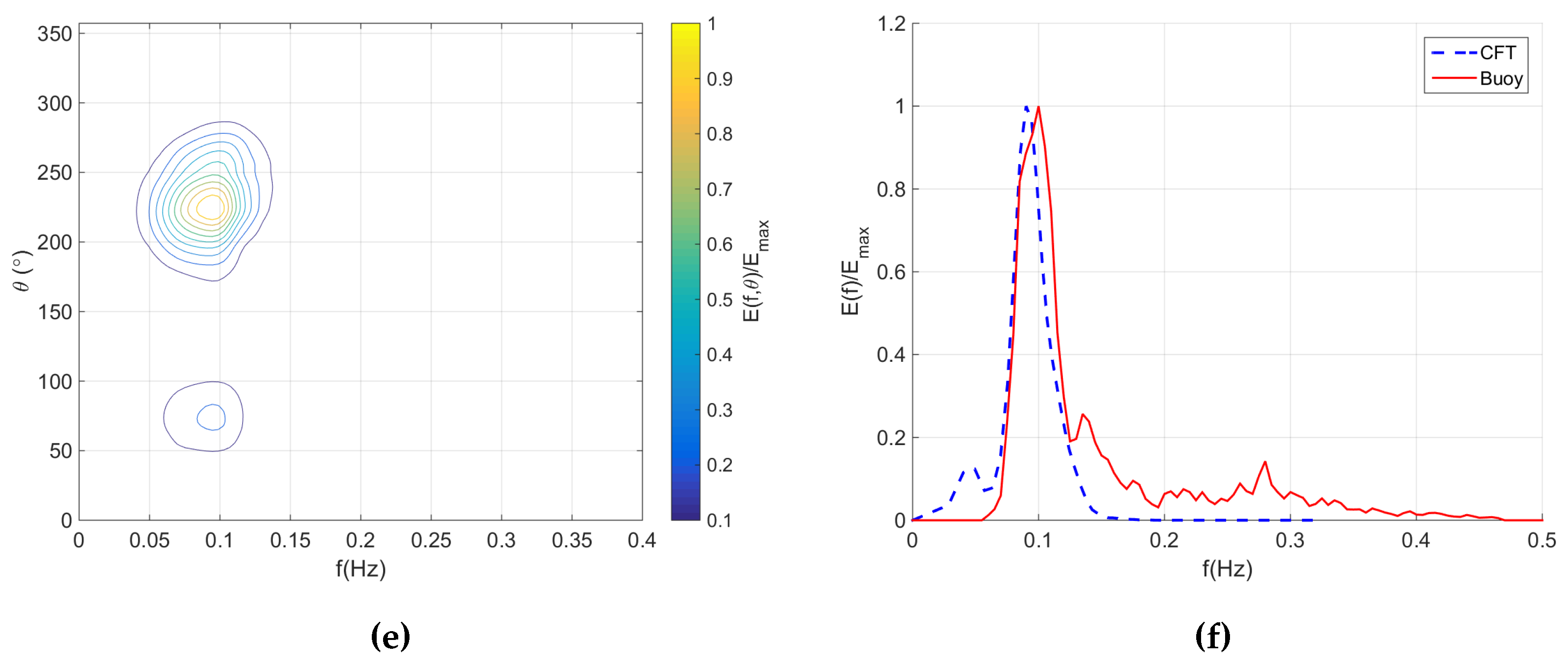Now, when taking the analysis window orientation to be in the first peak direction, $\theta ={110}^{\circ }$ (see Figure 4d), the first peak is even more emphasized compared to the second one which is completely non-distinguishable as shown in Figure 4e,f. When taking the analysis window in the direction of the second peak ($\theta ={185}^{\circ }$), Figure 4g–i show more weight for the second peak over the first which now has an energy level of 25% compared to 100% of the first peak for the ground truth. Finally, an intuitive solution is to average the results from the two analysis windows which are in the direction of spectral peaks at $\theta ={110}^{\circ }$ and ${185}^{\circ }$ (see Figure 4j). Figure 4k,l show better agreement with the buoy estimated spectrum. However, this approach is challenging since the wave directions are not known beforehand. In this paper, we propose a new method referred to as the Adaptive Recursive Positioning Method (ARPM); this method estimates the direction of travel of the waves and chooses the analysis windows orientation accordingly.

Figure 3. Directional wave spectrum for example given in Figure 4. Directional wave spectrum is estimated using a directional TRIAXYS wave rider buoy.

Figure 3. Directional wave spectrum for example given in Figure 4. Directional wave spectrum is estimated using a directional TRIAXYS wave rider buoy.

Figure 4. A field data example for wave spectrum estimation dependency on azimuth direction(a–l). Data was recorded on 1 December 2008 at 4:38 PM :(a,d,g,j) A single Furuno radar image shows various analysis window orientations; (b,e,h,k) The directional wave spectrum estimated using the CFT on the analysis windows in figures (b), (e), (h) and (k), respectively; (c,f,i,l) The frequency wave spectrum estimated using the CFT on the analysis windows in figures (a), (d), (g) and (j), respectively overlaid on the ground truth frequency wave spectrum.

Figure 4. A field data example for wave spectrum estimation dependency on azimuth direction(a–l). Data was recorded on 1 December 2008 at 4:38 PM :(a,d,g,j) A single Furuno radar image shows various analysis window orientations; (b,e,h,k) The directional wave spectrum estimated using the CFT on the analysis windows in figures (b), (e), (h) and (k), respectively; (c,f,i,l) The frequency wave spectrum estimated using the CFT on the analysis windows in figures (a), (d), (g) and (j), respectively overlaid on the ground truth frequency wave spectrum.

4. The Adaptive Recursive Positioning Method (ARPM)

The ARPM determines the number and orientation of the analysis windows according to the number and orientation of peaks in the wave spectrum. In the case where the wave spectrum has only one peak, one analysis window is chosen in the direction of that peak. In the case where the wave spectrum consists of two peaks resulting from wind waves and swell, two analysis windows are chosen in the directions of these peaks. For instances where the wave spectrum may consist of $n>2$ peaks, n analysis windows are used and positioned in the peak directions. Since the wave spectrum is not known beforehand, the ARPM determines the analysis window locations recursively. 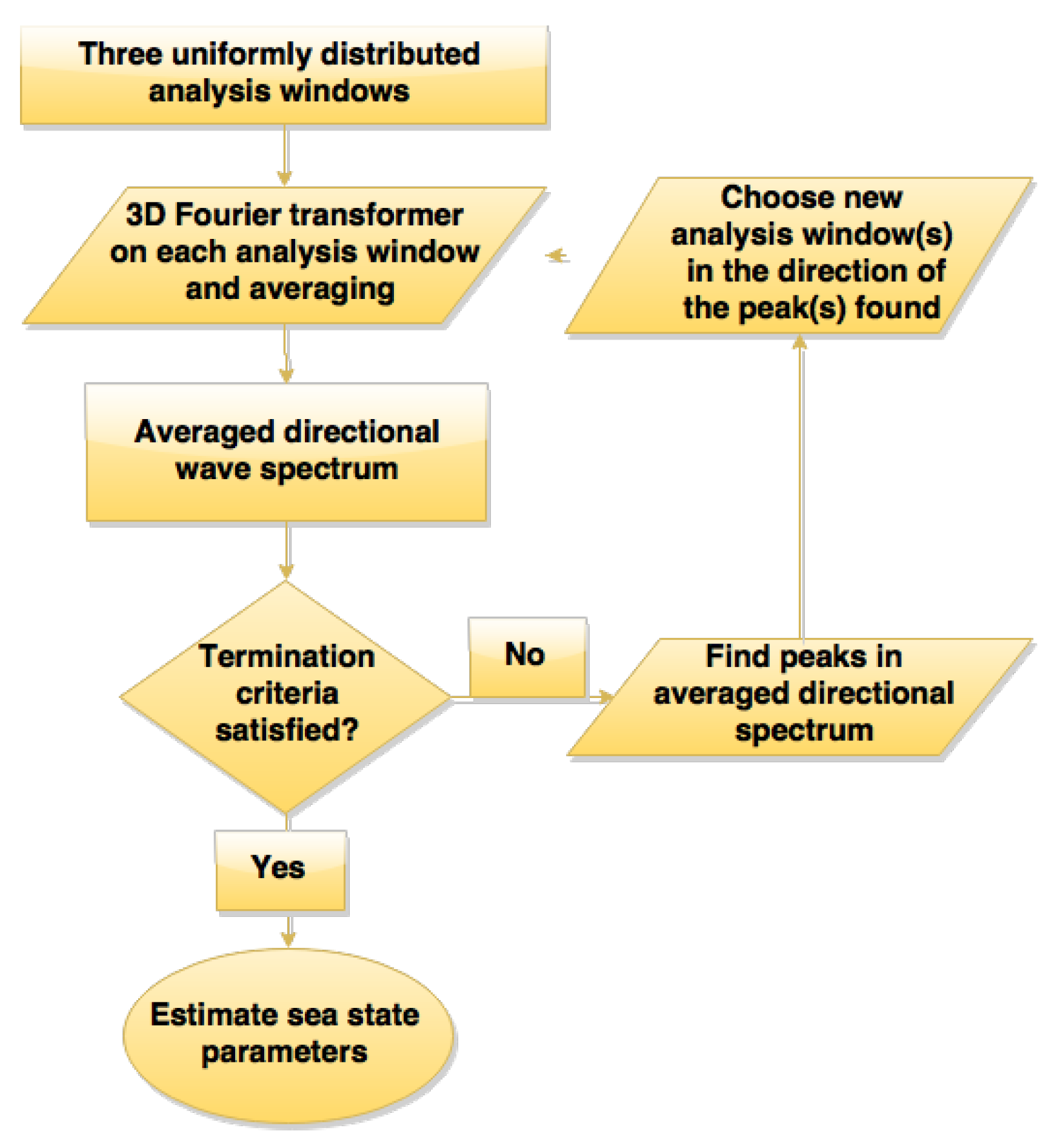Figure 5 shows the flowchart of the ARPM. 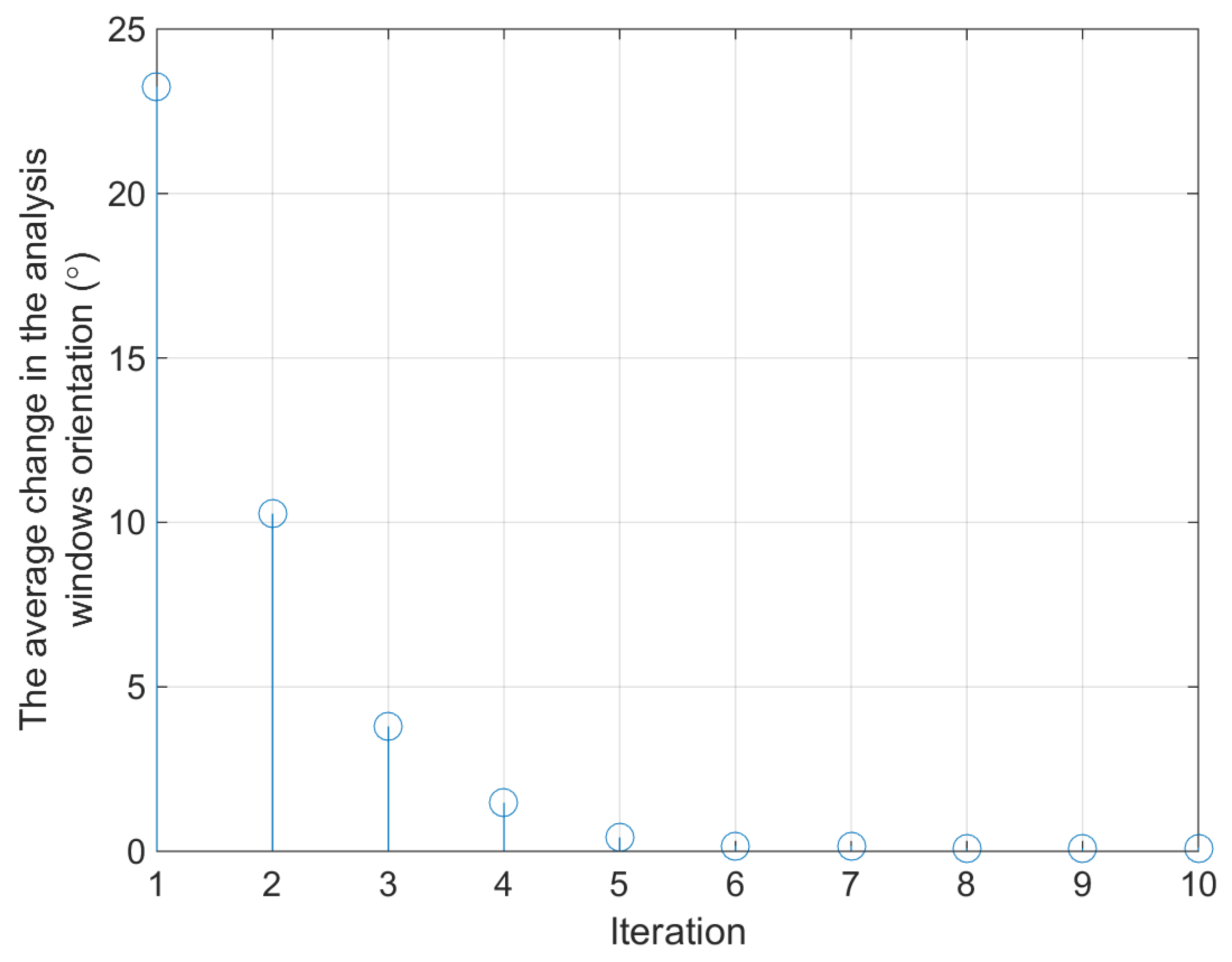The method starts by estimating the wave spectrum using three uniformly distributed analysis windows in a manner that is similar to the standard method outlined in Section 3. The estimated directional wave spectrum is used as an initial estimate to determine the number and direction of the peaks. Subsequently new analysis window(s) are chosen in the direction(s) of the peaks, and a new estimation of the wave spectrum is obtained. This process is repeated until a termination criterion is satisfied. For the results of this paper, a simple termination criterion is used which limits the number of iterations to a maximum number. Three iterations were found to generate satisfactory results after which little change in the number and orientation of the analysis windows was noticed. While Figure 6 shows a continuous decrease in the average change in the orientation of the analysis windows to iteration 5 or 6, however, trading off analysis cost and estimate accuracy, 3 iterations were found to be sufficient.

Figure 5. Adaptive Recursive Positioning Method (ARPM) flowchart.

Figure 5. Adaptive Recursive Positioning Method (ARPM) flowchart.

Figure 6. The average change in the analysis windows’ orientation for different numbers of iterations in the ARPM.

Figure 6. The average change in the analysis windows’ orientation for different numbers of iterations in the ARPM.

Obviously this method needs a full field of view or in practice close to it. This is needed to facilitate the freedom in choosing the orientation of the analysis window(s). Usually data from offshore platforms and shipboard marine radars provide such a field of view. On the other hand, coastal station marine radars might not provide such a wide ocean field of view.

5. Experiment Setup and Data Overview

In order to examine the efficiency of the proposed algorithm, the ARPM has been applied to field data collected near Halifax, Nova Scotia, on East Coast of Canada (see Figure 7 and Table 2) by shipborne Decca and Furuno X-band nautical radars over a 10 day period. The radars that were connected to a Wave Monitoring System II (WaMoS II) were operating at 9.4 GHz with HH polarization and at grazing incidence. The results from the ARPM were validated by comparison with ground truth data provided from a TRIAXYS wave rider buoy. During the experiment, there was a drift of 41 km in the wave buoy location. However, the radars were always within a 10 km distance of the buoy, which generated a reading every 30 min. The directional spectrum from the wave buoy covers a frequency range of 0.030 to 0.465 Hz with a 0.005 Hz resolution over a full 360${}^{\circ }$ azimuth with 3${}^{\circ }$ resolution. Since the radar’s antenna rotational time was 1.44 s, our frequency spectrum analysis and comparison are limited to the range of 0.05 to 0.35 Hz. Table 2 lists further radar details. The modulation transfer function $MTF={\left|\mathbf{k}\right|}^{-1.2}$ is used in our analysis [4]. A single estimate using our method required a 32-image set and an analysis window of size 256 × 128 samples. For better results and compatibility with the wave buoy output, the wave spectrum estimated from the ARPM was averaged over the same period (30 min) of time.

Figure 7. Locations of wave buoy and radar during the experiment on 1 December 2008.

Figure 7. Locations of wave buoy and radar during the experiment on 1 December 2008.

Table 2. Experiment setup: Radar and buoy parameters.

Experiment location	42${}^{\circ }$22.4391N 61${}^{\circ }$55.5654W
Antenna rotational time	1.44 s
Antenna height	10 m
Sampling frequency	20 MHz
Water depth	200 m
Polarization	Horizontal
TRIAXYS wave period accuracy	better than 1%
TRIAXYS wave direction accuracy	$1^{\circ }$

Table 2. Experiment setup: Radar and buoy parameters.

Experiment location	42${}^{\circ }$22.4391N 61${}^{\circ }$55.5654W
Antenna rotational time	1.44 s
Antenna height	10 m
Sampling frequency	20 MHz
Water depth	200 m
Polarization	Horizontal
TRIAXYS wave period accuracy	better than 1%
TRIAXYS wave direction accuracy	$1^{\circ }$

6. Results and Analysis

6.1. Field Data Examples

In order to demonstrate the accuracy of the ARPM, we start by an example. Figure 8 shows a ground truth wave spectrum which is estimated from TRIAXYS wave buoy data. The spectrum has a main peak at 0.075 Hz and 90${}^{\circ }$ and a secondary peak at 0.15 Hz and 150${}^{\circ }$. Figure 9 shows the ARPM output for each iteration. The estimated directional and frequency wave spectrum in the first iteration (standard method) is shown in Figure 9a,b, respectively. The secondary peak was underestimated with a lower relative energy level of 25%, relative to that of the main peak of the first iteration, compared to 40% for the ground truth secondary peak. In the second iteration, only two analysis windows are used, and they are repositioned to be in the peak directions. The estimated directional and frequency wave spectra of the second iteration are shown in Figure 9c,d, respectively. Clearly, the secondary peak is better estimated in this iteration with a higher relative energy level of 60%, relative to that of the main peak of the second iteration, compared to its estimate in the first iteration of 25%. However, further refinement is needed since it now has more relative energy than the ground truth and thus can be deemed to be over-estimated. Finally, the last iteration produces a satisfactory improvement in the estimated wave spectra as shown in Figure 9e,f. The secondary peak is now almost at the same relative energy level (40%) as in the ground truth spectrum.

Figure 8. Directional wave spectrum for example given in Figure 9. Directional wave spectrum is estimated using a directional TRIAXYS wave rider buoy.

Figure 8. Directional wave spectrum for example given in Figure 9. Directional wave spectrum is estimated using a directional TRIAXYS wave rider buoy.

Figure 9. A field data example for wave spectrum estimation using the CFT with the ARPM. Data was recorded on 1 December 2008 at 12:08 PM (a–f): (a,c,e) The directional wave spectrum estimated in the first, second and third iteration, respectively; (b,d,f) The frequency wave spectrum estimated from the radar data in the first, second and third iteration respectively and overlaid on the ground truth frequency wave spectrum.

Figure 9. A field data example for wave spectrum estimation using the CFT with the ARPM. Data was recorded on 1 December 2008 at 12:08 PM (a–f): (a,c,e) The directional wave spectrum estimated in the first, second and third iteration, respectively; (b,d,f) The frequency wave spectrum estimated from the radar data in the first, second and third iteration respectively and overlaid on the ground truth frequency wave spectrum.

Another example is shown in Figure 10. Figure 11 shows a ground truth wave spectrum which is estimated using a TRIAXYS wave buoy data. The spectrum has two peaks, a main peak at 0.09 Hz and 225${}^{\circ }$ and a secondary peak at 0.09 Hz and 75${}^{\circ }$. Obviously, these peaks are not distinguished through the frequency spectrum because both peaks are at 0.09 Hz. Looking at the directional wave spectrum in Figure 10a produced in the first iteration, the secondary peak is not detected. Comparing this estimate to the final estimate produced in the final iteration (Figure 10e), the secondary peak is now visible.

Figure 10. A field data example for wave spectrum estimation using the CFT with the ARPM. Data was recorded on 3 December 2008 at 5:31 AM (a–f): (a,c,e) The directional wave spectrum estimated in the first, second and third iteration, respectively; (b,d,f) The frequency wave spectrum estimated from the radar data in the first, second and third iteration respectively and overlaid on the ground truth frequency wave spectrum.

Figure 10. A field data example for wave spectrum estimation using the CFT with the ARPM. Data was recorded on 3 December 2008 at 5:31 AM (a–f): (a,c,e) The directional wave spectrum estimated in the first, second and third iteration, respectively; (b,d,f) The frequency wave spectrum estimated from the radar data in the first, second and third iteration respectively and overlaid on the ground truth frequency wave spectrum.

Figure 11. Directional wave spectrum for example given in Figure 10. Directional wave spectrum is estimated using a directional TRIAXYS wave rider buoy.

Figure 11. Directional wave spectrum for example given in Figure 10. Directional wave spectrum is estimated using a directional TRIAXYS wave rider buoy.

6.2. Performance Validation

The last two examples show that the ARPM significantly improves the wave spectrum estimation over the standard method. In order to validate the performance of the ARPM, the agreement between its estimated wave spectrum and the buoy wave spectrum (the ground truth) is quantified using the correlation coefficient between the two frequency spectra on a discrete frequency grid. The value of the correlation coefficient ranges from 0 (no similarity) to 1 (identical). As mentioned before, one radar set (32 images) is used to calculate a wave spectrum estimate. The estimates from 30 sets are averaged to be compared with one buoy spectrum estimate. The standard method and the ARPM are used to estimate the wave spectrum. The correlation coefficient with the buoy ground truth is calculated for each method. Figure 12 shows the correlation coefficient in pairs: the standard method coefficient is marked using a “o” while the ARPM is marked using a “ × ”; the results are shown for four days during the experiment (27 November, 29 November, 2 December and 3 December of 2008). To enhance the readability of the results, the ARPM output is plotted in blue (red) to indicate improvement (deterioration) in performance compared to the standard method. Clearly, the ARPM outperforms the standard method with higher correlation coefficients except for a few cases. The averaged improvement is found to be 9.8%.

Figure 12. A comparison between the ARPM and the standard method in terms of the frequency wave spectrum similarity with respect to the buoy ground truth spectra. Each point represents the correlation coefficient between ground truth and the radar data 30 min averaged frequency wave spectra. (a–d) 27 November, 29 November, Dec 1 and 3 December respectively.

Figure 12. A comparison between the ARPM and the standard method in terms of the frequency wave spectrum similarity with respect to the buoy ground truth spectra. Each point represents the correlation coefficient between ground truth and the radar data 30 min averaged frequency wave spectra. (a–d) 27 November, 29 November, Dec 1 and 3 December respectively.

For further validation, the peak wave period $T_p$, mean period $T_{01}$, the zero-crossing period $T_z$ and the peak wave direction ${\theta }_p$ are estimated for wind waves and swell using the standard method and the ARPM. Figure 13 and Figure 14 show the peak wave period and direction, respectively. The mean absolute error ($\overline{\left|{\epsilon }_{T_p}\right|}$,$\overline{\left|{\epsilon }_{T_{01}}\right|}$, $\overline{\left|{\epsilon }_{T_z}\right|}$ and $\overline{\left|{\epsilon }_{{\theta }_p}\right|}$) and error standard deviation (${\sigma }_{{\epsilon }_{T_p}}$, ${\sigma }_{{\epsilon }_{T_{01}}},$ ${\sigma }_{{\epsilon }_{T_z}}$ and ${\sigma }_{{\epsilon }_{{\theta }_p}}$) of these estimates are calculated with respect to the ground truth and listed in Table 3. The mean absolute error and the error standard deviation of $T_p$ are given by

$$\overline{\left|{\epsilon }_{T_p}\right|}=\frac{1}{N}\sum _{n=1}^N|T_{p_n}-T_{pBuo{y}_n}|$$

(7)

and

$${\sigma }_{{\epsilon }_{T_p}}=\sqrt{\frac{1}{N}\sum _{n=1}^N{\left(T_{p_n}-\frac{1}{N}\sum _{m=1}^N,T_{p_m}\right)}^2}$$

(8)

respectively, where N is the total number of radar estimates and $T_{pBuoy}$ is the ground truth of $T_p$. The other metrics are calculated in a similar manner.

Figure 13. A comparison between the ARPM and the standard method in terms of the peak wave period. (a–d) 27 November, 29 November, 1 December and 3 December respectively.

Figure 13. A comparison between the ARPM and the standard method in terms of the peak wave period. (a–d) 27 November, 29 November, 1 December and 3 December respectively.

Figure 14. A comparison between the ARPM and the standard method in terms of the peak wave direction. (a–d) 27 November, 29 November, 1 December and 3 December respectively.

Figure 14. A comparison between the ARPM and the standard method in terms of the peak wave direction. (a–d) 27 November, 29 November, 1 December and 3 December respectively.

Finally, it is not surprising that this improvement comes at the price of extra computational time. As an illustration, in our analysis and implementation, the standard method needed 2.7 s to process one radar set (32 radar images) while the ARPM required 5 s, with both implementations running on the same processor and with similar software and data structure efficiency. However, this price is very reasonable since the time needed by the radar to generate one data set is 48 s. Therefore, the ARPM can be also used for real-time analysis.

Table 3. Comparison of the ARPM and the standard method in wave period and peak direction estimation.

	$\overline{|{\epsilon }_{T_p}|}$(s)	${\sigma }_{{\epsilon }_{T_p}}$ (s)	$\overline{|{\epsilon }_{T_{01}}|}$(s)	${\sigma }_{{\epsilon }_{T_{01}}}$ (s)	$\overline{|{\epsilon }_{T_z}|}$(s)	${\sigma }_{{\epsilon }_{T_z}}$(s)	$\overline{|{\epsilon }_{{\theta }_p}|}$(${}^{\circ }$)	${\sigma }_{{\epsilon }_{{\theta }_p}}$(${}^{\circ }$)
standard	3.7	5.1	3.5	4.7	3.5	4.7	14	17
ARPM	2.0	3.1	1.9	3.0	1.9	3.0	8	10

Table 3. Comparison of the ARPM and the standard method in wave period and peak direction estimation.

	$\overline{|{\epsilon }_{T_p}|}$(s)	${\sigma }_{{\epsilon }_{T_p}}$ (s)	$\overline{|{\epsilon }_{T_{01}}|}$(s)	${\sigma }_{{\epsilon }_{T_{01}}}$ (s)	$\overline{|{\epsilon }_{T_z}|}$(s)	${\sigma }_{{\epsilon }_{T_z}}$(s)	$\overline{|{\epsilon }_{{\theta }_p}|}$(${}^{\circ }$)	${\sigma }_{{\epsilon }_{{\theta }_p}}$(${}^{\circ }$)
standard	3.7	5.1	3.5	4.7	3.5	4.7	14	17
ARPM	2.0	3.1	1.9	3.0	1.9	3.0	8	10

7. Conclusions and Future work

The best orientation of the analysis window should be in the up-wave direction where the effects of shadowing and tilt modulation are minimum and the backscatter intensity is maximum due to stronger Bragg scattering. However, in the presence of wind waves and swell, the situation is more challenging since choosing the orientation of the analysis window in the direction of one of the sets of waves (wind waves or swell) is at the price of underestimating the other one. For this reason, in this paper, we propose to use multiple analysis windows oriented in the directions of wind waves and swell. This approach presents another challenge which is that the wind wave and/or the swell directions are not known a priori. Therefore, this paper proposes the Adaptive Recursive Position Method (ARPM) to solve this problem by finding the number and orientation of analysis windows recursively. The ARPM presented significant improvement in wave spectrum estimation that has been demonstrated by producing frequency spectra that better agree with ground truth data. It has also been shown that the ARPM can enable more accurate and reliable wave period and direction estimates compared to the standard method. Currently, we are testing and validating the performance of the ARPM in surface current estimation. Our preliminary analysis and results indicate that the ARPM may significantly improve surface current estimation as well.

Future work on the ARPM concerns expanding its functionality for cases where field of view is partially blocked. This can be addressed by using the available field of view to determine an initial estimate. If the up-wave direction lies in the available part of the field of view, the ARPM can proceed normally. Otherwise, the algorithm would terminate and the initial estimate would be used.