Article

Distinguishing Early Successional Plant Communities Using Ground-Level Hyperspectral Data

Department of Environmental Sciences, University of Virginia, 291 McCormick Road, Charlottesville, VA 22903, USA
*
Author to whom correspondence should be addressed.
Remote Sens. 2015, 7(12), 16588-16606; https://doi.org/10.3390/rs71215850
Submission received: 25 September 2015 / Revised: 24 November 2015 / Accepted: 27 November 2015 / Published: 8 December 2015
(This article belongs to the Special Issue Remote Sensing of Vegetation Structure and Dynamics)

Abstract

:
Abandoned agricultural fields have recently become more abundant in the U.S. and remain susceptible to species invasions after cultivation disturbance. As invasive species become more widespread with increases in anthropogenic activities, we need more effective ways to use limited resources for conservation of native ecosystems. Remote sensing can help us monitor the spread and effects of invasive species, and thus determine the species and locations to target for conservation. To examine this potential, we studied plant communities dominated by exotic invasive plant species in secondary successional fields in northern Virginia using ground-level hyperspectral data. Within these communities, ordination analyses of vegetation surveys revealed differences in species compositions among plots and fields. These differences among communities were also observed in the spectral data. Stepwise multiple linear regression analyses to determine which species influenced the ordination axes revealed that many of the influential species are considered invasive, again underscoring the influence of invasive species on community properties. Stepwise regression analyses also revealed that the most influential wavelengths for discrimination were distributed along the spectral profile from the visible to the near-infrared regions. A discriminant analysis using wavelengths selected with a principal components analysis demonstrated that different plant communities were separable using spectral data. These spectrally observable differences suggest that we can use hyperspectral data to distinguish among invasive-dominated successional plant communities in this region.

Graphical Abstract

1. Introduction

Abandoned agricultural fields are becoming more prevalent in the U.S., especially in the northeast and midwest [1], and are easily occupied by exotic invasive plant species [2]. These invasive species can alter community composition and ecosystem properties, such as resource availability and use, disturbance frequency, plant community interactions, and the community compositions of herbivores, soil microbes, and birds [3,4,5,6]. These species can also alter community and ecosystem dynamics during secondary succession [4,7]. The invasive species may take advantage of open niches during early succession [8], thus affecting the degree, duration, and direction of ecosystem change. They can have no effect [9], or their effects can be limited to earlier stages of succession with eventual reclamation by natives [10,11]. Alternatively, they can completely change the trajectory, rate, species composition, species richness, disturbance regimes, and nutrient cycling during succession [6,7,12,13,14]. In order to monitor invasive species, we need to develop better methodologies for mapping them at fine space-time resolutions.
The control of these invasive species is resource intensive and, due to the limited availability of such resources as time and funding, conservation strategies must be targeted. To do this, we must determine which species are most detrimental to the environment and can most easily be controlled. Ground-based methods for monitoring invasive species are costly and thus can limit research and management; alternatively, remote sensing can supplement field data to monitor spatial and temporal distributions of invasive species [15,16,17,18].
Multispectral data have been used to observe vegetation characteristics and discriminate among species; as an example, Smith and Blackshaw [19] were able to discriminate among two crop species and five weed species with 89% accuracy using multispectral data with some misclassification of grasses as broad-leaf plants and vice versa. However, hyperspectral data may provide better estimates of such vegetation characteristics and more accurately discriminate species due to more numerous and narrower wavebands [19,20]. In addition to their multispectral analysis, Smith and Blackshaw [19] observed 90% accuracy in discriminating the crop and weed species using hyperspectral data; however, the misclassifications were now within grasses and broad-leaf plants rather than across. Hyperspectral data have recently been used more frequently to distinguish among individual plant species [17,21,22,23,24,25], and we may be able to examine community properties and processes spectrally where certain individual species dominate.
When examining plant species and communities with remote sensing, we need to consider several sources of variation in spectral data. Variation of visible (VIS) reflectance is mostly due to leaf pigment and nutrient content, while variation in the near-infrared (NIR) region is due to leaf structure and surface characteristics; variation in the shortwave infrared (SWIR) region is due to plant water content [26,27]. At the leaf level, reflectance is further influenced by biochemical processes, stress, and phenological processes (e.g., senescence) [27,28]. Spectral signatures also differ between sun and shade leaves, as sun leaves have lower reflectance values along the entire spectral profile than do shade leaves due to greater leaf thickness and pigment concentrations [29]. At the canopy level, vegetation spectra are influenced by foliar reflectance, foliar transmittance, and crown architecture [30]. Certain biological traits that influence spectra also vary in response to changes in the environment; for example, chlorophyll a:chlorophyll b ratios change with illumination [31]. Additionally, absorption bands can be affected by more than one chemical constituent of a leaf, and one chemical constituent can influence a broad spectral region [32].
Such spectral variability in these characteristics may weaken direct correlations between biological properties or processes and spectral data. However, these data can be used to discriminate species and communities if interspecific differences in such characteristics are greater than intraspecific and intra-individual differences [16]. Spectral differences due to diversity in pigment content, water content, structural elements, cell size, intercellular space, and cell wall thickness can assist in differentiating among plant species and communities [33]. In this paper, we ask: (1) Can plant communities in successional fields in a ridge-and-valley system in northern Virginia be distinguished using ground-level hyperspectral remote sensing? (2) Which species are most influential in affecting discriminability? (3) Which spectral variables explain the greatest variance in community composition?

2. Experimental Section
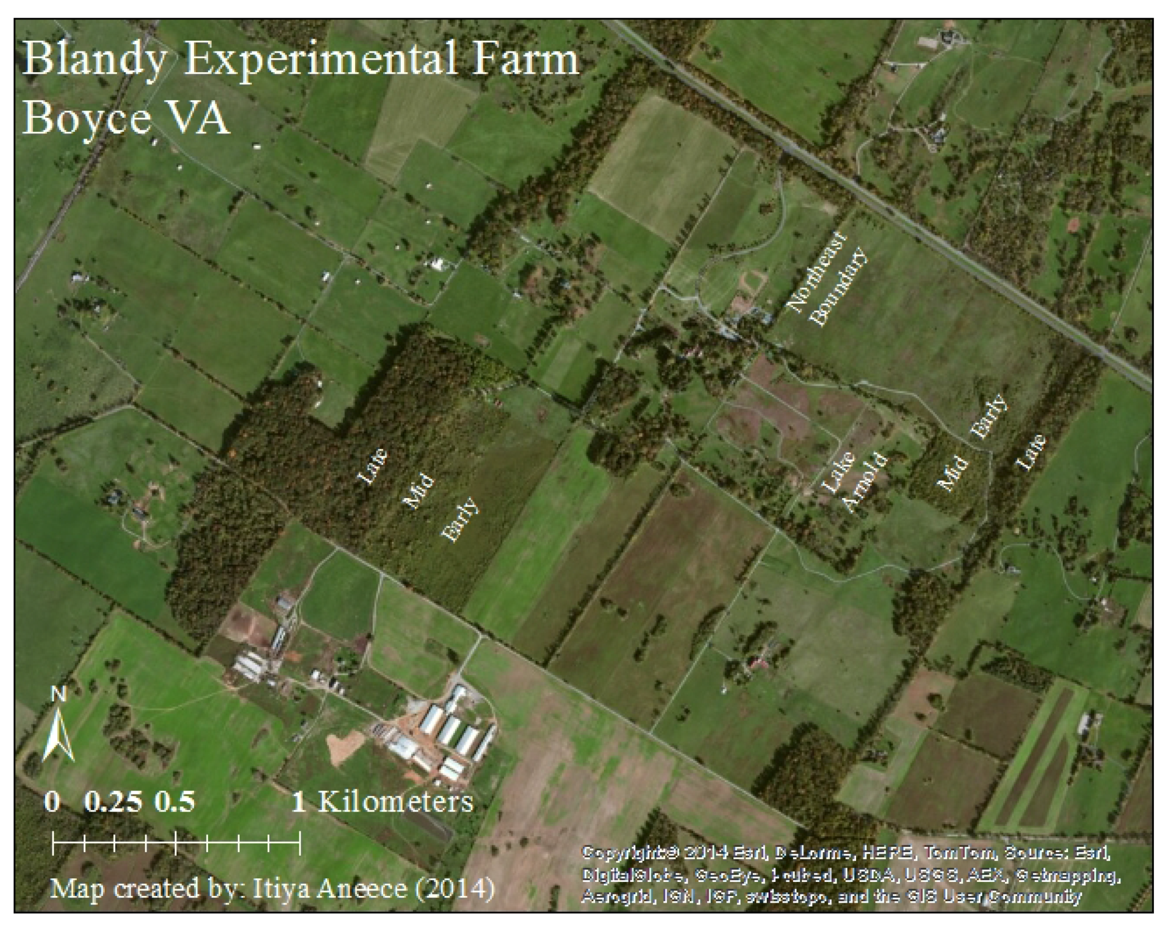
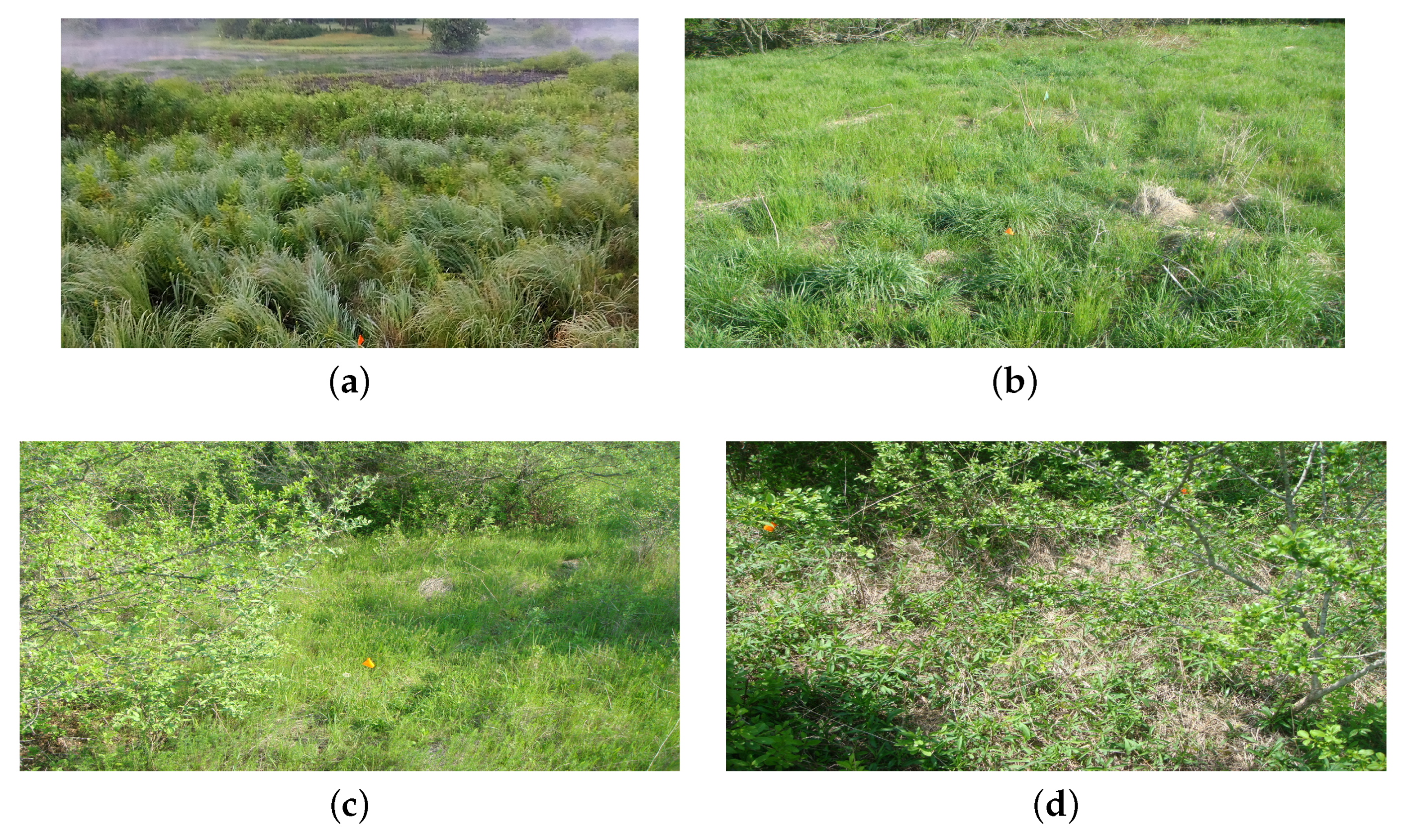
2.1. Study Site

The Blandy Experimental Farm (BEF) (Figure 1), located in the Shenandoah Valley in Clarke County Virginia at 39°09’N, 78°06’W [34], is a 300 ha biological field station owned by the University of Virginia since 1926 and operated by the Department of Environmental Sciences since 1983 [35]. The BEF contains 120 ha of pasture and cropland, 40 ha of woodland, the 60 ha Virginia State Arboretum, and 80 ha of old fields in early, middle, and late succession [35]. Each of two successional series (southwest and northeast) contains an early, mid, and late successional field. The successional fields are former agricultural fields, abandoned in 2001 (Early 1), 2003 (Early 2), 1986 (Mid 1), 1987 (Mid 2), before 1910 (Late 1) and before 1920 (Late 2) [1]. Two additional field sites were considered alongside the successional field chronosequences: near Lake Arnold and a site at a field boundary near the northeast successional series. Soils are deep colluvial and alluvial sediment from karst limestone, shale, and siltstone; study sites have well-drained silt loam soil, of the soil Order Ultisol, with slopes less than 10% [35]. With an elevation of 190 m, the BEF has a mean annual temperature and precipitation of 11.8 °C and 940 mm respectively, an average growing season of 157 days, and average annual primary productivity of 1.0 kg·m−2 in the successional fields [1,35]. The exotic invasive species that occupy these fields at BEF have several traits that assist their establishment and spread, and thus affect community composition (see Appendix, Persistence of invasive plants).
Figure 1. Blandy Experimental Farm, Boyce VA with study site labels including two secondary successional fields.
Remotesensing 07 15850 g001

2.2. Field Methods

To discriminate plant communities using hyperspectral remote sensing, three 5 m × 5 m community-level plots were established in the summer of 2014 in each of four sites at the BEF: Lake Arnold (LA), the northeast boundary (NEB), and the early successional stage in both the northeast (NEE) and southwest (SWE) successional chronosequences for a total of 24 plots. Only early stages from the successional series were used for ground-level spectral analyses (Figure 2) because of vegetation height in later successional stages. From these plots, using a PANalytical Analytical Spectral Devices (ASD) Inc. (Boulder, CO, USA) FieldSpec® 3 with a 25° field of view (FOV), we collected community-level spectra in the summer of 2014. Hyperspectral reflectance measurements from 350 nm to 1025 nm were collected from approximately 2.5 m in height for a measurement footprint of approximately 1.15 m in diameter. We accomplished this by standing on a stool and using a custom-made polyvinyl chloride (PVC)-pipe extension holding the pistol grip to avoid any spectral signature from the stool or observer. We collected spectra in a way that maximized coverage without trampling vegetation, taking measurements in each corner of the plot, in the center, and the middle of each edge for a total of 12 spectral footprints per plot with each footprint capturing a subsample of the community (Figure 3). Approximately three spectral samples were collected for each spectral footprint for a total of around 36 spectra per plot (Table 1), and spectral measurements were averaged by footprint. We measured the location of the center of each footprint using a plumb-line for several plots and calculated the average location for each footprint in the grid. Spectra were taken during cloud-free days between 10 AM and 2 PM during peak growing season (July) to minimize diurnal and seasonal variability and minimize soil signatures; the spectroradiometer was calibrated at approximately 10 min intervals using a Spectralon white reference panel and dark current measurements. We also conducted vegetation surveys on the 5 m × 5 m grids at 0.5 m intervals, recording species at the ground level, sub-canopy, and canopy to assess species composition of the spectral footprints. Grids were established using PVC pipes to mark the periphery of the 5 m × 5 m plots. Pipes had holes drilled at 0.5 m intervals; a string with hooks on either end was then moved along the pipes, using holes as anchors. The string had knots at 0.5 m intervals, and plants were surveyed at the knots. Therefore, we were able to map the gridpoints that fell within each footprint, using the footprint centers measured with the plumb-line, and know which species were encompassed within each footprint.
Figure 2. Examples of early-stage community plots from (a) Lake Arnold; (b) the northeast boundary; (c) the Northeast chronosequence; and (d) the Southwest chronosequence.
Remotesensing 07 15850 g002
Figure 3. Layout of 5 m × 5 m community-plots. Circles represent spectral footprints taken from outside the plots so as not to trample vegetation. Vegetation surveys were conducted at each 0.5 m interval within a plot for a total of 121 points at the ground, understory, and canopy level.
Remotesensing 07 15850 g003
Table 1. Number and date of community spectra collected; no species-level spectra were used for this study. Signatures were collected in a two-day period during peak growing season to minimize seasonal variability and soil signature while providing a fair comparison across plant communities.
PlotNumber of SpectraDate of Collection
lacp1375 July 2014
lacp2365 July 2014
lacp3365 July 2014
nebcp1364 July 2014
nebcp2364 July 2014
nebcp3364 July 2014
neecp1374 July 2014
neecp2374 July 2014
neecp3364 July 2014
swecp1355 July 2014
swecp2365 July 2014
swecp3385 July 2014

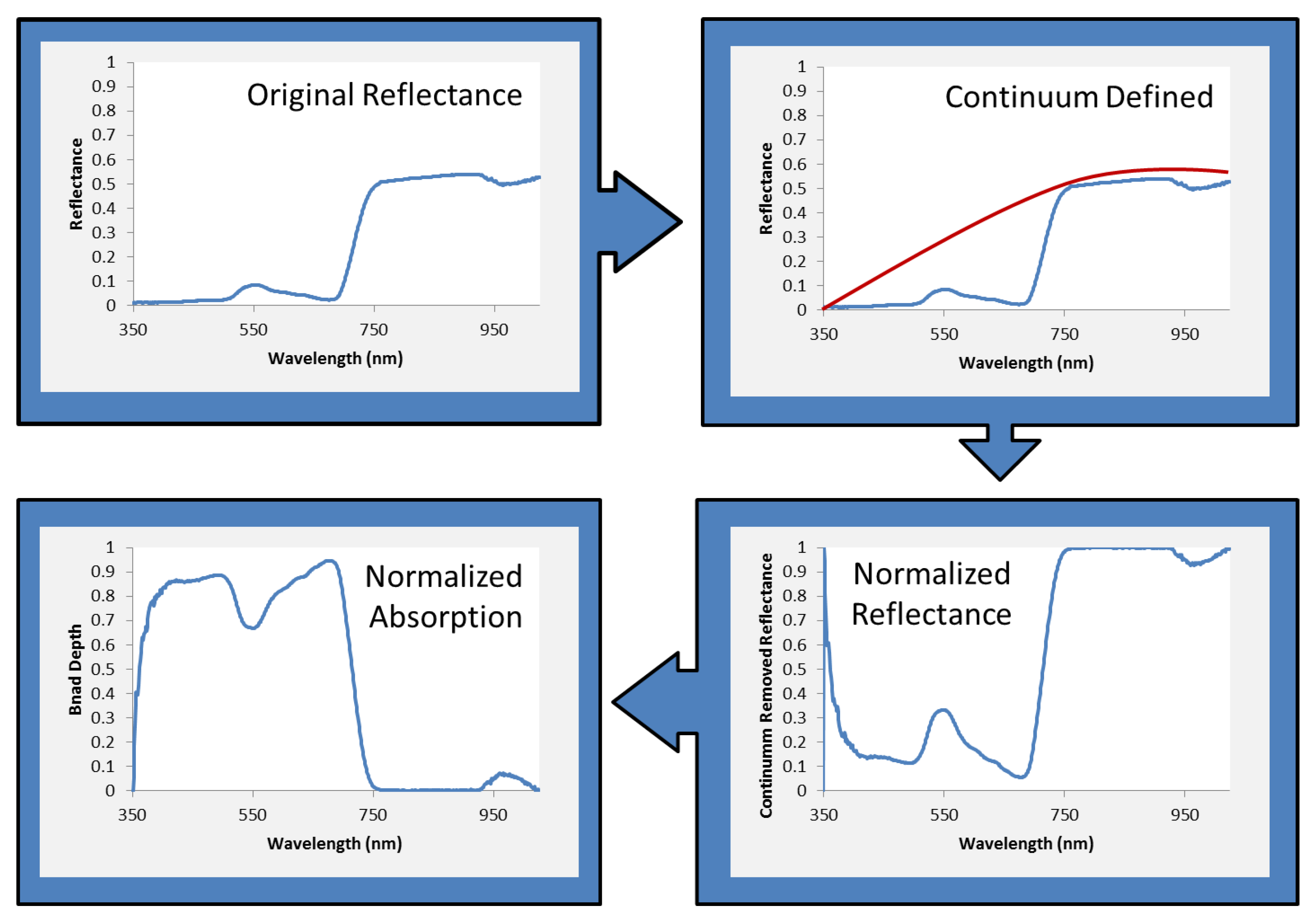
2.3. Data Analysis and Statistical Methods

To minimize any atmospheric and soil noise in the spectral data, we calculated band depth from original reflectance profiles, and this band depth profile was used for subsequent analysis. To obtain band depth, a continuum hull was matched to the original spectral profile, and this continuum was removed from the original spectral profile to get normalized reflectance; we then subtracted these continuum-removed reflectance values from one to get the band depth profile. An example of this calculation is illustrated using an average buckthorn spectral profile (Figure 4). The continuum hull is comprised of several lines connecting local maxima and has been used by many researchers to minimize noise, increase discriminability, and increase accuracy in estimating physiological characteristics [17,36,37]. For more information on continuum removal, refer to Schmidt and Skidmore [38] and Clark and Roush [39].
Figure 4. Calculating band depth (normalized absorption) from original reflectance using continuum removal.
Remotesensing 07 15850 g004
Vegetation survey data were matched to footprints used for spectral data collection using the grid points that fell within the footprints. To determine discriminability among communities using community-plot spectra and vegetation surveys, we used PC-ORD (Version 6, MjM Software, Gleneden Beach, OR, USA) to conduct multivariate non-metric multidimensional scaling (NMS) ordination analyses. This analysis orients samples in an ordination space based on the similarities between samples [40]. We used this technique, along with Bray-Curtis distance, to determine clustering of footprints within plots, by species compositions. Subsequently, we ran a stepwise regression in SAS (Statistical Analysis Software, Version 9.4, SAS Institute Inc., Cary, NC, USA) to examine which species most influenced the ordination axes and thus plot footprint clustering, considering species with a significance level of p < 0.0001.
We ran a similar ordination analysis using footprint-level spectral data to assess spectral clustering of plot footprints, followed by a multiple regression to examine which wavelengths most influenced clustering. To reduce correlation among wavelengths prior to running the regression analysis, we performed a principal components analysis (PCA) in SAS to select uncorrelated wavelengths that explained most of the variability in the dataset; this was done by selecting wavelengths with the greatest absolute value of factor loadings. The regression then used these wavelengths to assess which most influenced the ordination axes. We also assessed the relationships between species ordination axis loadings and band depth axis loadings to determine whether certain species may be associated with certain spectral characteristics.
To determine whether we could use spectral data to differentiate among plots and whether the use of multiple narrow bands would increase discriminability, we ran two discriminant analyses (DA). One used seven simulated broad bands corresponding with those of WorldView2, and another used wavelengths selected from the PCA. The WorldView2 bands were simulated using the reflectance spectra, averaging 400–449 nm, 450–509 nm, 510–580 nm, 585–625 nm, 630–690 nm, 705–745 nm, and 770–895 nm. The eighth WorldView2 band of 860–1040 nm extends past the wavelengths measured using the FieldSpec3, and thus was not simulated. User’s, producer’s, and overall accuracies were calculated, along with the Matthew’s Correlation Coefficient (MCC, Equation (1), where TP = True Positive, TN = True Negative, FP = False Positive, and FN = False Negative) to test for reliability. MCC values range from 1 to −1, where 1 represents perfect predictability, 0 represents predictability as good as random, and −1 represents predictability exactly opposite of expected.
M C C = T P * T N - F P * F N T P + F P * T P + F N * T N + F P * T N + F N

3. Results and Discussion

In this study, we asked whether plant communities could be distinguished spectrally, and which species and spectral attributes were most useful for discrimination. Species composition differed by field, as found through vegetation surveys and species ordination results, and these differences were observed spectrally using ordinations of band depth data. Using the bands selected by the PCA in a discriminant analysis, plots within fields were not as readily distinguished as plots across fields, perhaps because of greater similarities in species compositions within fields than between fields. Nevertheless, plots were able to be separated more successfully using narrow bands derived from hyperspectral data than by using simulated WorldView2 broad bands.

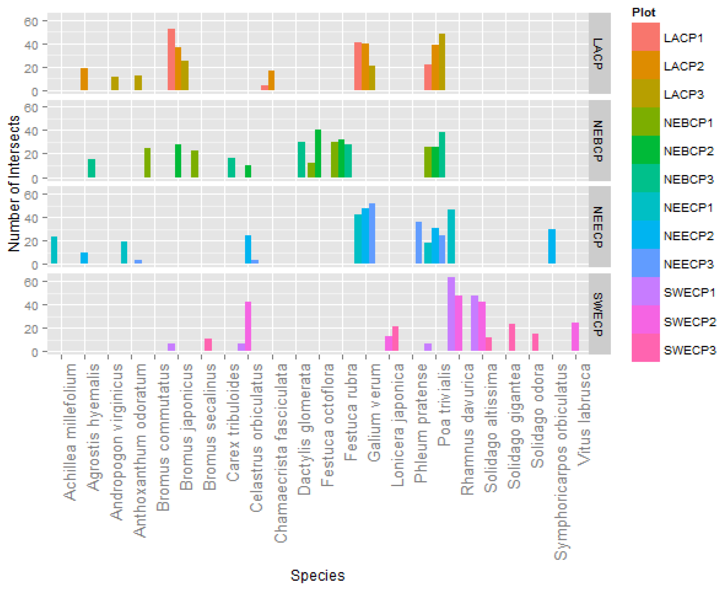
3.1. Species Ordinations
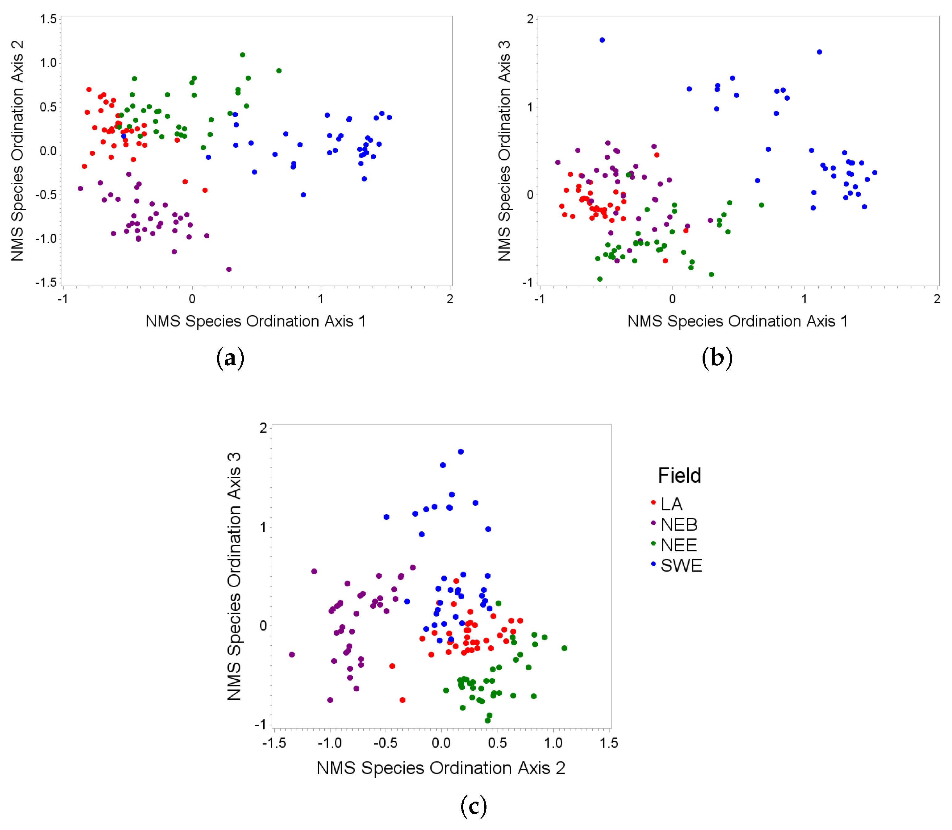
Species compositions differed by fields and by plots within fields (Figure 5). Lake Arnold (LA) plots predominantly consisted of Galium verum (yellow bedstraw), Poa trivialis (rough bluegrass), and Bromus japonicus (Japanese brome). In the northeast boundary (NEB), plots were dominated by grass species including Poa trivialis, Festuca rubra (red fescue), and Festuca octoflora (sixweek fescue). The northeast early (NEE) successional plots consisted mostly of Galium verum, Poa trivialis, and Rhamnus davurica (Dahurian buckthorn). The southwest early (SWE) plots mostly contained Rhamnus davurica, Solidago altissima (tall goldenrod), and Celastrus orbiculatus (oriental bittersweet) (Figure 5).
Figure 5. Species composition from vegetation surveys of community plots (CP) at Blandy Experimental Farm in northern Virginia at Lake Arnold (LA), the boundary near the northwest successional field (NEB), the northeast early successional seres (NEE), and the southwest early successional seres (SWE), where the y-axis represents the number of intersects (out of the total 121 intersects surveyed in each plot) at which certain species were found.
Remotesensing 07 15850 g005
These differences in species compositions were demonstrated in the ordination results as footprints clustered by plot and by field in ordination space (Figure 6). Hence, species compositions were similar within plots and within fields. The species that most influenced axis 1 of the composition ordination were Solidago altissima (tall goldenrod) and Bromus japonicus (Japanese brome), while axis 2 was most influenced by Festuca rubra (red fescue), Galium verum (yellow bedstraw), Muhlenbergia schreberi (nimblewill), Achillea millefolium (yarrow), and Bromus commutatus (meadow brome). Axis 3 was most influenced by Galium verum (yellow bedstraw), Solidago gigantea (giant goldenrod), Dactylis glomerata (orchard grass), Bromus japonicus (Japanese brome), Ambrosia artemisiifolia (common ragweed), and Lonicera japonica (Japanese honeysuckle) (Table 2).
Many of the species that most influenced the ordination axes were also dominant in the community plots, especially in a particular field, making them important for discriminating across fields. As examples, S. altissima was dominant in the SWE plots, F. rubra was dominant in the NEB plots, and G. verum was dominant in the LA and NEE plots. These three species were influential to axes 1, 2, and 3 respectively in the species ordinations.
As we had surmised, many of the most influential species are also considered invasive, including Festuca rubra, Galium verum, Muhlenbergia schreberi, Achillea millefolium, Dactylis glomerata, Ambrosia artemisiifolia, and Lonicera japonica [41,42]. This supports the idea that these invasive species affect community composition, and likely community properties as well. Additionally, subordinate species may be important determinants of ecosystem function because they can influence which species become dominant and may themselves become dominant if current dominants are suppressed [43]. Thus, invasive species might have effects on ecosystem function and community composition even at low densities.
Figure 6. Non-metric multidimensional scaling (NMS) ordination results using species composition from Lake Arnold (LA), northeast boundary (NEB), northeast early (NEE), and southwest early (SWE) fields at the Blandy Experimental Farm in northern Virginia for (a) axes 1 and 2; (b) axes 1 and 3; and (c) axes 2 and 3.
Remotesensing 07 15850 g006
Table 2. Stepwise regression results on which species most influence non-metric multidimensional scaling (NMS) ordination axes. Enough species were retained to have a cumulative R2 of 0.80. All species indicated here are significant to p < 0.0001.
AxisSpeciesPartial R-Square
Axis 1Solidago altissima0.6962
Axis 1Bromus japonicus0.1117
Axis 2Festuca rubra0.5538
Axis 2Galium verum0.1251
Axis 2Muhlenbergia schreberi0.0737
Axis 2Achillea millefolium0.0433
Axis 2Bromus commutatus0.0363
Axis 3Galium verum0.3817
Axis 3Solidago gigantea0.2266
Axis 3Dactylis glomerata0.0813
Axis 3Bromus japonicus0.0573
Axis 3Ambrosia artemisiifolia0.0476
Axis 3Lonicera japonica0.0336

3.2. Spectral Ordinations

Footprint similarities were also assessed using spectral data; we again found clustering of footprints by plot and by field (Figure 7). Before running a regression analysis to determine which bands most influenced NMS ordination axis values, a segmented principal components analysis (PCA) was conducted; the wavelengths selected, based on the greatest absolute value of factor loadings, were 435 nm, 525 nm, 575 nm, 635 nm, 680 nm, 710 nm, 750 nm, 835 nm, and 970 nm. Band depths at these wavelengths were entered into a regression analysis to determine which wavelengths most explained the ordination axes; these wavelengths were 435 nm, 635 nm, 680 nm, 710 nm, 750 nm, and 970 nm for axis 1; 435 nm, 525 nm, 575 nm, 635 nm, 750 nm, 970 nm for axis 2; and 525 nm, 575 nm, 635 nm, 710 nm, 750 nm, and 835 nm for axis 3 (Table 3).
Figure 7. Non-metric multidimensional scaling (NMS) ordination results using band depth values from Lake Arnold (LA), northeast boundary (NEB), northeast early (NEE), and southwest early (SWE) fields at the Blandy Experimental Farm in northern Virginia for (a) axes 1 and 2; (b) axes 1 and 3; and (c) axes 2 and 3.
Remotesensing 07 15850 g007
Table 3. Multiple regression coefficients, assessing which wavelengths most influence non-metric multidimensional scaling (NMS) ordination axes.
Axis435525575635680710750835970
Axis 13.60..7.40−7.66−4.781.78.8.48
Axis 26.31−1.653.447.28..2.86.2.22
Axis 3.−4.116.96−6.41.3.795.315.59.
The wavelengths selected through the principal components analysis (PCA) as most encompassing variability across plots were 435, 525, 575, 635, 680, 710, 750, 835, and 970 nm. The entire spectral profile was represented, because we used a segmented PCA rather than using the entire spectral profile. This is important because of the differences in magnitudes of reflectance values along the spectral profile; the greater the reflectance value at a particular wavelength, the more likely that wavelength may be to influence a principal component. Using the segmented PCA allows for the representation of biologically meaningful features across the entire spectral profile. As examples, the reflectance values at 435 nm and 575 nm are influenced by carotenoids and chlorophyll more so than by anthocyanins [44,45]. At 525 nm, there is more influence by anthocyanins than carotenoids and chlorophylls [44,45]. Chlorophylls a and b have peaks near 680 and 635 nm, respectively [44,45]. Wavelengths in the red edge such as 710 nm and 750 nm can be used to estimate chlorophyll content because they are less affected by leaf structure and canopy structure [46]. The near-infrared bands, such as 835 nm, have been used to assess leaf structure [47]. The water absorption feature near 970 nm is often used to estimate leaf water content [48]. Using these wavelengths, a discriminant analysis was successfully used to distinguish among communities. The DA revealed that there was high discriminability across fields, but less discriminability within fields; this is consistent with greater species composition similarity across than within fields.
Within the band depth ordination results, axis 1 was positively influenced by band depth at 435, 635, 750, and 970 nm and negatively influenced by band depth at 680 and 710 nm. Spectra with high axis 1 values are characterized by (1) having high absorption associated with carotenoids and chlorophyll (chl), especially chl b over chl a; (2) having a less steep red edge; and (3) having a large water absorption feature at 970 nm. Axis 2 was positively influenced by 435, 575, 635, 750, and 970 nm and negatively influenced by 525 nm. Thus, spectra with high axis 2 values are characterized by high absorption associated with carotenoids and chlorophylls, especially chl b, and not by anthocyanins; they also have high absorption at the red-edge shoulder and a large water absorption feature at 970 nm. Axis 3 was positively associated with 575, 710, 750, and 835 nm and negatively associated with 525 and 635 nm. Spectra with high axis 3 values are characterized by high absorption associated with carotenoids and chl a, but not by chl b or anthocyanins; they have high absorptions in the near-infrared plateau.
To determine whether these spectral characteristics may be correlated with certain species, the species ordination axis loadings were assessed for correlations with band depth loadings. There were positive correlations between species axis 1 and band depth axis 1 (r = 0.513, p < 0.0001) and between species axis 1 and band depth axis 2 (r = 0.718, p < 0.0001). There was a negative correlation between species axis 2 and band depth axis 3 (r = −0.450, p < 0.0001). The species that were most strongly correlated with axis 1 in the species ordinations were S. altissima and B. japonicus. These species may be characterized by higher absorption by carotenoids and chl b than by anthocyanins and chl a; they also may have high absorption in the red-edge shoulder region and the water absorption feature at 970 nm. The species associated with axis 2 may be characterized by greater absorption due to anthocyanins and chl b, and higher reflectance in the red edge and near-infrared regions. However, caution must be used in analyzing these composite spectra, since features from multiple species are being expressed within one spectral profile.

3.3. Discriminant Analyses

There was high separability among fields, but low separability among plots using simulated WorldView2 broad bands (Table 4). As an example, 32 out of 36 NEB spectra were correctly identified as NEB, but only 16 out of those 32 were identified as the correct plot within NEB. Similarly, 32 out of 36 SWE spectra were correctly identified as SWE, but only 22 out of those 32 were identified as the correct SWE plot.
In contrast, using multiple narrowband wavelengths selected by the PCA in a discriminant analysis, we found greater spectral separability of plots (Table 5). As an example, 33 out of 36 NEB spectra were correctly identified as NEB, and 27 out of those 33 were identified as the correct NEB plot. Similarly, 35 out of 36 SWE spectra were correctly identified as SWE, and 31 out of those 35 were identified as the correct SWE plot. User’s, producer’s, and overall accuracies and the MCC values were greater using narrow bands than using simulated broad bands (Table 6).
Table 4. Confusion matrix for summer 2014 discriminant analysis to test discriminabilty of plots using 7 simulated WorldView2 bands: 400–449, 450–509, 510–580, 585–625, 630–690, 705–745, and 770–895 nm.
Number of Observations Classified into Plot
lacp1lacp2lacp3nebcp1nebcp2nebcp3neecp1neecp2neecp3swecp1swecp2swecp3TotalProducer’s Accuracy
lacp112000000000001285.7%
lacp2012000000000012100%
lacp32080010001001288.9%
nebcp10004520100001244.4%
nebcp20004620000001246.2%
nebcp30001260021001254.5%
neecp10000004322101244.4%
neecp20010003610011240.0%
neecp30000002370001250.0%
swecp10000000115141245.5%
swecp20000000002821272.7%
swecp30000000110191256.3%
Total141299131191514111116144
User’s Accuracy100%100%66.7%33.3%50.0%50.0%33.3%50.0%58.3%41.7%66.7%75.0%
Overall Accuracy 60.4%
Table 5. Confusion matrix for summer 2014 discriminant analysis to test discriminabilty of plots using wavelengths selected using principal components analysis: 435, 525, 575, 635, 680, 710, 750, 835, 970 nm.
Number of Observations Classified into Plot
lacp1lacp2lacp3nebcp1nebcp2nebcp3neecp1neecp2neecp3swecp1swecp2swecp3TotalProducer’s Accuracy
lacp111100000000001278.6%
lacp211010000000001283.3%
lacp32170020000001277.8%
nebcp10008300010001288.9%
nebcp200011010000001271.4%
nebcp30010190010001275.0%
neecp10000008012011280.0%
neecp20000001700041277.8%
neecp300000011100001277.0%
swecp100000000011101273.3%
swecp20000000002911290.0%
swecp300000001000111264.7%
Total141299141210913151017144
User’s Accuracy91.7%83.3%58.3%66.7%83.3%75%66.7%58.3%83.3%91.7%75.0%91.7%
Overall Accuracy 77.1%
Table 6. A comparison of discrimination accuracies and reliability using simulated WorldView2 broad bands, and narrow bands from hyperspectral field-measurements.
Simulated Broad BandsNarrow Bands
Matthew’s Correlation Coefficient0.5480.745
Overall Accuracy60.4%77.1%
Average Producer’s Accuracy60.7%78.1%
Average User’s Accuracy60.4%77.1%
Therefore, plant communities may be more successfully discriminated spectrally using narrow bands than broad bands. Additionally, the narrow band values entered into the discriminant analysis were band depth rather than reflectance values, which may also have contributed to the increase in discriminability.

3.4. Other Considerations

The spectral differences between fields may also have been due to differences in soil characteristics among fields. If soil signatures were a large part of the spectral footprints (i.e., for small-leaved species), these differences in soil signatures in the plots and fields may contribute to the spectral differences in plots and fields. Depending on vegetation cover, differences in soil moisture and soil texture can influence spectral data [16,49,50]. Differences in soil characteristics such as soil nutrients, soil biota, and soil pH could also directly and indirectly influence differences observed among communities [51]. Land use can influence soil characteristics [52] and species composition [13,53,54]. The four fields studied at the Blandy Experimental Farm differ in land use history [1] and in soil characteristics. Therefore, it is important to take land use history into account when studying invaded systems [55,56] and secondary successional systems [54,57]. Additionally, species composition can influence soil characteristics by mechanically changing the soil, affecting nutrient cycling, altering soil biota, and by changing herbivore community compositions [5,58].
As another consideration, band depth may not always be the best way to normalize data and correct for noise although it is quite commonly used [32,48,59,60]. Additional techniques for extracting spectral information include the use of first and second derivatives [61,62], and band ratios [63,64]. Band depth, however, is widely used to estimate vegetation water, nitrogen, lignin, and cellulose content [32,48] and to discriminate among minerals [59,60], because it reduces the effects of sensor noise, atmospheric effects, background soil signatures, and variations in topography and albedo [32,59]. However, the output of this procedure varies depending on the range over which the continuum is established. Band depth might also not be the most useful technique for all parts of the spectral profile. Therefore, another noise minimization technique may be better able to preserve information from the original reflectance spectral profile, for example, in the near-infrared region where differences are often dampened by band depth calculations.
Additionally, only early-stage spectral signatures were analyzed in this study due to the height of the vegetation. Therefore, the separability of plant communities in the early stages could not be compared with separability of plant communities at mid and late stages. Future research with satellite or airborne imagery could help rectify this short-coming; however, the differences in remote-sensing platforms, such as spatial and spectral resolutions, would need to be taken into account. Further research could also be done to assess discriminability across plant communities early and late in the growing season, but at these times the soil signature may inhibit discrimination; senescence during late stages of the growing season could also inhibit discriminability.

3.5. Context of Key Findings

Overall, we were able to visualize and analyze differences in communities by species composition using ordination analyses. Schmidtlein et al. [40] used NMS ordinations to study undefined vegetation assemblages and used partial least squares regression analysis to assess which bands were most influential to the assemblages. Similarly, we used regressions to determine the most influential species to clustering: Solidago altissima (tall goldenrod), Bromus japonicus (Japanese brome), Festuca rubra (red fescue), Galium verum (yellow bedstraw), Muhlenbergia schreberi (nimblewill), Achillea millefolium (yarrow), Bromus commutatus (meadow brome), Solidago gigantea (giant goldenrod), Dactylis glomerata (orchard grass), Ambrosia artemisiifolia (common ragweed), and Lonicera japonica (Japanese honeysuckle). Several of these species are considered invasive in Virginia (F. rubra, G. verum, M. schreberi, A. millefolium, D. glomerata, A. artemisiifolia, and L. japonica), illustrating how invasive species can influence community composition [41].
We were also able to spectrally separate communities using ordinations. Gao and Zhang [65] also examined such differences in vegetation, using ground-level spectral data to discriminate salt marsh communities. These spectral differences by communities may be due to differences in species-level characteristics since the reflectance in the visible region is influenced by pigment concentration and reflectance in the near-infrared region is influenced by leaf structure [26], and these characteristics can differ by species. This idea was supported when we used regressions to determine the most influential wavelengths for clustering of communities: 435, 525, 575, 635, 680, 710, 750, 835, and 970 nm. These wavelengths are representative of absorption by pigments, leaf structure, and leaf water content; such features differ by species and by communities that differ in species composition.
Similar spectral features have been used to discriminate among species [17,21,22,23,24,25]. If such features are able to be detected at the satellite level, discriminability may also be possible using satellite imagery. Since the most readily available satellite data are multispectral with medium or coarse spatial resolution, this may be challenging considering the lower discriminability we observed using simulated broad bands. However, discriminability may become easier with the advances in hyperspectral satellite technology such as the existing Hyperion and future EnMAP and HyspIRI satellites. The German EnMAP (Environmental Mapping and Analysis Program) satellite mission aims to use a pushbroom sensor to collect visible, near infrared, and shortwave infrared (420 nm–2450 nm) reflectances with 244 bands, high radiometric resolution of 14 bits, a spatial resolution of 30 m, and a 30° off-nadir pointing feature and sun-synchronous orbit that will allow a four-day temporal resolution; it is scheduled to launch around 2018 [66]. Additionally, the HyspIRI (Hyperspectral Infrared Imager) mission, scheduled to launch by 2022, will have two instruments on a satellite in Low Earth Orbit that will collect reflectance measurements from 380 nm to 2500 nm and 3 μm to 12 μm with a spatial resolution of 60 m and revisit times of 19 days for visible to shortwave regions and five days for thermal infrared [67]. Advances in high spatial resolution satellites, such as the WorldView2 and WorldView3 satellites with resolutions of 1.84 m and 1.24 m respectively for multispectral bands, would also increase species discriminability with the reduction of spectral mixing; WorldView3 also has decent spectral resolution, with 16 bands from the visible to shortwave-infrared regions. Using hyperspectral and high-spatial resolution data to monitor plant communities and how they may be affected by invasion at large spatial extents can aid conservation efforts and help us preserve the biodiversity that is associated with ecosystem function.

4. Conclusions

We were able to distinguish among plant communities that differed in species compositions using ground-level hyperspectral remote sensing data. Seven of the eleven most influential species in defining these plant communities are considered invasive in Virginia, demonstrating the impact of invasive species on community composition. Plant communities were more accurately discriminated amongst using narrow bands than by using simulated broad bands, with a 77% overall accuracy versus 60% percent. Thus, narrow bands provide improved accuracies relative to broad bands in the study of plant communities, perhaps because narrow bands provide useful details that may be averaged out by broad bands. In this study, we demonstrated that we could discriminate among early successional plant communities using remote sensing data collected at the ground-level. Further work could be done using airborne or satellite imagery in mid and late successional stages to observe plant community discriminability at larger spatial extents. However, challenges to this include spatial and spectral resolutions most commonly available in airborne and satellite imagery. Such research will become more feasible with advances in satellite technology, such as the upcoming hyperspectral EnMAP and the available hyperspatial WorldView3 satellites.

Acknowledgments

We would like to thank the University of Virginia and the Blandy Experimental Farm for funding this research. We also thank Jennie Moody, Laura Galloway, Dave Carr, and Clay Ford for advice on experimental design and statistical analyses. We also thank the reviewers for their insightful and constructive comments.

Author Contributions

Itiya Aneece and Howard Epstein designed the study. Itiya Aneece collected and analyzed data. Itiya Aneece and Howard Epstein worked on the paper.

Conflicts of Interest

The authors declare no conflict of interest. The funding sponsors had no role in the design of the study; in the collection, analysis, or interpretation of the data; in the writing of the manuscript, and in the decision to publish the results.

Appendix. Persistence of Invasive Plants

The non-native invasive plant species in this paper have several traits that allow them to persist in and take over a region. As examples, Carduus acanthoides (spiny plumeless thistle) has numerous, though not persistent, seeds [68], is tolerant to repeated disturbances [69], and is opportunistic in colonizing gaps [70]. Rhamnus cathartica (Common buckthorn) has high shade tolerance, high growth and photosynthesis rates, wide range of tolerance of moisture and drought, unique leaf phenology, high fecundity, bird-dispersal of fruit, high germination rate, high seedling success in disturbed sites, and secondary metabolites, especially emodin, which may protect the plant from herbivores, pathogens, and high light levels; emodin may have allelopathic effects on natives nearby, and affect soil microbes and unripe fruit consumption/digestion by birds [71]. Celastrus orbiculatus (Oriental bittersweet) sprawls over or twines around and into the canopy of surrounding vegetation and has low palatability [72]. It does not have a host preference [73]. It can also persist at low photosynthetic rates in the shade and respond quickly to increases in light penetration to outgrow competition even in mature forests [72], is able to spread substantially within the canopy and decrease tree growth after gap-formation [74]. Oriental bittersweet can outcompete American bittersweet due to greater tolerance to various environmental conditions (e.g., shade), faster growth and reproduction rates, ability to increase photosynthetic rates with increases in light, perhaps the ability to perceive and grow toward nearby vegetation that it could then climb [72], a shorter juvenile period, and greater seed viability [75]. In addition to changing species composition of plants, these invasive species can also be host to other types of organisms that could, in turn, affect other plants; buckthorn is the primary overwintering host for soybean aphids, Aphis gossypii and A. glycines [76,77], and oriental bittersweet is host for the bacterim Xylella fastidiosa, which, in turn, infects crop plants [72].

References

  1. Wang, J.; Epstein, H.; Wang, L. Soil CO2 flux and its controls during secondary succession. J. Geophys. Res. 2010, 115. [Google Scholar] [CrossRef]
  2. Mosher, E.; Silander, J.; Latimer, A. The role of land-use history in major invasions by woody plant species in the northeastern North American landscape. Biol. Invasions 2009, 11, 2317–2328. [Google Scholar] [CrossRef]
  3. Chapin, S., III; Walker, B.; Hobbs, R.; Hooper, D.; Lawton, J.; Sala, O.; Tilman, D. Biotic control over the functioning of ecosystems. Science 1997, 277, 500–504. [Google Scholar] [CrossRef]
  4. Kuhman, T.; Pearson, S.; Turner, M. Agricultural land-use history increases non-native plant invasion in a southern Appalachian forest a century after abandonment. Can. J. For. Res. 2011, 41, 920–929. [Google Scholar] [CrossRef]
  5. DeMeester, J.; DeB Richter, D. Differences in wetland nitrogen cycling between the invasive grass Microstegium vimineum and a diverse plant community. Ecol. Appl. 2010, 20, 609–619. [Google Scholar] [CrossRef] [PubMed]
  6. Sullivan, J.; Williams, P.; Timmins, S. Secondary forest succession differs through naturalised gorse and native kanuka near Wellington and Nelson. N. Z. J. Ecol. 2007, 31, 22–38. [Google Scholar]
  7. Yoshida, K.; Oka, S. Invasion of Leucaena leucocephala and its effects on the native plant community in the Ogasawara (Bonin) Islands. Weed Technol. 2004, 18, 1371–1375. [Google Scholar] [CrossRef]
  8. Feldpausch, T.; Rondon, M.; Fernandes, E.; Riha, S.; Wandelli, E. Carbon and nutrient accumulation in secondary forests regenerating on pastures in central Amazonia. Ecol. Appl. 2004, 14, 164–176. [Google Scholar] [CrossRef]
  9. Kassi N’Dja, J.; Decocq, G. Successional patterns of plant species and community diversity in a semi-deciduous tropical forest under shifting cultivation. J. Veg. Sci. 2008, 19, 809–820. [Google Scholar] [CrossRef]
  10. Otto, R.; Krusi, B.; Burga, C.; Fernandez-Palacios, J. Old-field succession along a precipitation gradient in the semi-arid coastal region of Tenerife. J. Arid Environ. 2006, 65, 156–178. [Google Scholar] [CrossRef]
  11. Cunard, C.; Lee, T. Is patience a virtue? Succession, light, and the death of invasive glossy buckthorn (Frangula alnus). Biol. Invasions 2009, 11, 577–586. [Google Scholar] [CrossRef]
  12. Simberloff, D. Invasions of plant communities—More of the same, something very different, or both? Am. Midl. Nat. 2010, 163, 220–233. [Google Scholar] [CrossRef]
  13. Grau, H.R.; Arturi, M.F.; Brown, A.D.; Acenolaza, P.G. Floristic and structural patterns along a chronosequence of secondary forest succession in Argentinean subtropical montane forests. For. Ecol. Manag. 1997, 95, 161–171. [Google Scholar] [CrossRef]
  14. Leicht-Young, S.A.; O’Donnell, H.; Latimer, A.M.; Silander, J.A. Effects of an invasive plant species, Celastrus orbiculatus, on soil composition and processes. Am. Midl. Nat. 2009, 161, 219–231. [Google Scholar] [CrossRef]
  15. Wilfong, B.; Gorchov, D.; Henry, M. Detecting an invasive shrub in deciduous forest understories using remote sensing. Weed Sci. 2009, 57, 512–520. [Google Scholar] [CrossRef]
  16. Zhang, J.; Rivard, B.; Sanchez-Azofeifa, A.; Castro-Esau, K. Intra- and inter-class spectral variability of tropical tree species at La Selva, Costa Rica: Implications for species identification using HYDICE imagery. Remote Sens. Environ. 2006, 105, 129–141. [Google Scholar] [CrossRef]
  17. Schmidt, K.S.; Skidmore, A.K. Exploring spectral discrimination of grass species in African rangelands. Int. J. Remote Sens. 2001, 22, 3421–3434. [Google Scholar] [CrossRef]
  18. Bradley, B.; Mustard, J. Characterizing the landscape dynamics of an invasive plant and risk of invasion using remote sensing. Ecol. Appl. 2006, 16, 1132–1147. [Google Scholar] [CrossRef]
  19. Smith, A.; Blackshaw, R. Weed: Crop discrimination using remote sensing: A detached leaf experiment. Weed Technol. 2003, 17, 811–820. [Google Scholar] [CrossRef]
  20. Jafari, R.; Lewis, M. Arid land characterisation with EO-1 Hyperion hyperspectral data. Int. J. Appl. Earth Obs. Geoinf. 2012, 19, 298–307. [Google Scholar] [CrossRef]
  21. Burkholder, A. Seasonal Trends in Separability of Leaf Reflectance Spectra for Ailanthus altissima and Four Other Tree Species. Master’s Thesis, Eberly College of Arts and Sciences at West Virginia University, Morgantown, WV, USA, 2010. [Google Scholar]
  22. Narumalani, S.; Mishra, D.; Wilson, R.; Reece, P.; Kohler, A. Detecting and mapping four invasive species along the floodplain of North Platte River, Nebraska. Weed Technol. 2009, 23, 99–107. [Google Scholar] [CrossRef]
  23. Pinard, V.; Bannari, A. Spectroradiometric analysis in a hyperspectral use perspective to discriminate between forest species. In Proceedings of the 2003 IEEE International Geoscience and Remote Sensing Symposium, IGARSS’03, Toulouse, France, 21–25 July 2003; Volume 7, pp. 4301–4303.
  24. Rud, R.; Shoshany, M.; Alchanatis, V.; Cohen, Y. Application of spectral features’ ratios for improving classification in partially calibrated hyperspectral imagery: A case study of separating Mediterranean vegetation species. J. Real-Time Image Process. 2006, 1, 143–152. [Google Scholar] [CrossRef]
  25. Gai, Y.Y.; Fan, W.J.; Xu, X.R.; Zhang, Y.Z. Flower species identification and coverage estimation based on hyperspectral remote sensing data. In Proceedings of the 2011 IEEE International Geoscience and Remote Sensing Symposium (IGARSS), Vancouver, BC, Canada, 24–29 July 2011; pp. 1243–1246.
  26. Xiao, Y.; Zhao, W.; Zhou, D.; Gong, H. Sensitivity analysis of vegetation reflectance to biochemical and biophysical variables at leaf, canopy, and regional scales. IEEE Trans. Geosci. Remote Sens. 2014, 52, 4014–4024. [Google Scholar] [CrossRef]
  27. Mahlein, A. Detection, Identification, and Quantification of Fungal Diseases of Sugar Beet Leaves Using Imaging and Non-Imaging Hyperspectral Techniques. Ph.D. Thesis, Universitats- und Landesbibliothek Bonn, Bonn, Germany, 2011. [Google Scholar]
  28. Merzlyak, M.N.; Gitelson, A.A.; Chivkunova, O.B.; Solovchenko, A.E.; Pogosyan, S.I. Application of reflectance spectroscopy for analysis of higher plant pigments. Russ. J. Plant Physiol. 2003, 50, 704–710. [Google Scholar] [CrossRef]
  29. Buschmann, C.; Nagel, E.; Rang, S.; Stober, F. Interpretation of reflectance spectra of terrestrial vegetation based on specifical plant test systems. In Proceedings of the 10th Annual International Geoscience and Remote Sensing Symposium, IGARSS ’90, College Park, MD, USA, 20–24 May 1990; pp. 1927–1930.
  30. Papes, M.; Tupayachi, R.; Martinez, P.; Peterson, A.; Powell, G. Using hyperspectral satellite imagery for regional inventories: A test with tropical emergent trees in the Amazon Basin. J. Veg. Sci. 2010, 21, 342–354. [Google Scholar] [CrossRef]
  31. Gamon, J.; Berry, J. Facultative and constitutive pigment effects on the Photochemical Reflectance Index (PRI) in sun and shade conifer needles. Isr. J. Plant Sci. 2012, 60, 85–95. [Google Scholar] [CrossRef]
  32. Kokaly, R.; Clark, R. Spectroscopic determination of leaf biochemistry using band-depth analysis of absorption features and stepwise multiple linear regression. Remote Sens. Environ. 1999, 67, 267–287. [Google Scholar] [CrossRef]
  33. Roberts, D.; Ustin, S.L.; Ogunjemio, S.; Greenberg, J.; Dobrowski, S.; Chen, J.; Hinckley, T. Spectral and structural measures of northwest forest vegetation at leaf to landscape scales. Ecosystems 2004, 7, 545–562. [Google Scholar] [CrossRef]
  34. Wang, L.; Shaner, P.; Macko, S. Foliar delta 15N patterns along successional gradients at plant community and species levels. Geophys. Res. Lett. 2007, 34, L16403. [Google Scholar] [CrossRef]
  35. Bowers, M.A. University of Virginia’s Blandy Experimental Farm. Bull. Ecol. Soc. Am. 1997, 78, 220–225. [Google Scholar]
  36. Mitchell, J.; Glenn, N.; Sankey, T.; Derryberry, D.; Germino, M. Remote sensing of sagebrush canopy nitrogen. Remote Sens. Environ. 2012, 124, 217–223. [Google Scholar] [CrossRef]
  37. Sanches, I.; Filho, C.; Kokaly, R. Spectroscopic remote sensing of plant stress at leaf and canopy levels using the chlorophyll 680 nm absorption feature with continuum removal. ISPRS J. Photogramm. Remote Sens. 2014, 97, 111–122. [Google Scholar] [CrossRef]
  38. Schmidt, K.; Skidmore, A. Spectral discrimination of vegetation types in a coastal wetland. Remote Sens. Environ. 2003, 85, 92–108. [Google Scholar] [CrossRef]
  39. Clark, R.; Roush, T. Reflectance spectroscopy: Quantitative analysis techniques for remote sensing applications. J. Geophys. Res. 1984, 89, 6329–6340. [Google Scholar] [CrossRef]
  40. Schmidtlein, S.; Zimmermann, P.; Schupferling, R.; Weiß, C. Mapping the floristic continuum: Ordination space position estimated from imaging spectroscopy. J. Veg. Sci. 2007, 18, 131–140. [Google Scholar] [CrossRef]
  41. EDDMapS. EDDMapS: Early Detection and Distribution Mapping System. Available online: http://www.eddmaps.org/ (accessed on 5 March 2014).
  42. USDA Plants Database. USDA: United States Department of Agriculture, Natural Resources Conservation Services, Plants Database. Available online: http://www.plants.usda.gov/ (accessed on 3 March 2015).
  43. Grime, J. Benefits of plant diversity to ecosystems: Immediate, filter and founder effects. J. Ecol. 1998, 86, 902–910. [Google Scholar] [CrossRef]
  44. Blackburn, G.A. Hyperspectral remote sensing of plant pigments. J. Exp. Bot. 2006, 58, 855–867. [Google Scholar] [CrossRef] [PubMed]
  45. Koning, R. Light Reactions. Plant Physiology Information Website. 1994. Available online: http://plantphys.info/plant_physiology/lightrxn.shtml (accessed on 22 May 2015).
  46. Sims, D.; Gamon, J. Relationships between leaf pigment content and spectral reflectance across a wide range of species, leaf structures and developmental stages. Remote Sens. Environ. 2002, 81, 337–354. [Google Scholar] [CrossRef]
  47. Gamon, J.; Field, C.; Roberts, D.; Ustin, S.; Valentini, R. Functional patterns in an annual grassland during an AVIRIS overflight. Remote Sens. Environ. 1993, 44, 239–253. [Google Scholar] [CrossRef]
  48. Wang, J.; Xu, R.; Yang, S. Estimation of plant water content by spectral absorption features centered at 1450 nm and 1940 nm regions. Environ. Monit. Assess. 2009, 157, 459–469. [Google Scholar] [CrossRef] [PubMed]
  49. Laidler, G.; Treitz, P.; Atkinson, D. Remote sensing of Arctic vegetation: Relations between the NDVI, spatial resolution and vegetation cover on Boothia Peninsula, Nunavut. Arctic 2008, 61, 1–13. [Google Scholar] [CrossRef]
  50. Cochrane, M.A. Using vegetation reflectance variability for species level classification of hyperspectral data. Int. J. Remote Sens. 2000, 21, 2075–2087. [Google Scholar] [CrossRef]
  51. Baron, J.; Barber, M.; Adams, M.; Agboola, J.; Allen, E.; Bealey, W.; Bobbink, R.; Bobrovsky, M.V.; Bowman, W.; Branquinho, C.; et al. The effects of atmospheric nitrogen deposition on terrestrial and freshwater biodiversity. In Nitrogen Deposition, Critical Loads and Biodiversity; Sutton, M., Mason, K., Sheppard, L., Sverdrup, H., Haeuber, R., Hicks, W., Eds.; Springer: Dordrecht, The Netherlands, 2014; pp. 465–480. [Google Scholar]
  52. Castro, H.; Fortunel, C.; Freitas, H. Effects of land abandonment on plant litter decomposition in a Montado system: Relation to litter chemistry and community functional parameters. Plant Soil 2010, 333, 181–190. [Google Scholar] [CrossRef]
  53. Aragon, R.; Morales, J. Species composition and invasion in NW Argentinian secondary forests: Effects of land use history, environment and landscape. J. Veg. Sci. 2003, 14, 195–204. [Google Scholar] [CrossRef]
  54. Riedel, S.; Epstein, H. Edge effects on vegetation and soils in a Virginia old-field. Plant Soil 2005, 270, 13–22. [Google Scholar] [CrossRef]
  55. Rooney, T.; Rogers, D. Colonization and effects of garlic mustard (Alliaria petiolata), European buckthorn (Rhamnus cathartica), and Bell’s honeysuckle (Lonicera x bella) on understory plants after five decades in southern Wisconsin forests. Invasive Plant Sci. Manag. 2011, 4, 317–325. [Google Scholar] [CrossRef]
  56. Seabloom, E.; Borer, E.; Buckley, Y.; Cleland, E.; Davies, K.; Firn, J.; Harpole, W.; Hautier, Y.; Lind, E.; MacDougall, A.; et al. Predicting invasion in grassland ecosystems: Is exotic dominance the real embarrassment of richness? Glob. Chang. Biol. 2013, 19, 3677–3687. [Google Scholar] [CrossRef] [PubMed]
  57. Arroyo-Mora, J.; Sanchez-Azofeifa, A.; Kalacska, M.; Rivard, B.; Calvo-Alvarado, J.; Janzen, D. Secondary forest detection in a neotropical dry forest landscape using Landsat 7 ETM+ and IKONOS imagery. Biotropica 2005, 37, 497–507. [Google Scholar] [CrossRef]
  58. Weidenhamer, J.; Callaway, R. Direct and indirect effects of invasive plants on soil chemistry and ecosystem function. J. Chem. Ecol. 2010, 36, 59–69. [Google Scholar] [CrossRef] [PubMed]
  59. Crowley, J.; Brickey, D.; Rowan, L. Airborne imaging spectrometer data of the Ruby Mountains, Montana: Mineral discrimination using relative absorption band-depth images. Remote Sens. Environ. 1989, 29, 121–134. [Google Scholar] [CrossRef]
  60. Rice, M.; Cloutis, E.; Bell, J.; Bish, D.; Horgan, B.; Mertzman, S.; Craig, M.; Renaut, R.; Gautason, B.; Mountain, B. Reflectance spectra diversity of silica-rich materials: Sensitivity to environment and implications for detections on Mars. Icarus 2013, 223, 499–533. [Google Scholar] [CrossRef]
  61. Castro-Esau, K.; Sanchez-Azofeifa, G.; Caelli, T. Discrimination of lianas and trees with leaf-level hyperspectral data. Remote Sens. Environ. 2004, 90, 353–372. [Google Scholar] [CrossRef]
  62. Carlson, K.; Asner, G.; Hughes, R.; Ostertag, R.; Martin, R. Hyperspectral remote sensing of canopy biodiversity in Hawaiian lowland rainforests. Ecosystems 2007, 10, 536–549. [Google Scholar] [CrossRef]
  63. Broge, N.; Leblanc, E. Comparing prediction power and stability of broadband and hyperspectral vegetation indices for estimation of green leaf area index and canopy chlorophyll density. Remote Sens. Environ. 2001, 76, 156–172. [Google Scholar] [CrossRef]
  64. Clevers, J.; Kooistra, L. Using hyperspectral remote sensing data for retrieving canopy chlorophyll and nitrogen content. IEEE J. Sel. Top. Appl. Earth Obs. 2012, 5, 574–583. [Google Scholar] [CrossRef]
  65. Gao, Z.; Zhang, L. Multi-seasonal spectral characteristics analysis of coastal salt marsh vegetation in Shanghai, China. Estuar. Coast. Shelf Sci. 2006, 69, 217–224. [Google Scholar] [CrossRef]
  66. EnMAP. Mission|Enmap. Available online: http://www.enmap.org/?q=mission (accessed on 20 October 2015).
  67. Hook, S. Welcome to HyspIRI Mission Study Website: Hyperspectral Infrared Imager. Available online: https://hyspiri.jpl.nasa.gov/ (accessed on 20 October 2015).
  68. Feldman, S. Biological control of plumeless thistle (Carduus acanthoides L.) in Argentina. Weed Sci. 1997, 45, 534–537. [Google Scholar]
  69. Zhang, R.; Heberling, J.; Haner, E.; Shea, K. Tolerance of two invasive thistles to repeated disturbance. Ecol. Res. 2011, 26, 575–581. [Google Scholar] [CrossRef]
  70. Allen, M.; Shea, K. Spatial segregation of congeneric invaders in central Pennsylvania, USA. Biol. Invasions 2006, 8, 509–521. [Google Scholar] [CrossRef]
  71. Knight, K.; Kurylo, J.; Endress, A.; Stewart, J.; Reich, P. Ecology and ecosystem impacts of common buckthorn (Rhamnus cathartica): A review. Biol. Invasions 2007, 9, 925–937. [Google Scholar] [CrossRef]
  72. Fryer, J. Celastrus orbiculatus . Fire Effects Information System, (Online); U.S. Department of Agriculture, Forest Service, Rocky Mountain Research Station, Fire Sciences Laboratory (Producer), 2011. Available online: http://www.fs.fed.us/database/feis/ (accessed on 30 October 2014).
  73. Ladwig, L.; Meiners, S. Liana host preference and implications for deciduous forest regeneration. J. Torrey Bot. Soc. 2010, 137, 103–112. [Google Scholar] [CrossRef]
  74. Pavlovic, N.; Leicht-Young, S. Are temperate mature forests buffered from invasive lianas? J. Torrey Bot. Soc. 2011, 138, 85–92. [Google Scholar] [CrossRef]
  75. Pooler, M.; Dix, R.; Feely, J. Interspecific hybridizations between the native bittersweet, Celastrus scandens, and the introduced invasive species, C. orbiculatus. Southeast. Nat. 2002, 1, 69–76. [Google Scholar] [CrossRef]
  76. Kim, H.; Hoelmer, K.; Lee, W.; Kwon, Y.; Lee, S. Molecular and morphological identification of the soybean aphid and other Aphis species on the primary host Rhamnus davurica in Asia. Ann. Entomol. Soc. Am. 2010, 103, 532–543. [Google Scholar] [CrossRef]
  77. Heimpel, G.; Frelich, L.; Landis, D.; Hopper, K.; Hoelmer, K.; Sezen, Z.; Asplen, M.; Wu, K. European buckthorn and Asian soybean aphid as components of an extensive invasional meltdown in North America. Biol. Invasions 2010, 12, 2913–2931. [Google Scholar] [CrossRef]

