Article

Designing Climate-Resilient Marine Protected Area Networks by Combining Remotely Sensed Coral Reef Habitat with Coastal Multi-Use Maps

by
Joseph M. Maina
1,2,3,*,
Kendall R. Jones
1,4,
Christina C. Hicks
5,6,7,
Tim R. McClanahan
2,
James E. M. Watson
3,4,
Arthur O. Tuda
8,9 and
Serge Andréfouët
10
1
ARC Centre of Excellence for Environmental Decisions, Center for Biodiversity and Conservation Science, The University of Queensland, Brisbane, QLD 4072, Australia
2
Marine Programs, Wildlife Conservation Society, Bronx, NY 10460, USA
3
Global Conservation Program, Wildlife Conservation Society, Bronx, NY 10460, USA
4
School of Geography, Planning and Environmental Management, University of Queensland, Brisbane, QLD 4072, Australia
5
Lancaster Environment Centre, Lancaster University, Lancaster LA1 4YQ, UK
6
Australian Research Council Centre of Excellence for Coral Reef Studies, James Cook University, Townsville, QLD 4811, Australia
7
Center for Ocean Solutions, Stanford University, Stanford Woods Institute for the Environment, Monterey, CA 93940, USA
8
Kenya Wildlife Service, Coast Conservation Area, P.O. Box 40241, 00100 Nairobi, Kenya
9
Erasmus Mundus Office, Aulario Norte, Puerto Real Campus, University of Cadiz, 11519 Puerto Real, Cadiz, Spain
10
UMR-9220 ENTROPIE, (Institut de Recherche pour le Développement, Université de la Réunion, CNRS), Laboratoire d’Excellence CORAIL, Noumea 98848, New Caledonia
*
Author to whom correspondence should be addressed.
Remote Sens. 2015, 7(12), 16571-16587; https://doi.org/10.3390/rs71215849
Submission received: 20 September 2015 / Revised: 18 November 2015 / Accepted: 27 November 2015 / Published: 8 December 2015
(This article belongs to the Special Issue Remote Sensing for Coral Reef Monitoring)

Abstract

:
Decision making for the conservation and management of coral reef biodiversity requires an understanding of spatial variability and distribution of reef habitat types. Despite the existence of very high-resolution remote sensing technology for nearly two decades, comprehensive assessment of coral reef habitats at national to regional spatial scales and at very high spatial resolution is still scarce. Here, we develop benthic habitat maps at a sub-national scale by analyzing large multispectral QuickBird imagery dataset covering ~686 km2 of the main shallow coral fringing reef along the southern border with Tanzania (4.68°S, 39.18°E) to the reef end at Malindi, Kenya (3.2°S, 40.1°E). Mapping was conducted with a user approach constrained by ground-truth data, with detailed transect lines from the shore to the fore reef. First, maps were used to evaluate the present management system’s effectiveness at representing habitat diversity. Then, we developed three spatial prioritization scenarios based on differing objectives: (i) minimize lost fishing opportunity; (ii) redistribute fisheries away from currently overfished reefs; and (iii) minimize resource use conflicts. We further constrained the priority area in each prioritization selection scenario based on optionally protecting the least or the most climate exposed locations using a model of exposure to climate stress. We discovered that spatial priorities were very different based on the different objectives and on whether the aim was to protect the least or most climate-exposed habitats. Our analyses provide a spatially explicit foundation for large-scale conservation and management strategies that can account for ecosystem service benefits.

Graphical Abstract

1. Introduction and Background

Despite the existence of space-borne remote sensing data at very high spatial and temporal scales for nearly two decades, most research utilizing this technology to assess coral reefs has focused on the scale of a single to a few reefs [1,2]. The application of this technology has rarely been conducted at larger national or regional scales. Those studies that have been conducted at large scales (i.e., national, regional and global, [3,4,5]) have taken years and significant resources. The advancement of remote sensing, which promised to revolutionize the monitoring and assessment of coral reefs [6], has not reached its full potential. Yet, more than ever there exists a need for regional scale, very high (i.e., 1–5 m) resolution mapping as a basis for within-country and trans-boundary coral reef assessment and prioritization [7,8]. Such an approach can help in identifying social-ecological benefits of managing critical habitats, thus minimizing potential conflicts in a multi use coastal area. To promote a greater application of spatial technology and mapping capabilities, which are becoming increasingly available for coral reef conservation, the remote sensing community needs to increase the feasibility of producing cost effective thematically rich very high-resolution regional scale shallow benthic habitat maps [4]. Further, it needs to be clear how this information will explicitly benefit evaluations and monitoring of regional coral reef conservation and management programs.
In the Western Indian Ocean region (WIO), the need to improve management of coral reefs is urgent given the multitude of resource management and environmental challenges [9]. Kenya is an important case study because, like elsewhere in the WIO, coral and seagrass fisheries are degraded and require management interventions to safeguard the diversity and productivity that supports many resource-dependent people. Currently, several governmental, non-governmental and community organizations are working towards increasing the scope of marine management and conservation using marine protected areas (MPAs) and other approaches [10,11]. Reports have indicated mixed results, where some government and community-managed areas have shown increases in fish biomass and coral cover, while others have not. Poor responses are attributable to insufficient planning with regards to managed area placement, poor agreement and compliance, and weak governance [10]. Resolving these issues is a high priority for national and community-level management and can be addressed through the use of emerging spatial mapping and decision-support tools.
Systematic conservation planning is a widely adopted decision support process used to select sites for effective management of coral reefs [12,13]. Efforts in the WIO to prioritize representative sites for MPA network expansion have been hampered by a lack of information on the spatial distribution of marine biodiversity. Because the distribution of biodiversity is a fundamental prerequisite for determining the location and size of managed areas, identifying representative or distinctive habitats, and assessing their conservation status, has proven challenging in the WIO [14]. An alternative strategy that evaluates remotely-sensed identifiable habitats, their characteristics and distribution can reduce this data-limitation problem and assist management planning [15,16].
Designing managed areas for the WIO has been proposed [17] but implementation of this strategy is expected to face a number of economic and social challenges. The first challenge is associated with the high dependence of communities on marine resources [18], which means the costs of representative MPAs to local communities is particularly high in these poor countries [19]. To increase the likelihood that managed area networks will be effectively implemented, social-economic considerations such as fisher perceptions, social adaptive capacity, potential coastal multi-user conflicts, and fisher distributions, are becoming critical components of planning [20,21,22,23,24]. The second challenge relates to the inability of protected area networks to avert the impacts of climate change, network design therefore needs to account for the vulnerability of areas to climate change. For instance, the strategy of prioritizing areas less vulnerable to climate change has been widely supported by observations that climate disturbance prevent vulnerable marine reserves from achieving biodiversity and social outcomes [20,21,25,26]. In contrast, prioritizing most vulnerable areas can minimize the total number of disturbances or stresses and enhance the probability of ecosystem resilience [21,27]. These considerations can result in disparate planning scenarios with potentially contradictory prioritization solutions, hence the need for the planning process to have a clear and comprehensive set of objectives.
Here, we aim to partially address this planning challenge by using multispectral high resolution remote sensing imagery to assess the shallow fringing reef that supports many of the coastal people of southern Kenya. We evaluate the representation of eleven coral reef habitat types across coastal marine areas currently under different fishery management regimes. Using the Marxan planning tool [28], we identify and compare three scenarios of spatial priority conservation areas that are intended to achieve three different outcomes: (i) minimize lost fishing opportunity to local fisher communities; (ii) redistribute fisheries away from currently heavily fished reefs; and (iii) minimize potential resource use conflicts in a multi-use coastal area of Kenya [24]. In an attempt to ensure the plans are climate resilient and to compare solutions from selecting most or least exposed options, we further constrained the priority selection in each scenario based on the relative environmental exposure taken from an existing climate exposure model [29]. In prioritizing areas for the conservation of coral reef habitats, we defined the conservation target as the amount of each habitat type currently contained in the existing MPAs.

2. Data and Methodology

2.1. Kenya Case Study

Kenya is located on the east coast of Africa between Somalia and Tanzania with an Exclusive Economic Zone (EEZ) of ~110,000 km2. A coral reef system borders the Kenyan coast, extending more than 400 km along the coast, and includes coral reef, seagrass, and mangrove habitats. Despite these productive coastal habitats, essentially all small-scale fishing occurs within a narrow coastal shelf and a small inshore fishing area, limiting Kenya’s marine fisheries. The northeast and southwest monsoons are strong seasonal factors that influence Kenya’s small-scale fisheries by restricting fishing activities to inshore waters when the sea is too rough on the fore reefs and beyond [30]. The coastal area is a complex mosaic of spatially overlapping human activities including tourism, port operations, non-renewable resource exploration, dumping, fishing and conservation [24], which makes it highly susceptible to multi-use conflicts.

2.2. Field Sampling for Habitat Mapping

We sub-divided the coastline into nine sectors based on QuickBird imagery footprints. Habitats ground-truthing used a stratified sampling scheme. Eleven different habitats were sampled along nine transects running from the shore out to the reef crest. Following a shore-fore reef transect line and including habitats 20 m either side of the transect, sampling was performed along this belt by laying 1 m2 quadrats in each habitat patch found. At each quadrat, the dominant habitat type, percent cover of each habitat class, GPS waypoint id and location coordinates, depth (in meters using a depth sounder), and time were recorded. Benthic cover observations within the quadrats were recorded as either: coral, seagrass, macro algae (>5 cm height), algae (<5 cm height), sand, rubble (loose), dead coral (dead and in living position), rocks (eroded substrates), other (e.g., intertidal beach and sand banks, sponge, soft coral). To ensure adequate representation of all the habitats, under represented or rare habitats were actively searched and sampled along the transect belt. One hundred and ninety two quadrats were described. Finally, the geomorphology of the sampling area was recorded as patch reef, lagoon, and fringing reef. The latter category was split into Back Reef, Reef Crest, and Fore Reef. We also included an intertidal class for areas that were not submerged at the time of image acquisition but are otherwise frequently underwater due to tidal fluctuations.

2.3. Satellite Image Analysis

Cloud free QuickBird imagery over the Kenyan coastline was acquired during the period 2008–2010. These included 17 scenes and 9 swaths/footprints. QuickBird is a multispectral sensor comprising three visible and one near-infrared band at 2.4-m spatial resolution. We employed a hybrid classification system, by integrating expert knowledge with reflectance analyses in a hierarchical process [31,32]. Using ENVI software, we preprocessed the data by first masking out the land using the infrared band, and by outlining the reef break strip in order to establish the boundary of the reef crest and the slope limit. Broad geomorphological zones between the reef crest and the shore, such as rubble banks and patch reefs were manually outlined using digitization modules. During the outlining process, spectrally enhanced combinations of visible and infrared bands were used in order to delineate clearly the various habitat categories, while referring to field data where available.
Within the “fringing” and “patch” reef’s geomorphological zones, we used unsupervised classification to discriminate spectrally homogeneous habitats. We employed ISODATA classification algorithm to discriminate among three broad habitat classes based on their reflectance levels. These included dense seagrass (characterized by low reflectance), coral/sparse seagrass (characterized by mid-range reflectance), and high reflecting sand. The three dominant classes were labeled according to the ensemble of the quadrats observations. Misclassification can occur in places with significant variation in water depth, especially in a lagoon or inshore terrace area of the fringing reef due to the influence of depth on sea bottom reflectance [33]. For example, sand in deeper water could be classified as dense or sparse seagrass, as its reflectance is lower than sand in shallow water. To avoid this, different geomorphological areas (e.g., channel vs. the rest of the fringing reef) were processed separately.

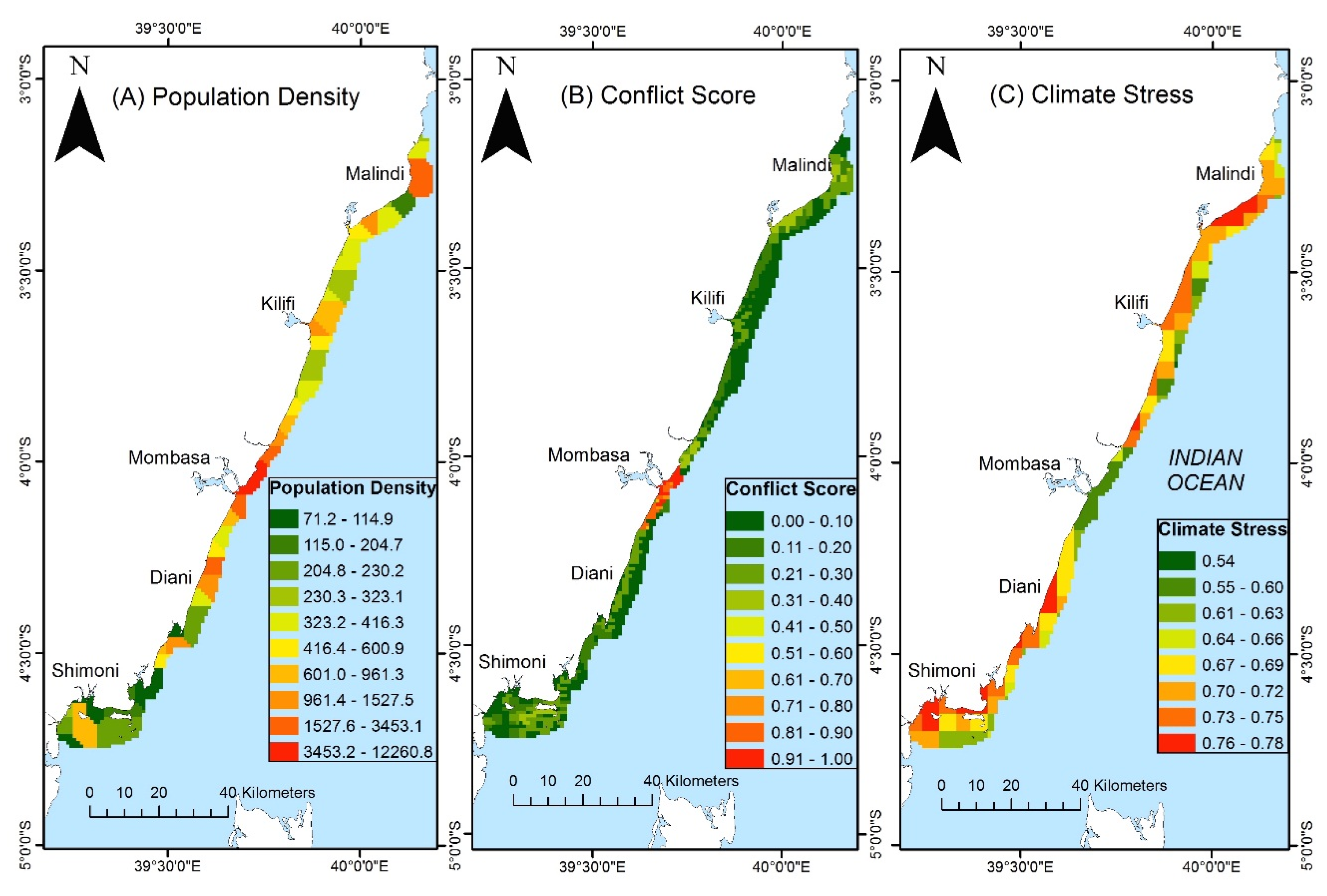
2.4. Mapping Potential Resource Use Conflicts

Potential for marine resource use conflicts was evaluated using a Spatial Multicriteria Decision Analysis and the Analytical Hierarchy Process (AHP) [34,35] following the methodology described in [24]. Briefly, the analysis of potential conflicts involved mapping of current and proposed activities, which are considered incompatible with conservation goals. These included both the existing (i.e., subsistence fishing, tourism, and waste disposal) and planned activities (i.e., sand mining, dumping and oil and gas exploration) (Tables S1 and S2). Because the activities are expected to vary in their level of incompatibility with conservation goals, we assigned relative weights to reflect the degree of incompatibility with conservation goals using the Analytical Hierarchy Process (AHP) [24]. AHP uses numerical pair-wise comparison of the relative importance of one activity over another [34,35]. Comparing the activities was achieved by asking MPA managers: which of two coastal area activities A1 and Ag is less compatible with conservation? Therefore a pair wise comparison of g activities (A1, A2, …, Ag) to reflect the importance α1, α2, …, αg of each activity in influencing overall conflict, involved constructing a g by g matrix of A which shows the dominance of the activity on the left hand side column with respect to each activity in the top row of a matrix. Decision on the relative importance of activity A1 with respect to Ag given by the entry α1g, was determined by using a nine-point intensity scale (Tables S1 and S2). The actual computation of weights involved extraction of the eigenvalues and eigenvectors from the matrix A. The normalized eigenvalues associated with the eigenvectors are the required weights α1 and αg for activities A1 and Ag respectively. Each activity map layer was created as 1-0 (Boolean) raster files, where 1 represents activity presence and 0 no activity. The weights were then aggregated and synthesized to generate a map of potential conflicts with values ranging from 0 (low potential) to 1 (highest potenti al) (See [24] for a detailed methods on mapping of potential conflicts).

2.5. Mapping Conservation Priorities

To conduct spatial prioritization analysis, we divided the study area into a regular grid of 1 × 1 km planning units (n = 1661). We classified each planning unit as either: (i) “high compliance closure”; (ii) “low compliance and recent closure”; (iii) “most destructive gear restricted”; or (iv) “no gear restricted” based on maps showing the location of protected areas, and expert knowledge on the age of protection, fishing pressure, and existing gear restrictions, (Figure 1).
Figure 1. Map of the distribution of the four fisheries management categories in place along the Kenyan coast.
Remotesensing 07 15849 g001
We used the Marxan with Probability [36] spatial prioritization tool to identify spatial priorities for a marine reserve network, while meeting a minimum representation level for all habitat types identified in the habitat maps (Table S4). Marxan with Probability uses a simulated annealing algorithm to identify a set of planning units that fulfill pre-determined quantitative targets for biodiversity features, while minimizing costs, and a probability-based cost from the likelihood of a disturbance emanating from a threat such as climate [36]. Our analyses allowed selection within all possible planning units regardless of the existing fisheries management status associated with the planning units.
We set a prioritization target for each habitat type as equal to the amount contained in existing MPAs (i.e., “high compliance closures”). We then conducted three prioritization analyses using three cost layers corresponding to three different objectives. The first sought to minimize the lost fishing opportunity by prioritizing units close to low human population because human population density and fishing effort were assumed to be positively associated [37]. The population density value of the closest land pixel from population data was allocated to the marine planning unit [38]. The second analysis identified priority areas for redistributing fishing effort away from the currently heavily fished areas using the inverse of the above cost layer. Using the inverse of human population density gives high-density areas a low cost, and thus these areas are more likely to be selected, meaning that they are protected from fishing and fishing effort will be redistributed into new areas. The third cost layer was a measure of potential resource use conflicts based on the distribution of the existing (i.e., subsistence fisheries, tourism, sand mining and dumping of dredge spoils, sewage pollution) and planned (i.e., oil and gas exploration) coastal area resource use. Prioritization sought to minimize potential conflicts that may arise from the diversified and intensified use of the inshore waters [24,39]. For each of the three costs, we formulated a planning constraint that aimed to minimize the probability of failure by prioritizing areas least exposed to climate threats. Considering the on-going debate on whether it is more effective to protect areas at greatest risk of being impacted by climate change or those that are at lowest risk [20], we explored both options. Information on climate threat exposure was taken from the existing coral reefs exposure model [29].

3. Results

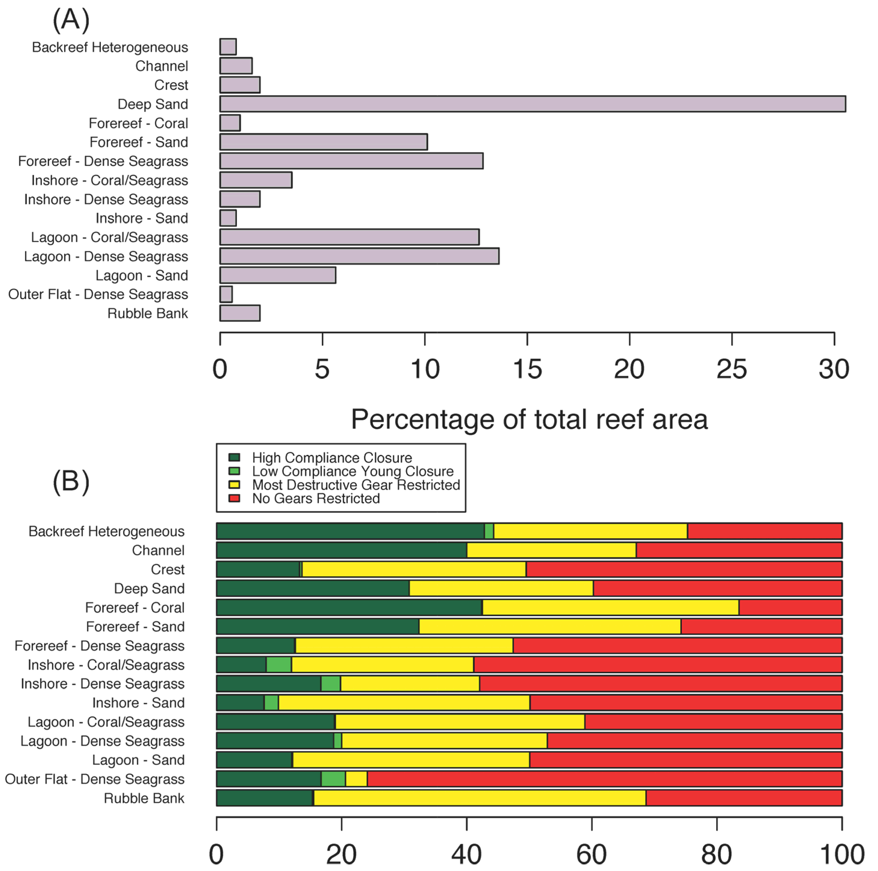
3.1. Current State of the Nearshore Habitats

The fisheries management schemes differed in their marine areal coverage, with “high compliance closures”, “low compliance and recent closures”, “all destructive gear restricted” and “no gear restricted”, covering 210, 9, 611 and 831 planning units representing 133 km2, 4.3 km2, 251 km2, and 298 km2 of habitats (all types) respectively (Figure 1). The most prevalent habitat types were deep sand, seagrass, and coral/seagrass assemblages, covering 30.5%, 29% and 17% of 686 km2 of the nearshore fringing reef area, respectively (Figure 2A). “Lagoon” was the most prominent geomorphological formations, covering 31% of the reef area (Figure 2A).
Evaluating the percentage habitats per total reef area in each management type found high representation of all habitat types in areas with no or few fisheries restrictions, i.e., “no-gear restricted” and in “most destructive gear restricted” areas (Figure 2B). However, forereef coral habitats were dominant in the “high compliance closures” and in the “most destructive gear restricted” areas. All habitat types had >10% of their total area contained within fishery closures, with some having >20% (Figure 2 and Figure 3). We found that 33% of the habitats in “high compliance closures” were coral and seagrass (covering ~77 km2), whereas higher percentages were found in the “most destructive gear restricted” and in “no-gear restricted” areas, 47% and 52% respectively (Table S3). The “low compliance and recent closure” areas contained >87% “living” category of habitat types (i.e., corals and seagrass).
Figure 2. Habitat types across four fisheries management categories (A) as a proportion of total fringing reef area; (B) as a proportion within each of the four fisheries management categories; and (C) grouped into three broad habitat groups.
Remotesensing 07 15849 g002aRemotesensing 07 15849 g002b
Figure 3. Map of habitat classification along Kenyan coast with selected areas highlighted to illustrate details.
Remotesensing 07 15849 g003

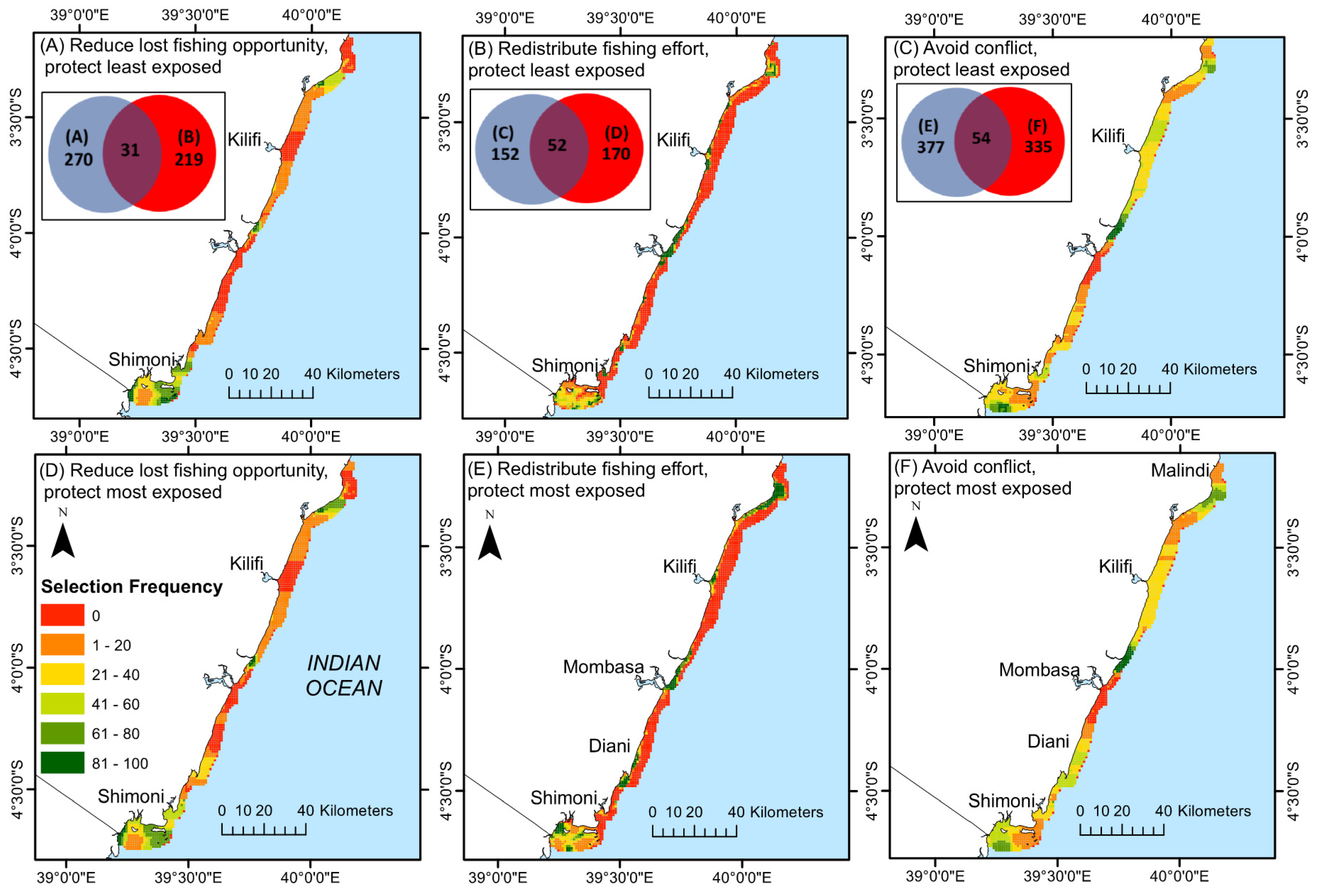
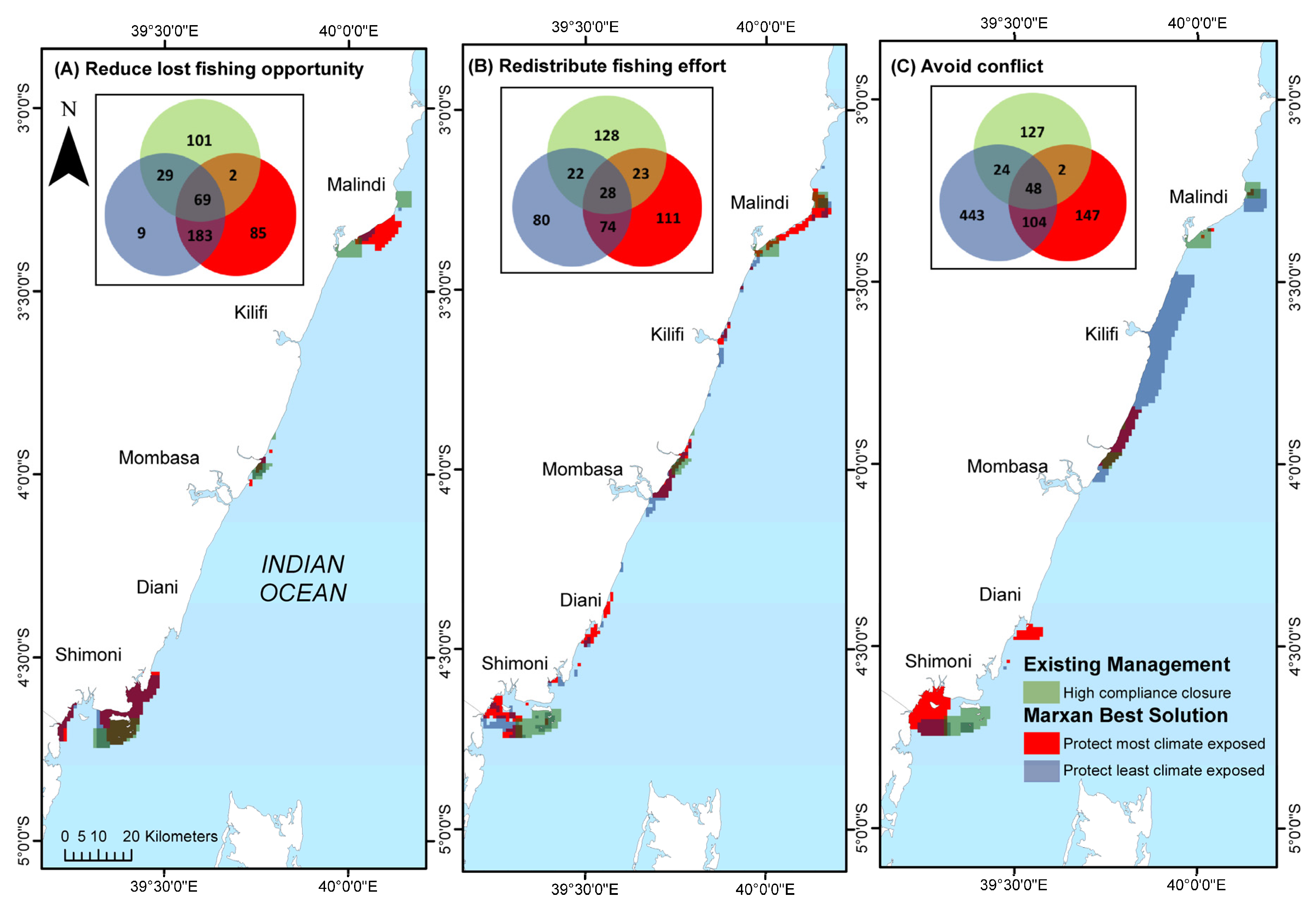
3.2. Mapping Conservation Priorities

Prioritization solutions differed considerably based on the planning objective, and on whether the analyses aimed to protect most or least exposed to climate stress. When prioritizing to minimize lost fishing opportunity and climate exposure, priority areas were concentrated just off Malindi, and north of Mombasa, thus between the “high compliance” and the “low compliance and recent” closures (Figure 4 and Figure 5A). The distribution of the priority areas constrained by the current habitat area in high compliance closures was similar when we aimed to protect areas most exposed to climate, although priorities were even more concentrated around Malindi. A smaller area (250 km2 planning units) was selected when prioritizing protected areas to minimize lost fishing opportunity and protect the most climate exposed areas compared to 301 km2 when prioritizing to protect the least climate exposed (Figure 5A,B).
When aiming to redistribute fishing efforts while protecting low climate exposure areas, clusters of priorities were more evenly distributed along the coastline, and heavily concentrated around Mombasa and north of Mombasa, around Kilifi and in the southern Kenya near the Tanzania border (Figure 5B). These priorities shifted when the aim was to protect high climate exposure areas, with priorities more heavily concentrated around Malindi (Figure 5E). Finally, when aiming to avoid potential multiple-use conflicts, results were similar regardless of whether we aimed to minimize or maximize climate exposure, with priority protected areas concentrated north of Mombasa and in the southern Kenya near Shimoni (Figure 5C,F). There were also fewer extremely low priority areas (i.e., with low selection frequency) when compared to the other cost scenarios, with most areas displaying moderate selection frequency (Figure 5C,F).
Figure 4. Map of (A) estimated relative population density pressure on marine pixels based on the population of the nearest land pixel; (B) calculated estimates of potential for resource use conflicts; and (C) coral reef climate exposure index based on the multivariate stress model.
Remotesensing 07 15849 g004
In all three prioritization scenarios, we found high priority areas to be located on the southern Kenyan coast, near the border with Tanzania and around Malindi in the north (Figure 5 and Figure 6). Scenarios for redistributing fisher effort, and avoiding conflicts also selected Diani in the south and Kilifi in the north as priority protected areas (Figure 6B,C). The total area that was constantly selected as priorities for protection (i.e., selection frequency >80%) while meeting the set target (i.e., current habitat area in high compliance closures) differed based on the planning scenarios. After redistributing fishing effort to reduce high impacts (scenario 2) and minimizing climate exposure, a smaller area was selected (i.e., 204 km2), which still meets the habitat area targets compared to the existing high compliance closures (i.e., 219 km2) (Figure 5B). Conversely, all other scenarios required similar or significantly more area than the existing closures (Figure 5). For example, prioritizing to minimize both potential multi user conflict and climate exposure required 431 km2, almost twice the area of existing high compliance closures (Figure 5C). Comparing solutions from protecting the least or the most climate-exposed revealed overlapping areas. The area selected under both climate exposure options ranged from 31 km2 when aiming to minimize lost fishing opportunity cost, to 54 km2 when aiming to avoid conflict (Figure 5). When comparing the overlap or common areas selected in different planning scenarios (e.g., redistribute fishing vs. avoid potential multi user conflict), common planning units covered a much smaller area ranging from 8–21 km2, regardless of whether the analyses minimized or maximized the climate exposure.
Figure 5. Area selection frequency (of 100 Marxan runs) based on prioritization analysis when (left) reducing the cost of lost fishing opportunity (middle) redistributing fishing effort to minimize impacts and (right) avoiding potential conflicts between ocean based activities (e.g., tourism, fishing, sand mining, oil exploration) and conservation. Figures in the first row (A,B,C) are based on protecting areas least exposed to climate change, while the second row figures (D,E,F) are based on protecting most exposed areas. Inset plots show the total area of the planning units (km2) with selection frequency >80% for each planning objective as labeled, with overlapping sections representing the area where selection frequency was >80% in both scenarios aiming to minimize environmental exposure and in scenarios aiming to maximize environmental exposure.
Remotesensing 07 15849 g005
Using the single most cost-efficient Marxan solution (Figure 6), as opposed to the areas with high selection frequency (Figure 5), shows that there is reasonable overlap between both climate exposure options, and between our identified conservation priorities and the existing high compliance closures. When aiming to minimize lost fishing opportunity cost, there is a common area of 183 km2 between the most efficient solutions for the scenario aiming to protect the least exposed and the scenario aiming to protect the most exposed to climate (Figure 6A). This level of overlap is lower, but still relatively high in the other cost scenarios (Figure 6B,C). Depending on the prioritization scenario used (i.e., minimize lost fishing opportunity, redistribute fishing effort, minimize potential for multi use conflicts), there was some overlap between both climate scenarios and existing high compliance closures. The highest overlap was under the scenario for minimizing lost fishing opportunity (69 km2, Figure 6), while the lowest was under the scenario for redistributing fishing effort 28 km2). These locations of high consensus among the three models (i.e., existing protected areas, protect the most exposed, protect the least exposed) were found within all the existing MPA’s (Kisite MPA in Shimoni, Mombasa, and in Malindi-Watamu MNP).
Figure 6. Conservation areas selected in the most cost-efficient scenario of 100 Marxan runs, based on prioritization analysis when (A) reducing the cost of lost fishing opportunity (B) redistributing fishing effort to minimize impacts and (C) avoiding potential conflicts between ocean based activities and conservation. Blue color represents priority areas when aiming to protect areas least exposed to climate change while red represents priorities when aiming to protect areas most exposed to climate change. Existing high compliance closures are shown in green. Inset venn plots show the area (number of planning units) selected under each objective, with overlapping sections representing areas which are existing high compliance closures, and which were identified as priorities when attempting to protect either the most or least exposed areas to climate change (e.g., the center of the venn plot shows the area of sites which were identified under both climate change exposure scenarios and which are existing high compliance closures).
Remotesensing 07 15849 g006

4. Discussion

4.1. Current Status of Kenyan Fringing Reef Habitats

Remote sensing spectral analyses found that Kenyan shallow reefs were dominated by lagoon geomorphological formation, with sand, seagrass, and coral assemblages as the most prevalent habitats. Coral and seagrass habitats covered 33% of the existing “high compliance closures”, while in “most destructive gear restricted” and “no-gear restricted” areas, they represented 47% and 52%. Overall, all habitat types had >10% of their total area contained within fishery closures, with some having >20%. There was high representation of all habitat types in areas with no or few fisheries restrictions (i.e., “no-gear restricted” and in “most destructive gear restricted” areas). For instance the largest proportion of living habitats (i.e., coral and seagrass) was found in areas with no or low fishing restrictions (i.e., “most destructive gear restricted” and in “no gear restricted” areas), which comprised more than twice the amount of living habitats contained within fishery closures. However, when considering habitat coverage per unit area, one third of habitat cover in the existing fishery closures was coral and seagrass. Consequently, the current configuration of managed areas protects >10% of the living categories and therefore achieves the global biodiversity targets [40]. However, when considering the high amount of coral and seagrass habitats contained in unprotected areas, and the human and climate change threats they are exposed to, the current arrangement of MPAs needs to encompass larger areas, in order to adequately protect the “living” habitats. Future studies will need to examine the other considerations and limitations particularly social considerations, as the planning process develops.

4.2. Selecting Priority Management Areas

Optimized solutions for representative habitat selection varied based on the prioritization scenario, and on whether the analysis aimed to protect the least or the most exposed to climate stress. Comparison between the three prioritization scenario solutions indicate consensus priority areas in the southern most reefs near the Kenyan-Tanzanian border, North of Mombasa and in Malindi, which are also areas where the nationally managed MPAs have existed for over ~20 years. While there was overlap between selected priority areas and the existing management areas, only 22% of the frequently selected planning priority areas coincided with the currently managed “high compliance closures”. When taking only the most cost-efficient solution from Marxan this overlap area is higher, however it is important to recognize that Marxan does not identify a perfect but instead identifies many cost-effective solutions, so using the output of a single solution may be misleading [28].
Considering the three planning scenarios, the low percentage overlap with the existing MPAs suggests that the current representation of all habitats is not ideal (i.e., Mombasa and Malindi-Watamu). Overall, our scenarios prioritized similar geographical regions as the existing MPAs (i.e., southern Kenya, around Mombasa, and Malindi-Watamu area in the north). However, the distribution of priorities within these regions differed considerably in size and location. For example, relatively larger areas were selected in southern Kenya under the scenario of minimizing lost fishing opportunity, and around Malindi when aiming to redistribute fishing effort while protecting the most exposed reefs. Interestingly, protecting most climate-exposed areas under both redistributing fisher and avoiding conflicts scenarios also prioritized Diani in southern Kenya. This area was designated as a marine reserve but insufficient consultation and stakeholder collaboration led to no implementation [41,42]. It was, however, followed up with a collaborative management system that produced the gear restrictions that were in place at the time of this spatial area designation [41]. This is an example of how planning that does not consider social considerations can lead to spatial planning failures.
Our analyses configured Marxan optimization algorithm to maximize habitats representation, all habitats being considered equally. However, it should be appreciated that habitats differ in their importance for biodiversity and fisheries production. Accessibility, resource abundance and oceanic exposure will result in some habitats being targeted more than others by specific fisheries [43]. Large swaths of rubble and sand are relatively unproductive and have lower fisheries values than seagrass and coral habitats that contain the complexity and refuge that promote high fish abundance. The optimization algorithm used here results in the selection of fewer and spatially localized areas in all the three scenarios because it did not constrain preferences to specific habitats with, for example, high biological diversity (Figure 5). Fine-scale thematic resolution mapping studies have shown that having many habitat classes and representation increases the total area required to achieve objectives, which makes it more difficult to optimize conservation designs [43]. Nevertheless, by maintaining >10% representation of coral and seagrass habitat classes in our algorithm, we show that the existing MPAs (i.e., high compliance closures) meet the suggested global biodiversity conservation goals of 10%–30% of important habitats protection [40]. Several studies have also shown that the high compliance closures have largely been effective in the recovery of fish biomass [44,45]. The success is partly attributed to considerable investment on stake-holder engagement and active enforcement through patrols, which has been necessary for addressing non-compliance issues that stem from resource use conflicts and the negative perceptions of fisheries closures [46].

4.3. Comparing Selection Scenarios

Marine spatial plans are often evaluated by their efficiency in meeting proposed conservation goals while minimizing the economic impacts [22]. Under the fisheries redistribution scenario, a smaller area is required to represent the habitat values currently in “high compliance closure” areas (i.e., meet the habitat representation goal), compared to area required under the scenarios for minimizing lost fishing grounds and for minimizing potential multi use conflicts. The area lost to fishing is highest when aiming to minimize the potential multi use conflicts, given the assumptions of no spillover and that strict protection eliminates fishing in protected areas [22]. This is true for both areas selected most frequently (Figure 5), and for the priorities identified in the single most efficient solution (Figure 6). When considering climate exposure under scenarios of minimizing lost fishing opportunity and potential conflicts, larger areas were selected when the aim was to protect the least rather than most exposed areas, which suggests a high climate exposure overall. The one exception was the large area required for redistributing fisheries while protecting the most exposed, which could be as a result of this scenario compensating for avoiding Mombasa—a high potential for resource-use conflict that contains a high concentration of diverse habitats.
Overlap of the solutions for three different planning scenarios was relatively low, with the highest being the overlap (21 km2) between redistribution of fishing effort and minimizing multiple-use conflicts while minimizing climate exposure. When comparing the single most cost-effective solution this overlap was higher, but still relatively low. Areas adjacent to highly populated areas were avoided by both scenarios because of the many uses and demand for fish near urban areas [47,48]. Minimizing conflicts resulted in the largest area (~29 km2) of the 133 km2 of the existing high compliance closures being selected at a high frequency, perhaps indicating a successful resource allocation decision in the current management system. Prioritization solutions from the fishing effort redistribution scenario appeared to redistribute areas more evenly compared to the more clustered solutions of the other two scenarios. Therefore, from the coral-reef fisheries management point of view, the fishery redistribution scenario would appear to be the ideal solution, as it represented a larger portfolio of the least and most climate-exposed areas, while at the same time being the most cost-effective solution in terms of the lost fishing grounds. Under this prioritization scenario, clusters of priorities were more evenly distributed along the coastline, with priority areas being selected within the existing protected areas and in new locations. New locations that were selected include southern Kenya between Shimoni and Diani, around Diani, south of Mombasa and around Kilifi and South of Watamu in the North.

4.4. Caveats

Despite the novelty of this study, it was not without challenges and limitations and we identify six caveats. First, the time lag between the image overpass and ground-truthing data collection can be up to two years. This can result in a mismatch between field observations and image classification and subsequent scenario modeling. We suspect, however, that many of these habitats are stable on this time scale [49]. Second, we lack a formal accuracy assessment of the habitat maps. Indeed, we lacked resources to re-survey the entire Kenya coastline for an independent accuracy assessment, and the training stage was already a big task. We reached an overall accuracy of 62% when using the training ground-truth data collection. This is a low value, furthermore theoretically optimistically biased because training quadrats were also used for accuracy assessment. Nevertheless, because of (i) the low complexity of the habitat typologies considered; (ii) classification stratified by geomorphological zones; and (iii) the density of ground-truth data, we believe the overall accuracy of the maps is above 75%, and is comparable with studies that have used similar methods with a rigorous accuracy assessment surveys [50]. Indeed, the low accuracy (62%) is partly due to the scale mismatch between the size of the quadrats (1 m2), and the class definition that matches the minimum size of mapped polygons. This scale problem in accuracy assessment protocol has been identified and discussed in [1,6]. Here, for instance the “seagrass” class includes many small patches of “sand”, that appear as “sand” in the quadrat data, hence reducing the accuracy. The 62% accuracy is thus negatively biased and conservative. Further, the low accuracy of the class “sand” is attributable to similar problems (Table S5), despite the “sand” class being the typically most accurately classified class in habitat mapping [6,8,33,50].
Third, there are multiple potential causes of coastal use conflicts, which may include resource scarcity, social power imbalances and lack of clear institutional arrangements including property rights. Yet, in this study conflict was simplified as incompatibilities between activities that may not accurately reflect the true nature of present and potential conflicts [51,52]. Fourth, we did not undertake a sensitivity analysis for the planning unit sizes, which can influence the potential to achieve habitat conservation objectives [53]. In general, we used small planning units that produced more exact habitat representation maps and expected not to over-estimate the area estimates of scenario objectives. Changing the planning unit size is expected to change the spatial patterns somewhat but the current dimensions are probably sufficient given the limited ability to implement fine-scale management. Fifth, the mapping of potential multi-user conflict is based on the existing uses (e.g., subsistence fisheries) and on future anticipated uses (e.g., sand mining, oil and gas) that have not been implemented. Changes in resource findings and government policy are likely to shift future use plans and conflict locations. Therefore, effective priority plans will need to change and be adaptive as resources and policies adapt to multiple usages. Finally, we did not consider many factors concerning the feasibility of implementing MPA’s in the priority locations we identified. When identifying conservation priorities it is important to consider the uncertainty in management outcomes and recognize that not all management actions are feasible in all locations. For example, we did not consider the cost of patrolling areas for MPA compliance, which could vary significantly based on available facilities and the level of development along the coastline.

5. Conclusions

This study demonstrated the use of very high-resolution space borne data in producing large-scale coral reef habitat maps and subsequently how these maps can support spatial prioritization decisions on the management of small-scale coral reefs fisheries. Our study analyzed multispectral imagery covering ~686 km2 of reefs along the Kenyan coast, representing one of the few national-scale, consistently processed, and very high-resolution remote sensing benthic habitat mapping applications. We then combined habitat map data with information on the existing and planned multi-stakeholder use of coastal marine areas, population density, existing fishery managed areas, and climate change related threats to identify and prioritize areas that either minimize lost fishing opportunity, redistribute fisheries away from currently heavily fished areas, or prevent potential resource use conflicts. Despite the existing Kenyan network’s apparent success in maintaining a significant proportion of “living” habitats (coral and seagrass), which are associated with higher biodiversity that underpins the small-scale fisheries [7,54], our results suggest the need for rezoning in order to establish MPA’s that are representative, anticipatory to climate change and to the current and future uses, and that are effective in enhancing fish biomass recovery.
Integrating habitat maps generated from remotely sensed data into decision support systems is expected to produce more informed and efficient planning as it more fully considers the habitats, ecosystem services, and human usages. The methodology described here combined information derived from field observations, satellites, social considerations and models used to support fisheries management decisions. Kenyan managers now have a portfolio of options that uses a robust core subset of planning units that identified a variety of realistic scenarios depending on their management constraints. The study also identifies areas for future management focus including a number of high diversity coral and seagrass habitats outside MPA.
These management options can now be explored along with other social-ecological considerations, and planning scenarios. We believe this first study combined with future iterations and more factors will allow managers to explore the full set of management options in a time-efficient manner.

Supplementary Files

Supplementary File 1

Acknowledgments

The Western Indian Ocean Marine Science Association Marine Science for Management Program (WIOMSA-MASMA) supported the procurement of the satellite imagery. The Wildlife Conservation Society through grants from the John D. and Catherine T. MacArthur Foundation supported the mapping and data analyses aspects of this study. This research was conducted with support from the Australian Research Council Centre of Excellence for Environmental Decisions. JEMW were also supported by a Discovery Grant from the Australian Research Council (DP140100733). We thank Nyawira Muthiga, James Mariara and Joan Kawaka of WCS, and Pascal Thoya and Jelvas Mwaura of KMFRI for their help with field data collection and logistics. This is an ENTROPIE contribution #79.

Author Contributions

All authors wrote the manuscript. J.M.M., K.R.J. and S.A. analyzed the data.

Conflicts of Interest

The authors declare no conflict of interest.

References

  1. Capolsini, P.; Andréfouët, S.; Rion, C.; Payri, C. A comparison of Landsat ETM+, SPOT HRV, IKONOS, ASTER, and airborne master data for coral reef habitat mapping in South Pacific Islands. Can. J. Remote Sens. 2003, 29, 187–200. [Google Scholar] [CrossRef]
  2. Walker, B.K.; Riegl, B.; Dodge, R.E. Mapping coral reef habitats in Southeast Florida using a combined technique approach. J. Coast. Res. 2008, 24, 1138–1150. [Google Scholar] [CrossRef]
  3. Andréfouët, S.; Muller-Karger, F.; Robinson, J.; Kranenburg, C.; Torres-Pulliza, D.; Spraggins, S.; Murch, B. Global assessment of modern coral reef extent and diversity for regional science and management applications: A view from space. In Proceedings of 10th International Coral Reef Symposium, Okinawa, Japan, 28 June–2 July 2004.
  4. Bruckner, A.; Rowlands, G.; Riegl, B.; Purkis, S.J.; Williams, A.; Renaud, P. Khaled bin Sultan Living Oceans Foundation Atlas of Saudi Arabian Red Sea Marine Habitats; Panoramic Press: Phoenix, AZ, USA, 2012. [Google Scholar]
  5. Rowlands, G.; Purkis, S.; Riegl, B.; Metsamaa, L.; Bruckner, A.; Renaud, P. Satellite imaging coral reef resilience at regional scale. A case-study from Saudi Arabia. Mar. Pollut. Bull. 2012, 64, 1222–1237. [Google Scholar] [CrossRef] [PubMed]
  6. Andréfouët, S. Coral reef habitat mapping using remote sensing: A user vs. producer perspective. Implications for research, management and capacity building. J. Spat. Sci. 2008, 53, 113–129. [Google Scholar] [CrossRef]
  7. Dalleau, M.; Andréfouët, S.; Wabnitz, C.C.; Payri, C.; Wantiez, L.; Pichon, M.; Friedman, K.; Vigliola, L.; Benzoni, F. Use of habitats as surrogates of biodiversity for efficient coral reef conservation planning in Pacific Ocean islands. Conserv. Biol. 2010, 24, 541–552. [Google Scholar] [CrossRef] [PubMed]
  8. Wabnitz, C.C.; Andréfouët, S.; Torres-Pulliza, D.; Müller-Karger, F.E.; Kramer, P.A. Regional-scale seagrass habitat mapping in the wider caribbean region using landsat sensors: Applications to conservation and ecology. Remote Sens. Environ. 2008, 112, 3455–3467. [Google Scholar] [CrossRef]
  9. Wilkinson, C. Status of Coral Reefs of the World: 2008; Global Coral Reef Monitoring Network and Reef and Rainforest Research Centre: Townsville, QLD, Australia, 2008; p. 296. [Google Scholar]
  10. Cinner, J.E.; McClanahan, T.R. A sea change on the African coast? Preliminary social and ecological outcomes of a governance transformation in Kenyan fisheries. Glob. Environ. Chang. 2015, 30, 133–139. [Google Scholar] [CrossRef]
  11. McClanahan, T.R.; Abunge, C.A. Perceptions of fishing access restrictions and the disparity of benefits among stakeholder communities and nations of South-Eastern Africa. Fish Fish. 2015. [Google Scholar] [CrossRef]
  12. Almany, G.; Connolly, S.; Heath, D.; Hogan, J.; Jones, G.; McCook, L.; Mills, M.; Pressey, R.; Williamson, D. Connectivity, biodiversity conservation and the design of marine reserve networks for coral reefs. Coral Reefs 2009, 28, 339–351. [Google Scholar] [CrossRef]
  13. McCook, L.J.; Ayling, T.; Cappo, M.; Choat, J.H.; Evans, R.D.; de Freitas, D.M.; Heupel, M.; Hughes, T.P.; Jones, G.P.; Mapstone, B. Adaptive management of the great barrier reef: A globally significant demonstration of the benefits of networks of marine reserves. Proc. Natl. Acad. Sci. USA 2010, 107, 18278–18285. [Google Scholar] [CrossRef] [PubMed]
  14. Roff, J.C.; Taylor, M.E. National frameworks for marine conservation—A hierarchical geophysical approach. Aquat. Conserv. Mar. Freshw. Ecosyst. 2000, 10, 209–223. [Google Scholar] [CrossRef]
  15. Pressey, R.L.; Watts, M.E.; Barrett, T.W. Is maximizing protection the same as minimizing loss? Efficiency and retention as alternative measures of the effectiveness of proposed reserves. Ecol. Lett. 2004, 7, 1035–1046. [Google Scholar] [CrossRef]
  16. Ward, T.; Vanderklift, M.; Nicholls, A.; Kenchington, R. Selecting marine reserves using habitats and species assemblages as surrogates for biological diversity. Ecol. Appl. 1999, 9, 691–698. [Google Scholar] [CrossRef]
  17. Ecoregion, WWF Eastern African Marine. Towards a Western Indian Ocean Dugong Conservation Strategy: The Status of Dugongs in the Western Indian Ocean Region and Priority Conservation Actions; World Wide Fund: Dar es Salaam, Tanzania, 2004. [Google Scholar]
  18. Duda, A.M. Strengthening global governance of large marine ecosystems by incorporating coastal management and marine protected areas. Environ. Dev. 2015, in press. [Google Scholar] [CrossRef]
  19. Aswani, S.; Hamilton, R.J. Integrating indigenous ecological knowledge and customary sea tenure with marine and social science for conservation of bumphead parrotfish (Bolbometopon muricatum) in the Roviana Lagoon, Solomon Islands. Environ. Conserv. 2004, 31, 69–83. [Google Scholar] [CrossRef]
  20. Game, E.T.; McDonald-Madden, E.; Puotinen, M.L.; Possingham, H.P. Should we protect the strong or the weak? Risk, resilience, and the selection of marine protected areas. Conserv. Biol. 2008, 22, 1619–1629. [Google Scholar] [CrossRef] [PubMed]
  21. McClanahan, T.; Cinner, J.; Maina, J.; Graham, N.; Daw, T.; Stead, S.; Wamukota, A.; Brown, K.; Ateweberhan, M.; Venus, V. Conservation action in a changing climate. Conserv. Lett. 2008, 1, 53–59. [Google Scholar] [CrossRef] [Green Version]
  22. Allnutt, T.F.; McClanahan, T.R.; Andréfouët, S.; Baker, M.; Lagabrielle, E.; McClennen, C.; Rakotomanjaka, A.J.; Tianarisoa, T.F.; Watson, R.; Kremen, C. Comparison of marine spatial planning methods in madagascar demonstrates value of alternative approaches. PLoS ONE 2012, 7, e28969. [Google Scholar] [CrossRef] [PubMed]
  23. Ban, N.C.; Mills, M.; Tam, J.; Hicks, C.C.; Klain, S.; Stoeckl, N.; Bottrill, M.C.; Levine, J.; Pressey, R.L.; Satterfield, T. A social-ecological approach to conservation planning: Embedding social considerations. Front. Ecol. Environ. 2013, 11, 194–202. [Google Scholar] [CrossRef] [Green Version]
  24. Tuda, A.O.; Stevens, T.F.; Rodwell, L.D. Resolving coastal conflicts using marine spatial planning. J. Environ. Manag. 2014, 133, 59–68. [Google Scholar] [CrossRef] [PubMed]
  25. West, J.M.; Salm, R.V. Resistance and resilience to coral bleaching: Implications for coral reef conservation and management. Conserv. Biol. 2003, 17, 956–967. [Google Scholar] [CrossRef]
  26. Obura, D.O. Resilience and climate change: Lessons from coral reefs and bleaching in the western Indian Ocean. Estuar. Coast. Shelf Sci. 2005, 63, 353–372. [Google Scholar] [CrossRef]
  27. Scheffer, M.; Barrett, S.; Carpenter, S.; Folke, C.; Green, A.J.; Holmgren, M.; Hughes, T.; Kosten, S.; van de Leemput, I.; Nepstad, D. Creating a safe operating space for iconic ecosystems. Science 2015, 347, 1317–1319. [Google Scholar] [CrossRef] [PubMed]
  28. Watts, M.E.; Ball, I.R.; Stewart, R.S.; Klein, C.J.; Wilson, K.; Steinback, C.; Lourival, R.; Kircher, L.; Possingham, H.P. Marxan with zones: Software for optimal conservation based land-and sea-use zoning. Environ. Model. Softw. 2009, 24, 1513–1521. [Google Scholar] [CrossRef]
  29. Maina, J.; McClanahan, T.R.; Venus, V.; Ateweberhan, M.; Madin, J. Global gradients of coral exposure to environmental stresses and implications for local management. PLoS ONE 2011, 6, e23064. [Google Scholar] [CrossRef] [PubMed]
  30. Obura, D.O. Participatory monitoring of shallow tropical marine fisheries by artisanal fishers in Diani, Kenya. Bull. Mar. Sci. 2001, 69, 777–791. [Google Scholar]
  31. Andrefouet, S.; Rilwan, Y.; Hamel, M.A. Habitat mapping for conservation planning in baa atoll, republic of maldives. Atoll Res. Bull. 2012, 590, 207–222. [Google Scholar]
  32. Phinn, S.R.; Roelfsema, C.M.; Mumby, P.J. Multi-scale, object-based image analysis for mapping geomorphic and ecological zones on coral reefs. Int. J. Remote Sens. 2012, 33, 3768–3797. [Google Scholar] [CrossRef]
  33. Lyzenga, D.R. Remote sensing of bottom reflectance and water attenuation parameters in shallow water using aircraft and landsat data. Int. J. Remote Sens. 1981, 2, 71–82. [Google Scholar] [CrossRef]
  34. Malczewski, J. GIS and Multicriteria Decision Analysis; John Wiley & Sons: New York, NY, USA, 1999. [Google Scholar]
  35. Saaty, R.W. The analytic hierarchy process—What it is and how it is used. Math. Model. 1987, 9, 161–176. [Google Scholar] [CrossRef]
  36. Game, E.T.; Watts, M.E.; Wooldridge, S.; Possingham, H.P. Planning for persistence in marine reserves: A question of catastrophic importance. Ecol. Appl. 2008, 18, 670–680. [Google Scholar] [CrossRef] [PubMed] [Green Version]
  37. Cinner, J.E.; Graham, N.A.; Huchery, C.; Macneil, M.A. Global effects of local human population density and distance to markets on the condition of coral reef fisheries. Conserv. Biol. 2013, 27, 453–458. [Google Scholar] [CrossRef] [PubMed]
  38. CIESIN, C. Gridded Population of the World Version 3 (GPWV3): Population Density Grids; Socioeconomic Data and Applications Center (SEDAC), Columbia University: Palisades, NY, USA, 2005. [Google Scholar]
  39. Symes, D.; Phillipson, J. Inshore Fisheries Management; Springer Science & Business Media: Dordrecht, The Netherlands, 2013; Volume 2. [Google Scholar]
  40. Wabnitz, C.C.; Andréfouët, S.; Muller-Karger, F.E. Measuring progress toward global marine conservation targets. Front. Ecol. Environ. 2009, 8, 124–129. [Google Scholar] [CrossRef]
  41. McClanahan, T.; Mwaguni, S.; Muthiga, N. Management of the Kenyan coast. Ocean Coast. Manag. 2005, 48, 901–931. [Google Scholar] [CrossRef]
  42. McClanahan, T.R. Is there a future for coral reef parks in poor tropical countries? Coral reefs 1999, 18, 321–325. [Google Scholar] [CrossRef]
  43. Hamel, M.A.; Andréfouët, S.; Pressey, R.L. Compromises between international habitat conservation guidelines and small-scale fisheries in Pacific Island countries. Conserv. Lett. 2013, 6, 46–57. [Google Scholar] [CrossRef]
  44. McClanahan, T.R.; Graham, N.A.; MacNeil, M.A.; Muthiga, N.A.; Cinner, J.E.; Bruggemann, J.H.; Wilson, S.K. Critical thresholds and tangible targets for ecosystem-based management of coral reef fisheries. Proc. Natl. Acad. Sci. USA 2011, 108, 17230–17233. [Google Scholar] [CrossRef] [PubMed]
  45. MacNeil, M.A.; Graham, N.A.; Cinner, J.E.; Wilson, S.K.; Williams, I.D.; Maina, J.; Newman, S.; Friedlander, A.M.; Jupiter, S.; Polunin, N.V. Recovery potential of the world’s coral reef fishes. Nature 2015, 520, 341–344. [Google Scholar] [CrossRef] [PubMed]
  46. McClanahan, T.R.; Davies, J.; Maina, J. Factors influencing resource users and managers’ perceptions towards marine protected area management in Kenya. Environ. Conserv. 2005, 32, 42–49. [Google Scholar] [CrossRef]
  47. Cinner, J.; Daw, T.; McClanahan, T.; Muthiga, N.; Abunge, C.; Hamed, S.; Mwaka, B.; Rabearisoa, A.; Wamukota, A.; Fisher, E. Transitions toward co-management: The process of marine resource management devolution in three East African countries. Glob. Environ. Chang. 2012, 22, 651–658. [Google Scholar] [CrossRef]
  48. McClanahan, T.; Abunge, C. Catch rates and income are associated with fisheries management restrictions and not an environmental disturbance, in a heavily exploited tropical fishery. Mar. Ecol. Prog. Ser. 2014, 513, 201–210. [Google Scholar] [CrossRef]
  49. McClanahan, T.R.; Graham, N.A.; Darling, E.S. Coral reefs in a crystal ball: Predicting the future from the vulnerability of corals and reef fishes to multiple stressors. Curr. Opin. Environ. Sustain. 2014, 7, 59–64. [Google Scholar] [CrossRef]
  50. Andréfouët, S.; Kramer, P.; Torres-Pulliza, D.; Joyce, K.E.; Hochberg, E.J.; Garza-Pérez, R.; Mumby, P.J.; Riegl, B.; Yamano, H.; White, W.H. Multi-site evaluation of ikonos data for classification of tropical coral reef environments. Remote Sens. Environ. 2003, 88, 128–143. [Google Scholar] [CrossRef]
  51. Masalu, D.C. Coastal and marine resource use conflicts and sustainable development in tanzania. Ocean Coast. Manag. 2000, 43, 475–494. [Google Scholar] [CrossRef]
  52. Cicin-Sain, B.; Belfiore, S. Linking marine protected areas to integrated coastal and ocean management: A review of theory and practice. Ocean Coast. Manag. 2005, 48, 847–868. [Google Scholar] [CrossRef]
  53. Van Wynsberge, S.; Andréfouët, S.; Gaertner-Mazouni, N.; Remoissenet, G. Conservation and resource management in small tropical islands: Trade-offs between planning unit size, data redundancy and data loss. Ocean Coast. Manag. 2015, 116, 37–43. [Google Scholar] [CrossRef]
  54. Knudby, A.; Jupiter, S.; Roelfsema, C.; Lyons, M.; Phinn, S. Mapping coral reef resilience indicators using field and remotely sensed data. Remote Sens. 2013, 5, 1311–1334. [Google Scholar] [CrossRef]

