Land Cover Mapping of a Tropical Region by Integrating Multi-Year Data into an Annual Time Series

Abstract

Generating annual land cover maps in the tropics based on optical data is challenging because of the large amount of invalid observations resulting from the presence of clouds and haze or high moisture content in the atmosphere. This study proposes a strategy to build an annual time series from multi-year data to fill data gaps. The approach was tested using the Moderate Resolution Imaging Spectroradiometer (MODIS) vegetation index and spectral bands as input for land cover classification of Colombia. In a second step, selected ancillary variables, such as elevation, L-band Radar, and precipitation were added to improve overall accuracy. Decision-tree classification was used for assigning eleven land cover classes using the International Geosphere-Biosphere Programme (IGBP) legend. Maps were assessed by their spatial confidence derived from the decision tree approach and conventional accuracy measures using reference data and statistics based on the error matrix. The multi-year data integration approach drastically decreased the area covered by invalid pixels. Overall accuracy of land cover maps significantly increased from 58.36% using only optical time series of 2011 filtered for low quality observations, to 68.79% when using data for 2011 ± 2 years. Adding elevation to the feature set resulted in 70.50% accuracy.

1. Introduction

Land use/land cover maps are important to determine vegetation distribution and to understand the variables promoting land cover change. The spatial distribution of vegetation has important implications on food security, trade, and environmental issues, like habitat loss and fragmentation. Land cover is also a key input variable to several models, for example, energy balance at the surface-atmosphere interface, hydrological cycle, and emissions of greenhouse gases. Key variables in biomass burning emission estimates are fuel load and emission factors, both highly dependent on land cover [1].

Despite its importance, recent land cover maps at a national scale in Colombia, the area of interest in this study, are scarce. The best effort has been done by the Institute of Hydrology, Meteorology, and Environmental Studies (Instituto de Hidrología, Meteorología y Estudios Ambientales, IDEAM) [2] following the Coordination of Information on the Environment (CORINE) land cover protocol, which requires multiple interpreters to update the geometry of polygons based on existing land cover maps and satellite images from 2003 to 2007. Other land cover maps for Colombia are available at the continental scale for South America [3,4,5], Latin America and the Caribbean [6,7], and the globe [8,9,10,11,12] (Table 1).

Table 1. Global and continental land cover maps for Colombia derived from satellite data.

Study Name	Sensor	Resolution (m)	Year	Source
South America (Eva et al.)	SPOT-VGT 7	1000	1995–2000	[3]
South America (Giri et al.)	Landsat	30	2010	[4]
South America (Hojas et al.)	Mainly MERIS 8	300	2008, 2010	[5]
SERENA 1	MODIS 4	500	2008	[6]
Municipalities in LAC 2	MODIS	250	2001–2010	[7]
GLOBCOVER	MERIS	300	2004–2006	[8]
GLC 2000 3	SPOT VGT	1000	2000	[9]
MODIS 4 GLC C5 5	MODIS	500	2001–2012 (annual)	[10]
Global Land Cover 1 km	AVHRR 9	1000	1992–1993	[11]
FROM-GLC 6	Landsat	30	>2006	[12]

¹ SERENA: Latin American Network for Monitoring and Studying of Natural Resources (Red Latinoamericana de Seguimiento y Estudio de los Recursos Naturales); ² LAC: Latin America and the Caribbean; ³ GLC 2000: Global Land Cover for the year 2000; ⁴ MODIS: Moderate Resolution Imaging Spectroradiometer; ⁵ MODIS GLC C5: MODIS Global Land Cover type product Collection 5; ⁶ FROM-GLC: Fine Resolution Observation and Monitoring of Global Land Cover; ⁷ SPOT-VGT: Satellite Pour l'Observation de la Terre—Vegetation program; ⁸ MERIS: Medium Resolution Imaging Spectrometer; ⁹ AVHRR: Advanced Very High Resolution Radiometer.

Table 1. Global and continental land cover maps for Colombia derived from satellite data.

Study Name	Sensor	Resolution (m)	Year	Source
South America (Eva et al.)	SPOT-VGT 7	1000	1995–2000	[3]
South America (Giri et al.)	Landsat	30	2010	[4]
South America (Hojas et al.)	Mainly MERIS 8	300	2008, 2010	[5]
SERENA 1	MODIS 4	500	2008	[6]
Municipalities in LAC 2	MODIS	250	2001–2010	[7]
GLOBCOVER	MERIS	300	2004–2006	[8]
GLC 2000 3	SPOT VGT	1000	2000	[9]
MODIS 4 GLC C5 5	MODIS	500	2001–2012 (annual)	[10]
Global Land Cover 1 km	AVHRR 9	1000	1992–1993	[11]
FROM-GLC 6	Landsat	30	>2006	[12]

¹ SERENA: Latin American Network for Monitoring and Studying of Natural Resources (Red Latinoamericana de Seguimiento y Estudio de los Recursos Naturales); ² LAC: Latin America and the Caribbean; ³ GLC 2000: Global Land Cover for the year 2000; ⁴ MODIS: Moderate Resolution Imaging Spectroradiometer; ⁵ MODIS GLC C5: MODIS Global Land Cover type product Collection 5; ⁶ FROM-GLC: Fine Resolution Observation and Monitoring of Global Land Cover; ⁷ SPOT-VGT: Satellite Pour l'Observation de la Terre—Vegetation program; ⁸ MERIS: Medium Resolution Imaging Spectrometer; ⁹ AVHRR: Advanced Very High Resolution Radiometer.

The generation of land cover maps using optical data in areas with persistent clouds is challenging [13]. For instance, filtering daily Moderate Resolution Imaging Spectroradiometer (MODIS) data over Colombia for the entire year of 2008 resulted in an area of 4.1% without any valid information, mainly due to clouds along the Pacific coast and in the Andean cordilleras [6]. At tropical latitudes MODIS acquires images at least every other day. The standardized data processing chain aggregates, for instance, all acquisitions over a 16-day period to generate a vegetation index composite. Data compositing is a viable approach to reduce the effect of invalid observations, data noise, or observations with high view or sun zenith angles by rule sets or statistical functions. Nevertheless, there are regions without any valid observation for the entire compositing period, e.g., due to persistent cloud cover. In MODIS data these pixels are flagged by the quality assurance science data set and the user has the flexibility to decide which quality level is acceptable and how to deal with invalid data for a particular application. For instance, temporal interpolation of data gaps is a frequently employed technique to reconstruct a continuous time series for land cover mapping, but the length of the period of missing data impacts the accuracy [14].

A time series, in the context of remote sensing, is defined as the dense monitoring of surface dynamics over a defined period [15]. The extraction of one pixel from this sequence of images ordered in time shows the temporal behavior of the land surface which may be decomposed in three components: the trend(s), the cyclic or other seasonal behavior, and irregular fluctuations [16]. There are several computer programs to generate time series from satellite data. Harmonic Analysis for Time Series (HANTS), for instance, employs the Fast Fourier Transformation to model the general temporal behavior of a time series and iteratively substitutes invalid observations (mostly cloudy pixels in vegetation indices) defined by a threshold exceeding a negative deviation from the modeled data [17]. The Timesat software models smooth time series by mathematical functions or filters, generally applying a fitting to the highest values of vegetation index values [18,19]. The Time Series Generator (TiSeG) applies user-defined quality settings to pixel-level quality information provided with each MODIS land product and generates spatial and temporal indices of data availability and gap length [20,21]. In a second step, data gaps may be masked or interpolated using generic temporal interpolation approaches, such as linear interpolation, cubic spline, or polynomial functions. An alternative approach employs stepwise interpolation of short data gaps by iteratively decreasing the data quality [21]. There are recent studies employing time series models for land cover and land cover change mapping often employing complex time series models [22,23,24]. The common question which all approaches address is how to identify, handle, and replace invalid observations.

In the context of classification, features are needed to distinguish the different land surface properties and land cover or vegetation classes. Commonly, spectral information from multiple portions of the electromagnetic spectrum is employed to distinguish different land cover classes. The spectral characteristics of dense green vegetation, for instance, are a low reflectance in the visible wavelengths and high values in the near infrared, which are fundamentally different from water, with generally low and decreasing reflectance in the visible to mid-infrared range of the electromagnetic spectrum. This multispectral information may be complemented by temporal information. In this context, time series describe the temporal properties of land surface types and may allow distinguishing between deciduous forests, typically described by a uni-modal curve of green-up, plateau, and senescence of a vegetation index, from an evergreen forest with constantly high values. In this respect, the phenological development of natural and managed vegetation plays a major role in image classification [25,26,27,28,29]. Even though spectral and temporal properties for many land cover classes are well defined, it may be difficult to separate some classes, e.g., bare soil from urban areas. Information from the microwave range of the electromagnetic spectrum may improve separability of such classes, as the geometry of objects with strong backscattering at buildings is fundamentally different from the weak backscatter of bare soils. Information from Synthetic Aperture Radar (SAR) images may also be helpful for mapping regions of frequent cloud cover, such as Colombia, as long waves penetrate clouds and have shown potential to improve forest classifications by going well into the canopy [30]. However, classifications from radar data alone have not shown promising results due to limited spectral resolution [31,32]. The horizontal (H) or vertical (V) orientation of electromagnetic fields, known as polarimetry, has been used in order to determine differences in land cover backscattering to overcome this limitation of radar images [33,34].

The objective of this study was to generate a land cover map from satellite image time series for the national territory of Colombia, which includes regions of frequent cloud cover. The primary goal was to generate an annual time series of vegetation index and spectral data to accurately classify eleven land cover classes of Colombia. In a second step, additional variables such as radar backscatter, precipitation, and elevation were added to improve the land cover map.

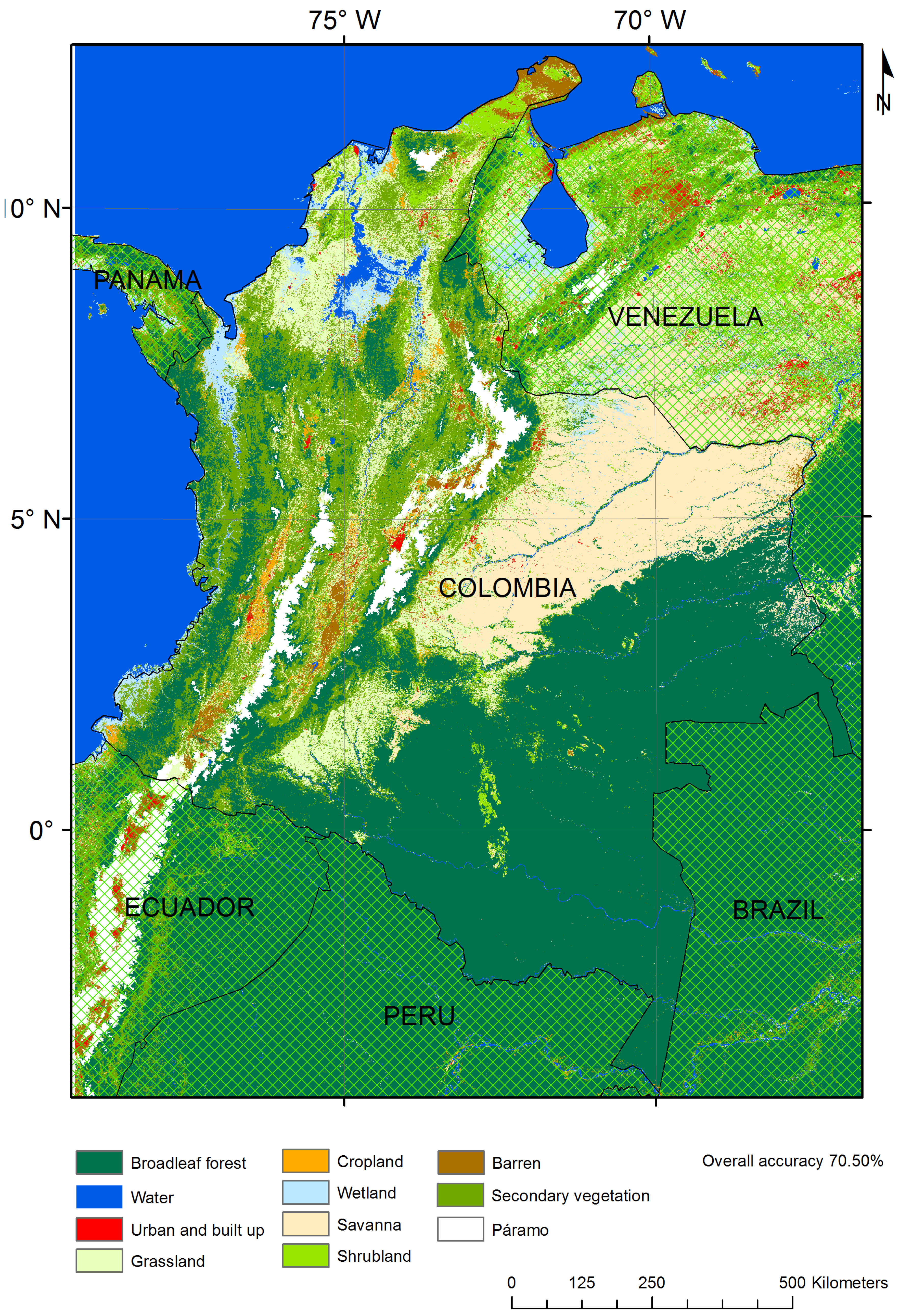
2. Data and Preprocessing

Six MODIS tiles (h10-h11/v07-v09) of the 16-day vegetation index composite product of 500 m spatial resolution (MOD13A1) were downloaded from http://reverb.echo.nasa.gov/. In addition to the Normalized Difference Vegetation Index (NDVI) four spectral bands of surface reflectance were used: blue (0.459–0.479 µm), red (0.620–0.670 µm), near-infrared (0.841–0.876 µm), and short-wave infrared (2.105–2.155 µm). The MODIS Reprojection Tool (MRT) was employed to generate mosaics (23 per year) and transformed data to the Universal Transverse Mercator (UTM) projection. Thirteen years of MOD13A1 data (January 2001–December 2013) were used to study the temporal and spatial distribution of cloud content and five years (2009–2013) were used as explanatory variables for land cover classification. In order to study improvements in accuracy, three ancillary variables were also included: Phase Array type L-band Synthetic Aperture Radar (PalSAR) HH (500 m) available for South America at www.eorc.jaxa.jp/ALOS/en; mean annual precipitation, and digital elevation model (1000 m) available at www.worldclim.org [35]. These ancillary explanatory variables were added to the annual time series of MODIS MOD13A1 data using nearest neighbor resampling to 500 m spatial resolution.

3. Study Area

The continental extension of Colombia is 1,141,748 km². The national territory is located in the neotropics, ranging from the Caribbean Sea (12° North) to the northern Amazon basin (4° South) and from the Orinoco river (67° West) to the Pacific Ocean (79° West). The country is commonly divided in five regions: Caribbean, dominated by grasslands, wetlands and bare soils; Pacific, made up of pluvial and very humid rain forest; Orinoco, dominated by savannas in a flat landscape; the rain forest area of the Amazon; and the Andes mountains, with highly modified natural ecosystems, an important crop extension, road networks, and built-up areas. Important activities promoting land use and change in Colombia are related to illegal cropping [36], mining, agriculture, and deforestation [37]. The main climate controls of this region with abrupt topography are: the Inter-tropical Convergence Zone (ITZC), the two low-level jet streams (Chocó and San Andrés), the feedback of the Amazon evapotranspiration, and the El Niño-Southern Oscillation (ENSO) [38]. The topographic effect is important since approximately one third of the country (392,380 km²) is covered by mountains. This includes Chocó-Darién moist forests, Northern Andean Montane Forests, and Santa Marta Montane Forests [39].

4. Methods

4.1. Annual Time Series Generation from Multi-Year Image Composites

TiSeG [20,21] was used to identify invalid observations and analyze data availability according to the pixel-level quality information provided with MODIS vegetation index products [40,41]. Only pixels that were flagged as good or acceptable general quality, a perfect to intermediate usefulness index, good or marginal data reliability, and no mixed clouds, snow/ice, and shadow were kept for further processing.

Figure 1 illustrates the time series generation approach by integrating multi-year data to generate an annual time series as proposed in this study. It employs hypothetical NDVI data to describe a bi-modal curve, e.g., typical for bi-seasonal dryland agriculture in inner-tropical regions. Figure 1A shows an annual time series for 2011 (Y_n), where the grey line, joining small and large circles, indicates the annual time series without data quality analysis and the black line, connecting only large circles of valid observations, the linear temporal interpolation of all valid observations. The latter resembles the common time series generation approach by inferring invalid observations from previous and posterior valid samples as implemented in most time series generation packages. Note that the longest data gap is 13 composites (the compositing length is 16 days) which corresponds to more than half-a-year. Figure 1B shows five annual time series (different colors) with circles indicating the valid observations and lines for the linear temporal interpolation. Neither time series resembles the expected bimodal temporal profile.

Multi-year data integration employs data of other years to shorten data gaps and properly represent the seasonal cycles of land surface types. It builds upon two premises: (1) a seasonal cycle with no or insignificant variability in time and magnitude between years, and (2) no change of the land cover. The basic idea is to maintain valid observations of the initial year even if there were also valid observations in the other years. Invalid pixels of the initial year are replaced by valid pixels of the same composite from other years. In case of multiple valid observations a rule needs to be applied, e.g., the mean of all valid observations. The specific step-wise implementation in this study is shown in Figure 1C,D, where the colors indicate the year to which the observation belongs (or their respective mean) with void circles and grey lines showing the annual time series of valid observations of individual years (Figure 1B) and filled circles and a black line the annual time series of integrated data. First, data of the previous and posterior year (Y_n ± 1) were analyzed, i.e., data from years 2010 and 2012 (Figure 1C). All valid observations from 2011 remain, even if there were other valid observations in 2010 or 2012 (composite 1 and 4 for 2010). Invalid observations in 2011 were replaced by valid observations of either 2010 or 2012 (composite 11 and 23 for 2010 and 2, 12, and 15 for 2012). In case of valid observations in both years, the mean was calculated (composite 3 and 6). This time series better represents the expected bi-modal temporal curve but has deficiencies in particular in the second half of the year due to the remaining long data gaps of five composites (approximately 2.5 months). A second step (Figure 1D) integrates data from 2009 and 2013 (Y_n ± 2) to the previously-generated time series of Figure 1C. Existing data were not altered regardless of their origin (2010, 2011, 2012, or the mean of 2010 and 2012) and only gaps are closed either with data from 2009 (composite 9, 13, and 16), 2013 (composite 8, 14, and 19), or their mean in case both were valid (composite 17). The resulting annual time series mimics the expected bi-modal temporal profile. There are still some data gaps (composite 5, 10, 18, and 21), but these are short and can be reasonably inferred by linear temporal interpolation or kept as missing data, depending on the application.

Figure 1. Multi-year data integration for time series generation. The hypothetical data should represent an annual time series with bi-modal characteristics, typical for agriculture with two growing seasons. (A) Time series of 2011 of valid (large circles) and invalid (small circles) observations connected by a grey line and linear temporal interpolation of valid data shown by a black line; (B) annual time series from valid observations of five years in different colors; (C) integrated time series from data of 2011 ± 1 year; and (D) integrated time series from 2011 ± 2 years, based on (C). Void circles and grey lines in (C) and (D) indicate valid data and linear interpolation of annual data from (B).

Figure 1. Multi-year data integration for time series generation. The hypothetical data should represent an annual time series with bi-modal characteristics, typical for agriculture with two growing seasons. (A) Time series of 2011 of valid (large circles) and invalid (small circles) observations connected by a grey line and linear temporal interpolation of valid data shown by a black line; (B) annual time series from valid observations of five years in different colors; (C) integrated time series from data of 2011 ± 1 year; and (D) integrated time series from 2011 ± 2 years, based on (C). Void circles and grey lines in (C) and (D) indicate valid data and linear interpolation of annual data from (B).

4.2. Reference Data for Training and Legend Definition

The International Geosphere-Biosphere Programme (IGBP) land cover legend [42] was used to classify the MODIS time series of vegetation indices and spectral bands into land cover classes. The IGBP system has 16 classes but only nine are present in Colombia: broadleaf forest, water, urban and built-up, grassland, cropland, wetland, savanna, shrubland, and barren. Two land cover classes were added to the legend given their extent and ecological importance: secondary vegetation and páramo. Secondary vegetation is important due to agricultural land use, shifting cultivation, and illegal cultivation in natural ecosystems [37,43]. Páramo, is a unique tropical high-elevation (>3000 m.a.s.l.) ecosystem ranging from Costa Rica to Peru [44]. The updated delimitation of páramo at a scale of 1:100.000 was used to define the limits of this ecosystem [45].

The training sites were sampled from the national vegetation map of IDEAM [46]. Table 2 shows the class aggregation scheme from 18 classes of IDEAM to nine classes of the IGBP legend; class “snow” was aggregated to barren since the area is too small to be considered in the training process. Training sites were only selected in core areas of the reference cartography (i.e., IDEAM map) at least 500 m away from other land cover classes (3 × 3 kernel of which all pixels had the same class as the central pixel [47]). More training data as relative to its expected area from the IDEAM map were sampled for barren, broadleaf forests and secondary vegetation to mitigate confusion with urban and built-up and shrubland [47].

Table 2. Aggregation of the national vegetation map [46] with 18 classes to nine IGBP classes and adding secondary vegetation and páramo. Training samples were derived from the national vegetation map and visual interpretation of high spatial resolution satellite images.

IGBP	Official Vegetation Map	Training Pixels
Broadleaf forest	Natural forests, Forest plantation	1459
Water	Continental water bodies, Artificial continental water bodies, Costal lagoons	730
Urban and built-up	Urban areas	461
Grassland	Grassland	652
Cropland	Permanent and semi-permanent crops, Agricultural areas, Annual and transitory crops	469
Wetland	Continental hydrophytic vegetation	528
Savanna	Savannas, Costal shrublands and savannas	982
Shrubland	Shrubland	668
Barren	Highly-modified areas, Bare soil, Glaciers and snow, Bare rock	1502
Secondary vegetation	Secondary vegetation (added to IGBP legend)	1157
Páramo	Páramo (added to IGBP legends)	681

Table 2. Aggregation of the national vegetation map [46] with 18 classes to nine IGBP classes and adding secondary vegetation and páramo. Training samples were derived from the national vegetation map and visual interpretation of high spatial resolution satellite images.

IGBP	Official Vegetation Map	Training Pixels
Broadleaf forest	Natural forests, Forest plantation	1459
Water	Continental water bodies, Artificial continental water bodies, Costal lagoons	730
Urban and built-up	Urban areas	461
Grassland	Grassland	652
Cropland	Permanent and semi-permanent crops, Agricultural areas, Annual and transitory crops	469
Wetland	Continental hydrophytic vegetation	528
Savanna	Savannas, Costal shrublands and savannas	982
Shrubland	Shrubland	668
Barren	Highly-modified areas, Bare soil, Glaciers and snow, Bare rock	1502
Secondary vegetation	Secondary vegetation (added to IGBP legend)	1157
Páramo	Páramo (added to IGBP legends)	681

4.3. Classification

A decision-tree method was used for land cover classification since it does not require the assumption of normally-distributed data and is able to handle noisy or missing observations [11]. Other important properties of tree-based modeling are that it provides information on the importance of predictive data, allows for the selection of pixels with the best confidence, and has built-in options for boosting. Boosting is a meta-strategy that combines several basic classifications in order to obtain better accuracies, as each new classifier intends to reduce the error of the previous iteration [48,49]. In addition, along with the final discrete classification decision trees provide a pixel-level confidence estimate which may be used to obtain spatial information of map quality [50,51].

C5.0 was used for decision-tree classification [52] and the built-in option of ten-folded boosting allows for obtaining a confidence estimate of each class assignment [53]. Confidence maps have been successfully used in several remote sensing studies to describe areas of higher uncertainties in class assignment, area calculation, and assessing map accuracy or performing map comparison [6,7,54]. Lower confidences are expected in case of ambiguity in class assignment, either due to an unclear description by the explanatory variable set or highly fragmented, fine-scale structures.

4.4. Validation Sample Design

The most recent version of the national land cover map was used as reference data for accuracy assessment. This official map was made following the CORINE Land Cover (CLC) image interpretation method, with a 1:100,000 scale using Landsat images [2]. The map is independent from the vegetation land cover map used for the training sample allocation as recommended by Strahler et al. [51]. The CLC legend was designed as a function of the thematic level of detail, a first level of five classes (urban and built-up, crops, forests, wetlands, and water bodies) subdivided in a second level of 15 classes and a third level of 57 classes. These 57 classes were aggregated to the 11 predefined classes. Each pixel of the CLC map was given the chance of being selected for the validation sample data through a stratified random sampling design (Table 3). The sample size for validation corresponds to 1% of the pixels stratified by land cover classes (n = 45,596), no clusters or sample units were required since reference data is available for the full extension of the study area. Misregistration is expected to be low, because Landsat, as reference data source, and MODIS, used for image classification, were found to be well co-registered (error less than one Landsat pixel) [55,56,57]. An error matrix [58], with the assessment unit being the pixel, was calculated for each variable setup in order to determine overall accuracy, the Kappa coefficient, and omission/commission errors.

All maps were compared to each other using two statistical tests. McNemar test (Equation (1)) performs pair-wise comparisons of the frequency f of correctly classified samples in map A that were incorrectly classified in map B and vice versa [59].

$$z=\frac{f_{AB}-f_{BA}}{\sqrt{f_{AB}+f_{BA}}}$$

(1)

The difference in overall accuracies (OA) was statistically tested with Equation (2) where VAR refers to the variances of the samples from map A and B.

$$z=\frac{\left|O{A}_A-O{A}_B\right|}{\sqrt{VA{R}_A+VA{R}_B}}$$

(2)

Table 3. Aggregation of CLC [2] classes into IGBP classes, 1% of the pixels were randomly selected from each class for accuracy assessment.

IGBP	CORINE Land Cover	Validation Pixels
Broadleaf forest	Agroforestry, forest plantations, tall and dense forest, open tall and dense forest, riparian vegetation, inundated forests, open inundated forests.	22,137
Water	Exposed sediments at low tides, rivers, lakes, channels, artificial water bodies, coastal lagoons, sea and ocean, aquaculture, artificial water bodies.	774
Urban and built-up	Urban, infrastructure, landfill, waste dump, urban park, recreational infrastructure, greenhouse crops.	112
Grassland	Grassland, mosaic grassland crops, forage crops, transitory crops, permanent crops, forage crops, open grassland with crops.	6281
Cropland	Transitory crops, permanent crops.	434
Wetland	Swamp, peatland, aquatic vegetation, costal swamp, high salinity water bodies, inundated savanna.	523
Savannas	Open areas without vegetation, savanna, open shrubland.	5454
Shrubland	Shrubland, open forest, grasses and shrublands, shrubland.	1060
Barren	Mining, dunes, bare rock, degraded lands, glacier or snow, beaches, dunes.	272
Secondary vegetation	Agricultural mosaic, fragmented forest, secondary vegetation, tall secondary vegetation, grasses and shrublands.	7239
Páramo	Added from [45]	1310

Table 3. Aggregation of CLC [2] classes into IGBP classes, 1% of the pixels were randomly selected from each class for accuracy assessment.

IGBP	CORINE Land Cover	Validation Pixels
Broadleaf forest	Agroforestry, forest plantations, tall and dense forest, open tall and dense forest, riparian vegetation, inundated forests, open inundated forests.	22,137
Water	Exposed sediments at low tides, rivers, lakes, channels, artificial water bodies, coastal lagoons, sea and ocean, aquaculture, artificial water bodies.	774
Urban and built-up	Urban, infrastructure, landfill, waste dump, urban park, recreational infrastructure, greenhouse crops.	112
Grassland	Grassland, mosaic grassland crops, forage crops, transitory crops, permanent crops, forage crops, open grassland with crops.	6281
Cropland	Transitory crops, permanent crops.	434
Wetland	Swamp, peatland, aquatic vegetation, costal swamp, high salinity water bodies, inundated savanna.	523
Savannas	Open areas without vegetation, savanna, open shrubland.	5454
Shrubland	Shrubland, open forest, grasses and shrublands, shrubland.	1060
Barren	Mining, dunes, bare rock, degraded lands, glacier or snow, beaches, dunes.	272
Secondary vegetation	Agricultural mosaic, fragmented forest, secondary vegetation, tall secondary vegetation, grasses and shrublands.	7239
Páramo	Added from [45]	1310

5. Results

5.1. Spatial and Temporal Distribution of Invalid Pixels

Climate and topography defined the spatial and temporal distribution of invalid pixels. The statistics of invalid pixels from 2001 to 2013 (n = 13) ranged from a minimum of 544,211 km² (47.7%) in 2001 to a maximum of 626,218 km² (54.9%) in 2011 (Figure 2A) with an average area of 574,457 km²(50.4%). For a single year (2011 in Figure 2B) there is a bimodal distribution of invalid pixels. This temporal pattern is valid for most parts of the country and follows the annual shifts of the low-pressure belt of the intertropical convergence zone (ITCZ) with two rainy seasons intercalated by dry and semi-dry periods.

Figure 2. Temporal distribution of invalid pixels. (A) Average of 23 16-days composites per year describing inter-annual variability of invalid data from 2001 to 2013. The inter-annual average is 50.4%; and (B) temporal distribution of invalid data in 2011 with a dry season at the beginning of the year (date 1) and at the end of the year (date 23), with two rainy seasons separated by a semi-dry season (dates 13–19). The percentage of invalid pixels ranges from a minimum of 26% (January) to a maximum of 87% (April) with an average of 54.9%.

Figure 2. Temporal distribution of invalid pixels. (A) Average of 23 16-days composites per year describing inter-annual variability of invalid data from 2001 to 2013. The inter-annual average is 50.4%; and (B) temporal distribution of invalid data in 2011 with a dry season at the beginning of the year (date 1) and at the end of the year (date 23), with two rainy seasons separated by a semi-dry season (dates 13–19). The percentage of invalid pixels ranges from a minimum of 26% (January) to a maximum of 87% (April) with an average of 54.9%.

The spatial distribution of invalid pixels is related to the cloud formation [38], by wind convergence over the Pacific Ocean and the orographic effect of the Andes (Figure 3A shows data for 2011). This map was regionalized in four categories, low, intermediate, high, and very high (see Figure 3B) defined by natural breaks (Jenks) unsupervised classification method (Table 4).

Table 4. Categorization of invalid pixels of 2011 in four classes (low, intermediate, high, very high) using thresholds according to natural breaks (Jenks) unsupervised clustering.

Invalid Pixels	Category	Area (km2)	Area (%)
0–8	Low	176,703	15.6
9–12	Intermediate	438,189	38.6
13–18	High	356,207	31.1
19–23	Very high	167,916	14.7

Table 4. Categorization of invalid pixels of 2011 in four classes (low, intermediate, high, very high) using thresholds according to natural breaks (Jenks) unsupervised clustering.

Invalid Pixels	Category	Area (km2)	Area (%)
0–8	Low	176,703	15.6
9–12	Intermediate	438,189	38.6
13–18	High	356,207	31.1
19–23	Very high	167,916	14.7

Figure 3. Spatial distribution (A) of invalid pixels for 2011 with dark areas showing high frequency (maximum 23 composites per year) and (B) depicting a categorization into four classes using natural breaks (Jenks) unsupervised clustering for data ranges (see Table 4).

Figure 3. Spatial distribution (A) of invalid pixels for 2011 with dark areas showing high frequency (maximum 23 composites per year) and (B) depicting a categorization into four classes using natural breaks (Jenks) unsupervised clustering for data ranges (see Table 4).

5.2. Multi-Year Data Integration for Time Series Generation

Multi-year data integration allows a better reconstruction of phenological patterns of vegetation classes. Figure 4 shows the effect of eliminating invalid pixels and adding data from adjacent years for two pixels representing evergreen broadleaf forest and savannas, where the color of large filled circles indicates the compositing step with data from 2011 ± 1 year and 2011 ± 2 years. In both cases time series are improved by replacing invalid values, but the use of the importance of the multi-year approach is best noted for temporal profiles with seasonal cycles due to vegetation phenology. For the evergreen broadleaf forest site in Figure 4A there is, as expected, no seasonal dynamic; thus, there are only minor modifications by multi-year data integration as compared to time series generation using data from 2011, only. For the savanna site in Figure 4B there is a moderate seasonal dynamic, responsive to low precipitation.

Invalid data was drastically reduced when using compositing with adjacent years. Both the mean and the standard deviation (shown in parenthesis) were reduced; for 2011 the mean invalid data without compositing was 54.9% (17.9%), which reduced to 25.0% (11.5%) for 2011 ± 1 year and 15.2% (6.3%) for 2011 ± 2 years. This reduction was more evident for 16-day composites with the highest proportion of invalid pixels during the rainy season (composites 6–13 and 17–23 in Figure 5A). From the spatial point of view, the reduction occurs in all categories (Figure 5B). The area of no observation for the entire year was reduced from 24,130 km² (2.11%) in 2011 to 2890 km² (0.25%) for 2011 ± 1 year and to 1497 km² (0.13%) for 2011 ± 2 years.

Figure 4. Time series with multi-year data integration using valid observations and interpolation. Large filled circles indicate data used for the time series, void circles show omitted data. (A) Evergreen broadleaf forest (2.95086° N, 69.80172° W); and (B) savanna (3.49735° N, 72.29125° W).

Figure 4. Time series with multi-year data integration using valid observations and interpolation. Large filled circles indicate data used for the time series, void circles show omitted data. (A) Evergreen broadleaf forest (2.95086° N, 69.80172° W); and (B) savanna (3.49735° N, 72.29125° W).

Figure 5. Reduction of invalid pixels by multi-year data integration for 2011, employing data ± 1 or ± 2 years. (A) Reduction of the percentage of invalid pixels over the course of the year; and (B) reduction of invalid pixels for each spatial category of invalid pixels (Figure 3B and Table 4).

Figure 5. Reduction of invalid pixels by multi-year data integration for 2011, employing data ± 1 or ± 2 years. (A) Reduction of the percentage of invalid pixels over the course of the year; and (B) reduction of invalid pixels for each spatial category of invalid pixels (Figure 3B and Table 4).

5.3. Image Classification and Assessment

Several maps were obtained based on different scenarios to handle invalid pixels and to include ancillary variables. Specifically, the following scenarios (time series, TS) were tested:

• TS: Stacking of MODIS data of 2011 without quality analysis
• TS-F: Stacking of MODIS data of 2011 and filtering for low-quality observations
• TS-F-C1: As TS-F followed by composting with valid data from ± 1 year
• TS-F-C2: As TS-F followed by composting with valid data from ± 2 years
• TS-F-I: As TS-F followed by linear temporal interpolation of data gaps
• TS-F-C1-I: As TS-F-C1 followed by linear temporal interpolation of remaining data gaps
• TS-F-C2-I: As TS-F-C2 followed by linear temporal interpolation of remaining data gaps
• -E: Adding explanatory variable elevation
• -R: Adding explanatory variable L-band Radar data
• -P: Adding explanatory variable mean annual precipitation

Two analyses were carried out to assess the quality of each map: (1) confidence-based quality assessment for invalid pixels stratified by four categories, and (2) accuracy and error calculation based on the error matrix using reference samples.

5.3.1. Confidence-Based Assessment

Map confidence was calculated for different scenarios of stacking, filtering, compositing, interpolation, and adding other variables (see the list specified above). Table 5 shows the mean confidence for each category of invalid pixels as defined by natural breaks (Jenks) using unsupervised classification (Figure 3B, Table 4). There is the expected pattern of decreasing confidence with increasing invalid data from categories low to very high. It was found that confidence decreases when invalid pixels are removed from the explanatory variables (TS-F). Using valid data from previous or posterior years increased confidences for all categories (TS-F-C1, TS-F-C2). These differences were most notable for categories with more invalid data (high and very high). Interpolation after quality analysis (TS-F-I) depicts a moderate improvement over a simple layer stack (TS). Interpolation of the remaining data gaps in multi-year time series (TS-F-C1-I, TS-F-C2-I) shows some decreases in confidence in comparison to no interpolation (TS-F-C1, TS-F-C2). Confidences marginally changed by adding additional explanatory variables (-E, -R, -P) to time series TS-F-C2.

Table 5. Confidence-based quality assessment of land cover classifications for each category based on a specific scenario to handle invalid pixels. TS: time series, F: filtering for low-quality observations, Cx: compositing with ± x years, I: linear temporal interpolation, E: elevation, R: Radar data, and P: precipitation. Grey cells mark best results for runs with and without ancillary data.

Category	TS	TS-F	TS-F-C1	TS-F-C2	TS-F-I	TS-F-C1-I	TS-F-C2-I	TS-F-C2-E	TS-F-C2-R	TS-F-C2-P
Low	0.70	0.55	0.76	0.74	0.71	0.71	0.71	0.76	0.74	0.75
Intermediate	0.70	0.55	0.78	0.76	0.73	0.72	0.72	0.79	0.76	0.77
High	0.56	0.37	0.68	0.65	0.61	0.61	0.62	0.70	0.65	0.66
Very high	0.49	0.21	0.71	0.67	0.50	0.56	0.57	0.69	0.65	0.64

Table 5. Confidence-based quality assessment of land cover classifications for each category based on a specific scenario to handle invalid pixels. TS: time series, F: filtering for low-quality observations, Cx: compositing with ± x years, I: linear temporal interpolation, E: elevation, R: Radar data, and P: precipitation. Grey cells mark best results for runs with and without ancillary data.

Category	TS	TS-F	TS-F-C1	TS-F-C2	TS-F-I	TS-F-C1-I	TS-F-C2-I	TS-F-C2-E	TS-F-C2-R	TS-F-C2-P
Low	0.70	0.55	0.76	0.74	0.71	0.71	0.71	0.76	0.74	0.75
Intermediate	0.70	0.55	0.78	0.76	0.73	0.72	0.72	0.79	0.76	0.77
High	0.56	0.37	0.68	0.65	0.61	0.61	0.62	0.70	0.65	0.66
Very high	0.49	0.21	0.71	0.67	0.50	0.56	0.57	0.69	0.65	0.64

5.3.2. Error Matrix-Based Assessment

The error matrix was used to evaluate overall accuracy, Kappa coefficient, and errors of omission and commission of land cover maps obtained under different scenarios. First, we determined the best annual time series using MODIS data from 2011 integrating data from previous and posterior years, to which we added ancillary explanatory variables in a second step to test further improvements. Pairwise tests of statistically significant differences between maps and overall accuracies were obtained with the McNemar test and standard z-test, respectively. Red (p < 1%) and orange (p < 5%) cells in Figure 6 show statistically significant differences between maps (McNemar) in the lower left (below the diagonal) and between overall accuracies in the upper right.

Figure 6. Statistical comparison among classifications using the McNemar (lower-left triangle) and overall accuracy (upper-right triangle) significance tests. Grey cells indicate no significant difference, orange indicates significant differences p < 5% and red significant differences p < 1% using a two-tailed z-test.

Figure 6. Statistical comparison among classifications using the McNemar (lower-left triangle) and overall accuracy (upper-right triangle) significance tests. Grey cells indicate no significant difference, orange indicates significant differences p < 5% and red significant differences p < 1% using a two-tailed z-test.

In the following analysis we will focus on the overall accuracy of Table 6, the Kappa coefficient follows the same relative pattern. The overall accuracy of a simple stack of MODIS data without quality analysis (TS) for the year 2011 was 65.8%. It decreased significantly to 58.4% when excluding invalid observations (TS-F) due to the severely limited number of training data, thus large amounts of missing data. This, for instance, prohibited boosting, because this meta-strategy requires a minimum accuracy of at least 50% of each individual classification (decision tree) [33,34]. Linear temporal interpolation of those data gaps (TS-F-I) resulted in a similar overall accuracy (65.4%) as a simple stack without data quality analysis (TS). Significant improvements were shown for the multi-year data integration approach as proposed in this study, increasing overall accuracies to 67.7 for 2011 ± 1 year (TS-F-C1) and 68.8% for 2011 ± 2 years (TS-F-C2). Interpolation of those time series, however, resulted in slight, although often insignificant, decreases of overall accuracies.

The best result from MODIS data was filtering and data integration with ±2 years without interpolation (TS-F-C2) to which we added other explanatory variables to evaluate their effect on accuracy. Only elevation (TS-F-C2-E) significantly increased the accuracy to 70.5%; L-band radar data (TS-F-C2-R) and precipitation (TS-F-C2-P), led to slight, mostly insignificant, decreases in overall accuracy. Therefore, we also tested the impact of elevation without multi-annual data integration (TS-F-E). The accuracy improved by 7%, but did not reach the level as for generating multi-annual image composites.

Particular classes showed differences in accuracy when including ancillary variables. Reducing invalid pixels of TS-F through multi-year data integration and incorporating elevation (TS-F-C2-E) reduced the errors of the páramo class; commission errors from 78.9% to 20.5% and omission errors from 98.6% to 19.2% (Table 6). The water class also improved considerably, reducing the commission error from 63.1% to 38.8% and omission error from 48.3% to 27.9%. The inclusion of the L-band Radar data to the multi-year data (TS-F-C2-R) resulted in increases of omission and commission errors for most classes, except for shrubland and secondary vegetation. Adding precipitation as explanatory variable (TS-F-C2-P) improved considerably the classification of water and moderately for classes labeled savanna, páramo and shrubland.

Table 6. Commission (COM) and omission (OM) errors (%) for different scenarios handling invalid pixels and adding ancillary variables. TS: time series, F: filtering for low quality observations, Cx: compositing with ± x years, I: linear temporal interpolation, E: elevation, R: radar data, and P: precipitation. Grey cells mark best results.

--	TS		TS-F		TS-F-C1		TS-F-C2		TS-F-I		TS-F-C1-I		TS-F-C2-I		TS-F-C2-E		TS-F-E		TS-F-C2-R		TS-F-C2-P
Overall accuracy	65.83%		58.36%		67.66%		68.79%		65.39%		67.40%		67.62%		70.50%		65.43%		68.53%		67.62%
Kappa coefficient	0.53		0.43		0.55		0.57		0.52		0.55		0.55		0.59		0.52		0.57		0.56
--	COM	OM	COM	OM	COM	OM	COM	OM	COM	OM	COM	OM	COM	OM	COM	OM	COM	OM	COM	OM	COM	OM
Broadleaf forest	11.51	19.61	12.23	21.94	10.03	16.11	9.04	15.77	14.1	15.89	9.97	16.8	9.31	17.15	8.53	16.11	11.11	20.93	8.73	16.43	8.97	19.14
Water	46.41	27.65	63.07	48.32	47.29	38.37	45.06	38.24	51.26	42.38	44.39	39.15	44.84	35.79	38.75	27.91	54.02	31.27	45.71	37.86	40.33	29.07
Urban and built up	74.7	62.5	91.3	94.64	60.42	66.07	59	63.39	70.55	57.14	65.79	65.18	59.26	60.71	71.26	57.14	78.95	67.86	66.67	58.93	66.86	50
Grassland	42.97	56.98	47.31	83.78	40.26	55.18	40.47	52.33	43.36	60.44	40.66	53.91	40.98	52.65	39.41	54.83	40.05	72.85	40.13	52.91	39.84	54.27
Cropland	88.01	81.57	93.34	88.02	85.64	80.65	82.65	74.65	89.81	81.8	89.41	80.65	88.69	80.65	81.06	73.73	86.29	85.02	84.6	79.95	84.85	74.65
Wetland	88.87	74.76	86.49	82.41	89.11	76.67	87.11	71.7	89.57	72.85	88.96	65.77	89.83	72.47	85.59	66.35	87.41	66.16	87.44	70.74	89.33	74.38
Savannas	21.13	22.75	33.02	27.89	21.82	22.96	20.59	22.52	21.5	24.15	20.75	22.85	20.39	22.66	20.26	17.58	32.29	16.35	21.18	23.25	19.52	18.81
Shrubland	83.07	73.77	84.53	79.43	77.79	74.43	76.72	70.66	83.4	70.66	80.31	69.06	79.43	67.83	77.1	67.36	75.96	72.92	75.82	69.43	77.18	64.15
Barren	85.08	41.91	95.91	34.93	86.12	37.87	83.21	39.71	85.48	38.6	84.08	39.71	83.47	40.81	81.71	40.07	86.98	40.81	84.33	38.6	83.74	43.38
Secondary vegetation	60.36	56.1	64.61	52.8	59.03	50.89	57.25	50.28	59.17	59.32	57.05	54.88	58.5	54.22	54.7	47.84	59.38	48.9	56.99	49.55	59.15	51.8
Páramo	45.96	33.05	78.89	98.55	47.9	58.32	48.62	50.38	46.18	66.64	46.55	48.02	42.8	45.42	20.51	19.24	29.91	15.57	49.16	46.79	46.89	41.98

Table 6. Commission (COM) and omission (OM) errors (%) for different scenarios handling invalid pixels and adding ancillary variables. TS: time series, F: filtering for low quality observations, Cx: compositing with ± x years, I: linear temporal interpolation, E: elevation, R: radar data, and P: precipitation. Grey cells mark best results.

--	TS		TS-F		TS-F-C1		TS-F-C2		TS-F-I		TS-F-C1-I		TS-F-C2-I		TS-F-C2-E		TS-F-E		TS-F-C2-R		TS-F-C2-P
Overall accuracy	65.83%		58.36%		67.66%		68.79%		65.39%		67.40%		67.62%		70.50%		65.43%		68.53%		67.62%
Kappa coefficient	0.53		0.43		0.55		0.57		0.52		0.55		0.55		0.59		0.52		0.57		0.56
--	COM	OM	COM	OM	COM	OM	COM	OM	COM	OM	COM	OM	COM	OM	COM	OM	COM	OM	COM	OM	COM	OM
Broadleaf forest	11.51	19.61	12.23	21.94	10.03	16.11	9.04	15.77	14.1	15.89	9.97	16.8	9.31	17.15	8.53	16.11	11.11	20.93	8.73	16.43	8.97	19.14
Water	46.41	27.65	63.07	48.32	47.29	38.37	45.06	38.24	51.26	42.38	44.39	39.15	44.84	35.79	38.75	27.91	54.02	31.27	45.71	37.86	40.33	29.07
Urban and built up	74.7	62.5	91.3	94.64	60.42	66.07	59	63.39	70.55	57.14	65.79	65.18	59.26	60.71	71.26	57.14	78.95	67.86	66.67	58.93	66.86	50
Grassland	42.97	56.98	47.31	83.78	40.26	55.18	40.47	52.33	43.36	60.44	40.66	53.91	40.98	52.65	39.41	54.83	40.05	72.85	40.13	52.91	39.84	54.27
Cropland	88.01	81.57	93.34	88.02	85.64	80.65	82.65	74.65	89.81	81.8	89.41	80.65	88.69	80.65	81.06	73.73	86.29	85.02	84.6	79.95	84.85	74.65
Wetland	88.87	74.76	86.49	82.41	89.11	76.67	87.11	71.7	89.57	72.85	88.96	65.77	89.83	72.47	85.59	66.35	87.41	66.16	87.44	70.74	89.33	74.38
Savannas	21.13	22.75	33.02	27.89	21.82	22.96	20.59	22.52	21.5	24.15	20.75	22.85	20.39	22.66	20.26	17.58	32.29	16.35	21.18	23.25	19.52	18.81
Shrubland	83.07	73.77	84.53	79.43	77.79	74.43	76.72	70.66	83.4	70.66	80.31	69.06	79.43	67.83	77.1	67.36	75.96	72.92	75.82	69.43	77.18	64.15
Barren	85.08	41.91	95.91	34.93	86.12	37.87	83.21	39.71	85.48	38.6	84.08	39.71	83.47	40.81	81.71	40.07	86.98	40.81	84.33	38.6	83.74	43.38
Secondary vegetation	60.36	56.1	64.61	52.8	59.03	50.89	57.25	50.28	59.17	59.32	57.05	54.88	58.5	54.22	54.7	47.84	59.38	48.9	56.99	49.55	59.15	51.8
Páramo	45.96	33.05	78.89	98.55	47.9	58.32	48.62	50.38	46.18	66.64	46.55	48.02	42.8	45.42	20.51	19.24	29.91	15.57	49.16	46.79	46.89	41.98

Figure 7 depicts the land cover map for best scenario using a multi-year data integration approach for 2011 ± 2 years and adding elevation (TS-F-C2-E), and Table 7 shows the corresponding error matrix. There is a high error associated with secondary vegetation with all vegetation classes, but mainly with broadleaf forests and grassland. Confusion of secondary vegetation with broadleaf forest was expected given the similarities of reflectance and structure of these classes when secondary forests become mature, and the confusion with grassland and shrubland is due to a broad range of successional stages. Other errors that were expected are related to water and wetlands since, by definition, these two classes may coexist. Vegetation associated to wetlands, such as broadleaf forest, grasslands, savannas, and secondary vegetation, were additional sources of confusion. Finally, errors of omission and commission are also found among savannas, grassland, and shrublands, where reflectance, scattering, and elevation values are similar; in addition, interpreters might relate shrublands to certain types of abandoned grasslands.

Figure 7. Land cover map for Colombia using 2011 ± 2 years of MODIS NDVI and surface reflectance MOD13A1 data, filtered for low-quality observations and adding elevation (TS-F-C2-E).

Figure 7. Land cover map for Colombia using 2011 ± 2 years of MODIS NDVI and surface reflectance MOD13A1 data, filtered for low-quality observations and adding elevation (TS-F-C2-E).

Table 7. Confusion matrix for land cover classification of multi-year data integration for 2011 ± 2 years and adding elevation (TS-F-C2-E). Overall accuracy is 70.5%, Kappa coefficient is 0.59. Commission (Com) and omission (Om) errors (%) are listed for each class.

Reference
ID	Class	1	2	3	4	5	6	7	8	9	10	11	COM	OM
1	Broadleaf forest	18,574	55	1	160	17	38	122	115	4	1077	144	8.53	16.11
2	Water	75	558	0	46	3	124	37	8	13	46	1	38.75	27.91
3	Urban and built up	4	3	48	75	0	1	9	4	9	14	0	71.26	57.14
4	Grassland	206	15	7	2837	68	30	229	99	22	1153	16	39.41	54.83
5	Cropland	81	8	2	185	114	3	9	26	5	169	0	81.06	73.73
6	Wetland	274	52	2	202	11	176	146	32	10	316	0	85.59	66.35
7	Savanna	424	39	5	433	5	80	4495	21	23	94	18	20.26	17.58
8	Shrubland	233	7	7	283	14	12	116	346	19	435	39	77.1	67.36
9	Barren	14	23	35	290	12	9	139	91	163	103	12	81.71	40.07
10	Secondary vegetation	2157	13	5	1704	188	50	119	298	4	3776	22	54.7	47.84
11	Páramo	95	1	0	66	2	0	33	20	0	56	1058	20.51	19.24

Table 7. Confusion matrix for land cover classification of multi-year data integration for 2011 ± 2 years and adding elevation (TS-F-C2-E). Overall accuracy is 70.5%, Kappa coefficient is 0.59. Commission (Com) and omission (Om) errors (%) are listed for each class.

Reference
ID	Class	1	2	3	4	5	6	7	8	9	10	11	COM	OM
1	Broadleaf forest	18,574	55	1	160	17	38	122	115	4	1077	144	8.53	16.11
2	Water	75	558	0	46	3	124	37	8	13	46	1	38.75	27.91
3	Urban and built up	4	3	48	75	0	1	9	4	9	14	0	71.26	57.14
4	Grassland	206	15	7	2837	68	30	229	99	22	1153	16	39.41	54.83
5	Cropland	81	8	2	185	114	3	9	26	5	169	0	81.06	73.73
6	Wetland	274	52	2	202	11	176	146	32	10	316	0	85.59	66.35
7	Savanna	424	39	5	433	5	80	4495	21	23	94	18	20.26	17.58
8	Shrubland	233	7	7	283	14	12	116	346	19	435	39	77.1	67.36
9	Barren	14	23	35	290	12	9	139	91	163	103	12	81.71	40.07
10	Secondary vegetation	2157	13	5	1704	188	50	119	298	4	3776	22	54.7	47.84
11	Páramo	95	1	0	66	2	0	33	20	0	56	1058	20.51	19.24

6. Discussion and Conclusions

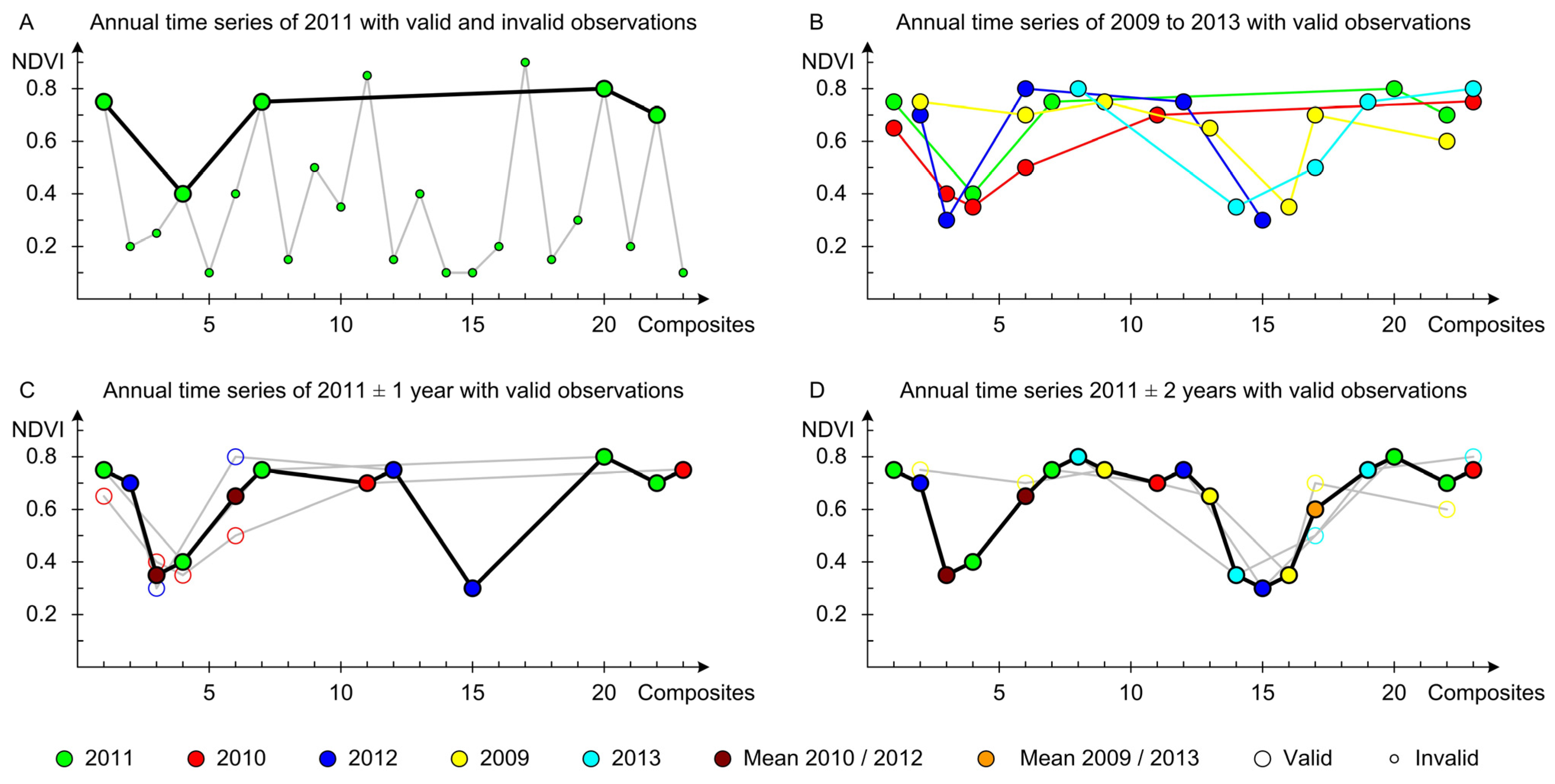
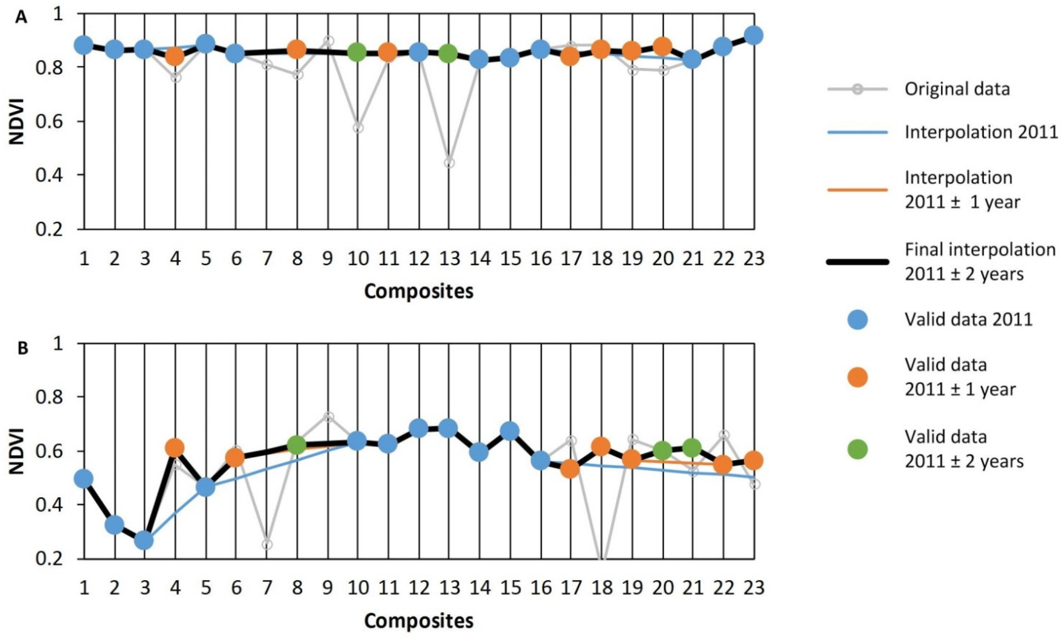
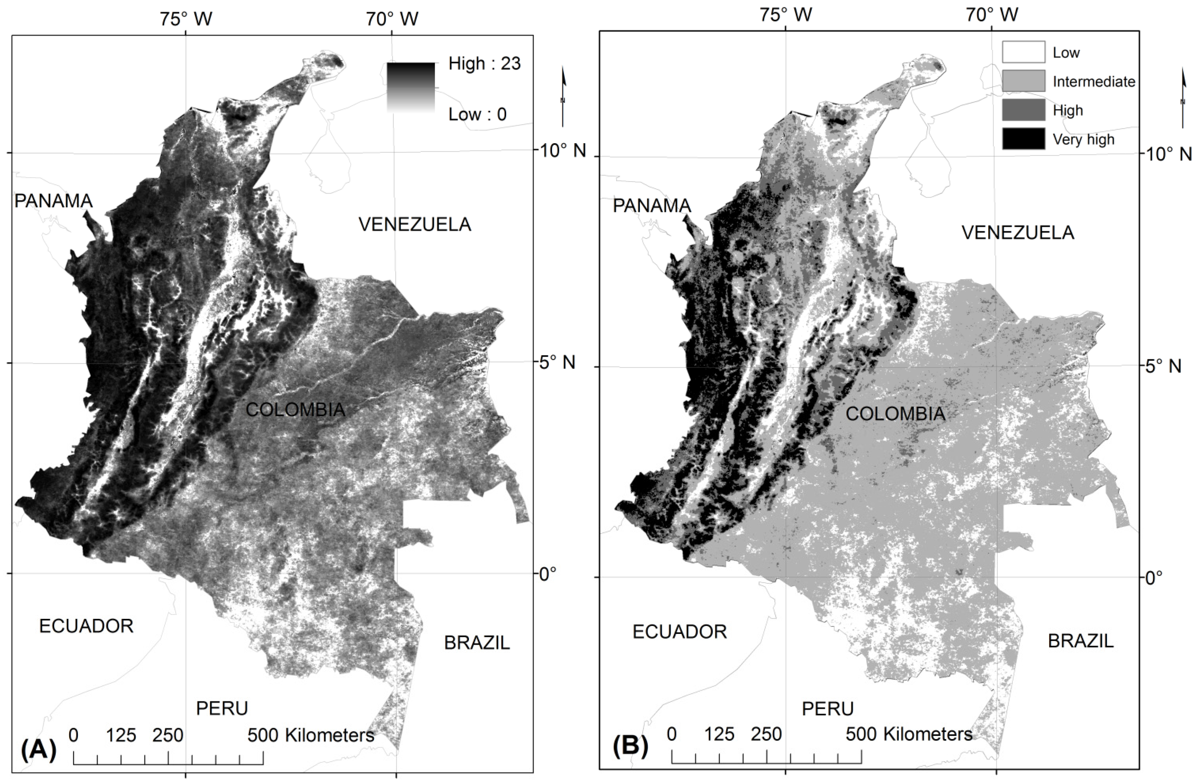
The high temporal resolution of MODIS with nearly daily observations in the tropics does not guarantee the existence of valid pixels in certain areas, mostly due to cloud formation. This study has shown that the number of invalid pixels in 2011 reduce by 54.5% when adding data from the previous and posterior year (2011 ± 1 year) and by 72.3% for 2011 ± 2 years. In addition, areas of no observations for the entire year 2011 (24,130 km²) reduced by 88% when integrating data from adjacent years (2011 ± 1 year) and by 94% for 2011 ± 2 years. This indicates that data integration over a longer period increases the possibility of valid data, thus aims at densification of information. The amount of valid pixels to be integrated from adjacent years into an annual time series will vary, e.g., due to the cloud content but will never be less than in the initial year. The effectiveness of this data integration approach may depend on the strength of seasonal dynamics; thus, land surface types with pronounced seasonal cycle, like deciduous forests, temperate grasslands, and croplands will benefit more than evergreen vegetation and barren areas. Therefore, we conclude that using a multi-year data integration is a viable approach for increasing the amount of valid data which is particularly useful for tropical and mountainous regions where cloud-free data is scarce.

Studies using daily MODIS data have shown that, for the year 2008, there were insufficient valid observations for 4.1% of the area of Colombia [6]. This same study, however, allowed temporal interpolation across several months, i.e., also performing image classification in area with just 3–4 valid observations for the entire year. Our results confirm these limitations of valid data availability (2.11%). Therefore, it will be difficult to implement recently-developed approaches for Landsat data [23,60] over Colombia as the simplest time series models require 12 valid observations.

The proposed multi-year data integration approach solves the difficulties of valid observations for a single year but is based on two important assumptions. First, it assumed that there are no notable temporal shifts among all years, such as a year with significantly earlier or later vegetation growth or differences in the magnitude of values in the time series, either due to natural variability, fire, or management in agricultural areas. Tests of temporal shifts, e.g., temporal cross-correlation [61,62,63], may be restricted by only having a few observations. The second prerequisite is that there is no land cover change. Thus, the method may not be used for generating annual land cover updates as it integrates source data from various years.

There could be several extensions and modifications to the approach as implemented in this study. For instance, data from more years could be integrated (Y_n ± 3, Y_n ± 4, Y_n ± 5, etc.) but it should be considered that the likelihood of land cover change increases with adding more years. A viable approach to obtain a land cover map for the nominally most recent year could only consider previous years, e.g., generating a map for 2013 may iteratively integrate data from 2012, 2011, and maybe 2010. An alternative to data integration for an invalid observation (as shown in this approach) is the calculation of the mean, regardless of an existing valid observation in the previous iteration. This, for instance, would modify the value of the composite 1 in Figure 1C to 0.7 instead of maintaining the value 0.75 from 2011. Instead of the proposed iterative approach that gives higher preference to Y_n ± 1 than Y_n ± 2, which more closely follows the logic of limiting the impact of possible land cover change in distant years, one could integrate data of multiple years all at once; thus, all have equal importance. For composite 6 with 0.65 (mean from 2010 and 2012) this approach would also include the value from 2009 resulting in 0.66. Another modification is the combination of this multi-year data integration approach with step-wise annual time series generation as described in Colditz et al. [21] that focuses on closing short data gaps which are not modified in following iterations, even if there is a valid value. For instance, an interpolation of gaps shorter or equal to two after the first round of data integration (Figure 1C) closes the gap between composites 12 and 15 and, thus, does not permit integrating composites 13 (2009) and 14 (2013) in Figure 1B.

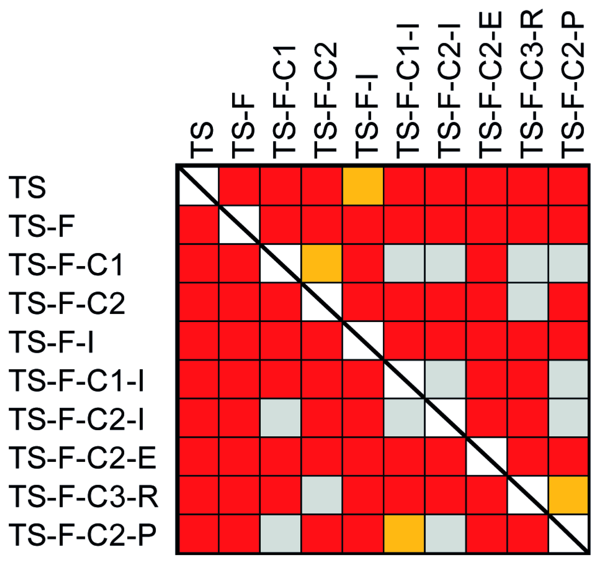
The comparison of land cover classifications based on various time series showed that the multi-year data integration approach as proposed in this study significantly improves map confidence and map accuracy. The Pacific region of Columbia, for instance, was highly favored using this approach shown by improving the classification of broadleaf forest. We recommend conducting further tests using this approach for vegetation and land cover classification, as well as for describing temporal dynamics in other tropical mountainous regions which suffer similar limitations with respect to cloud-free observations, such as in Central Africa and Indonesia. It also holds potential for other frequently cloud-covered areas such as temperate rain forests, e.g., in Western British Columbia, the Patagonian area of Chile, and the southern island of New Zealand.

Several regional to global land cover projects have integrated data of multiple years in order to increase data quality and fill periods of no available data [64,65,66] for a given year, but no study has quantitatively analyzed the impact of data integration on classification accuracy. The accuracy between the number of additional years used for compositing differed only marginally; confidence-based assessment showed best results for 2011 ± 1 year and error matrix-based accuracy assessment indicated a better performance for 2011 ± 2 years. As noted above, integration over even longer periods introduces uncertainty due to potential land cover change. It was also shown that filtering a single year for all invalid observations may have adverse effects on classification accuracy. The number of missing observations was too high to build a stable decision tree and boosting could not be invoked due to a too low accuracy of a single classifier [49].

Several other aspects may be considered to improve this result: training data may include mixed pixels to improve the classification of fragmented landscapes. A temporal match between reference data (to train and validate) and satellite data is desirable but difficult to achieve, as they are expensive to obtain and depend on specific sources or surveys. Some classes, such as páramo and secondary vegetation are defined from an ecosystem perspective and, thus, do not strictly link to land cover and have wide ambiguity in their interpretation which increases uncertainty in the map. The classification of cropland with coarse resolution data is difficult due to spatial, spectral, and temporal constraints which result in high errors. Most fields in tropical countries are smaller than a 500 m pixel. Crop types and agricultural practices vary on very small space, which causes a mix of the spectral and temporal signature. In the specific case of this study we found high ambiguity for coffee plantations as a sub-canopy crop along the Andes mountains, while palm oil, banana, and sugarcane are easily isolated in flat regions.

The addition of ancillary information only showed minor increases in accuracy for elevation and decreases when using other sources (precipitation, L-band radar data). This result may vary on the study area and classes to be classified, e.g., land cover classification of Colombia as a mountainous country can be improved with elevation data, while climatic gradients may be more helpful for countries with a high latitudinal range. Other tropical developing countries, rich in natural resources, with similar climatic characteristics may use these findings in order to assess land cover, understand the variables promoting land cover change and support sustainable development.

References

1. Anaya, J. Incendios en Colombia y Estimación de Emisión de Gases Efecto Invernadero por Quema de Biomasa; Sello Editorial. Universidad de Medellín: Medellín, Colombia, 2015; p. 168. [Google Scholar]
2. IDEAM. Leyenda Nacional de Coberturas de la Tierra. Metodología CORINE Land Cover Adaptada Para Colombia Escala 1:100.000; IDEAM: Bogotá, Colombia, 2010. [Google Scholar]
3. Eva, H.D.; Belward, A.; de Miranda, E.; di Bella, C.; Gond, V.; Huber, O.; Jones, S.; Sgrenzaroli, M.; Fritz, S. A land cover map of South America. Glob. Chang. Biol. 2004, 10, 731–744. [Google Scholar] [CrossRef]
4. Giri, C.; Long, J. Land cover characterization and mapping of South America for the year 2010 using Landsat 30 m satellite data. Remote Sens. 2014, 6, 9494–9510. [Google Scholar] [CrossRef]
5. Hojas, L.; Eva, H.D.; Gobron, N.; Simonetti, D.; Fritz, S. The application of medium-resolution MERIS satellite Data for continental land-cover mapping over South America: Results and caveats. In Remote Sensing of Land Use and Land Cover: Principles and Applications; Giri, C., Ed.; CRC/Taylor & Francis: Boca Ratón, FL, USA, 2012; pp. 325–337. [Google Scholar]
6. Blanco, P.D.; Colditz, R.R.; López Saldaña, G.; Hardtke, L.A.; Llamas, R.M.; Mari, N.A.; Fischer, A.; Caride, C.; Aceñolaza, P.G.; del Valle, H.F.; et al. A land cover map of Latin America and the Caribbean in the framework of the SERENA project. Remote Sens. Environ. 2013, 132, 13–31. [Google Scholar] [CrossRef]
7. Clark, M.L.; Aide, T.M.; Riner, G. Land change for all municipalities in Latin America and the Caribbean assessed from 250-m MODIS imagery (2001–2010). Remote Sens. Environ. 2012, 126, 84–103. [Google Scholar] [CrossRef]
8. Arino, O.; Bicheron, P.; Achard, F.; Latham, J.; Witt, R.G.; Weber, J.L. GlobCover—The Most Detailed Portrait of Earth; ESA Bulletin 136; ESA: Paris, France, 2008. [Google Scholar]
9. Bartholomé, E.; Belward, A.S. GLC2000: A new approach to global land cover mapping from Earth observation data. Int. J. Remote Sens. 2005, 26, 1959–1977. [Google Scholar] [CrossRef]
10. Friedl, M.A.; Sulla-Menashe, D.; Tan, B.; Schneider, A.; Ramankutty, N.; Sibley, A.; Huang, X. MODIS Collection 5 global land cover: Algorithm refinements and characterization of new datasets. Remote Sens. Environ. 2010, 114, 168–182. [Google Scholar] [CrossRef]
11. Hansen, M.C.; Defries, R.S.; Townshend, J.R.; Sohlberg, R. Global land cover classification at 1 km spatial resolution using a classification tree approach. Int. J. Remote Sens. 2000, 21, 1331–1364. [Google Scholar] [CrossRef]
12. Yu, L.; Wang, J.; Gong, P. Improving 30 m global land-cover map FROM-GCL with time series MODIS and auxiliary data sets: A segmentation-based approach. Int. J. Remote Sens. 2013, 34, 5851–5867. [Google Scholar] [CrossRef]
13. Leinenkugel, P.; Kuenzer, C.; Dech, S. Comparison and enhancement of MODIS cloud mask products for Southeast Asia. Int. J. Remote Sens. 2013, 34, 2730–2748. [Google Scholar] [CrossRef]
14. Hüttich, C.; Herold, M.; Wegmann, M.; Cord, A.; Strohbach, B.; Schmullius, C.; Dech, S. Assessing effects of temporal compositing and varying observation periods for large-area land-cover mapping in semi-arid ecosystems: Implications for global monitoring. Remote Sens. Environ. 2011, 115, 2445–2459. [Google Scholar] [CrossRef]
15. Kuenzer, C.; Dech, S.; Wagner, W. Remote sensing time series revealing land surface dynamics: Status quo and the pathway ahead. In Remote Sensing Time Series; Kuenzer, C., Dech, S., Wagner, W., Eds.; Springer: Heidelberg, Germany, 2015; pp. 1–24. [Google Scholar]
16. Chatfield, R. The Analysis of Time Series; CRC Press: Boca Raton, FL, USA, 2004. [Google Scholar]
17. Zhou, J.; Jia, L.; Menenti, M. Reconstruction of global MODIS NDVI time series: Performance of harmonic analysis of time series (HANTS). Remote Sens. Environ. 2015, 163, 217–228. [Google Scholar] [CrossRef]
18. Jönsson, P.; Eklundh, L. Seasonality extraction by function fitting to times-series of satellite sensor data. IEEE Trans. Geosci. Remote Sens. 2002, 40, 1824–1832. [Google Scholar] [CrossRef]
19. Jönsson, P.; Eklundh, L. TIMESAT—A program for analyzing time-series of satellite sensor data. Comput. Geosci. 2004, 30, 833–845. [Google Scholar] [CrossRef]
20. Colditz, R.R.; Conrad, C.; Wehermann, T.; Schmidt, M.; Dech, S. TiSeG: A flexible software tool for time-series generation of MODIS data utilizing the quality assessment science data set. IEEE Trans. Geosci. Remote Sens. 2008, 46, 3296–3308. [Google Scholar] [CrossRef]
21. Colditz, R.R.; Conrad, C.; Dech, S. Stepwise automated generation of time series using ranked data quality indicators. IEEE J. Sel. Top. Appl. Earth Obs. Remote Sens. 2011, 4, 272–280. [Google Scholar] [CrossRef]
22. Zhu, Z.; Woodcock, C.E. Automated cloud, cloud shadow, and snow detection in multitemporal Landsat data: An algorithm designed specifically for monitoring land cover change. Remote Sens. Environ. 2014, 152, 217–234. [Google Scholar] [CrossRef]
23. Zhu, Z.; Woodcock, C.E. Continuous change detection and classification of land cover using all available Landsat data. Remote Sens. Environ. 2014, 144, 152–171. [Google Scholar] [CrossRef]
24. Chen, L.; Jin, Z.; Michishita, R.; Cai, J.; Yue, T.; Chen, B.; Xu, B. Dynamic monitoring of wetland cover changes using time-series remote sensing imagery. Ecol. Inf. 2014, 24, 17–26. [Google Scholar] [CrossRef]
25. Chacon-Moreno, E.J. Mapping savanna ecosystems of the Llanos del Orinoco using multitemporal NOAA satellite imagery. Int. J. Appl. Earth Obs. Geoinf. 2004, 5, 41–53. [Google Scholar] [CrossRef]
26. Ganguly, S.; Friedl, M.A.; Tan, B.; Zhang, X.; Verma, M. Land surface phenology from MODIS: Characterization of the collection 5 global land cover dynamics product. Remote Sens. Environ. 2010, 114, 1805–1816. [Google Scholar] [CrossRef]
27. Hmimina, G.; Dufrêne, E.; Pontailler, J.Y.; Delpierre, N.; Aubinet, M.; Caquet, B.; de Grandcourt, A.; Burban, B.; Flechard, C.; Granier, A.; et al. Evaluation of the potential of MODIS satellite data to predict vegetation phenology in different biomes: An investigation using ground-based NDVI measurements. Remote Sens. Environ. 2013, 132, 145–158. [Google Scholar] [CrossRef]
28. Xiangming, X.; Hagen, S.; Zhang, Q.; Keller, M.; Moore-III, B. Detecting leaf phenology of seasonally moist tropical forests in South America with multi-temporal MODIS images. Remote Sens. Environ. 2006, 103, 465–476. [Google Scholar]
29. Yu, X.; Zhuang, D.; Chen, H.; Hou, X. Forest Classification based on MODIS time series and vegetation phenology. In Proceedings of 2004 IEEE International on Geoscience and Remote Sensing Symposium, Anchorage, AK, USA, 20–24 September 2004.
30. Jin, H.; Mountrakis, G.; Stehman, S.V. Assessing integration of intensity, polarimetric scattering, interferometric coherence and spatial texture metrics in PALSAR-derived land cover classification. ISPRS J. Photogramm. Remote Sens. 2014, 98, 70–84. [Google Scholar] [CrossRef]
31. Li, X.; Yeh, A.G. Multitemporal SAR images for monitoring cultivation systems using case-based reasoning. Remote Sens. Environ. 2004, 90, 524–534. [Google Scholar] [CrossRef]
32. Otukei, J.R.; Blaschke, T.; Collins, M. Fusion of TerraSAR-x and Landsat ETM+ data for protected area mapping in Uganda. Int. J. Appl. Earth Obs. Geoinf. 2015, 38, 99–104. [Google Scholar] [CrossRef]
33. Qi, Z.; Yeh, A.G.-O.; Li, X.; Zhang, X. A three-component method for timely detection of land cover changes using polarimetric SAR images. ISPRS J. Photogramm. Remote Sens. 2015, 107, 3–21. [Google Scholar] [CrossRef]
34. Thapa, R.B.; Itoh, T.; Shimada, M.; Watanabe, M.; Takeshi, M.; Shiraishi, T. Evaluation of ALOS PALSAR sensitivity for characterizing natural forest cover in wider tropical areas. Remote Sens. Environ. 2014, 155, 32–41. [Google Scholar] [CrossRef]
35. Hijmans, R.J.; Cameron, S.E.; Parra, J.L.; Jones, P.G.; Jarvis, A. Very high resolution interpolated climate surfaces for global land areas. Int. J. Climatol. 2005, 25, 1965–1978. [Google Scholar] [CrossRef]
36. UNODC. Monitoreo de Cultivos de Coca 2013. Available online: https://www.unodc.org/documents/crop-monitoring/Colombia/Colombia_Monitoreo_de_Cultivos_de_Coca_2013_web.pdf (accessed on 9 July 2015).
37. Etter, A.; McAlpine, C.; Wilson, K.; Phinn, S.; Possingham, H. Regional patterns of agricultural land use and deforestation in Colombia. Agric. Ecosyst. Environ. 2006, 114, 369–386. [Google Scholar] [CrossRef]
38. Poveda, G.; Waylen, P.R.; Pulwarty, R.S. Annual and inter-annual variability of the present climate in northern South America and southern Mesoamerica. Palaeogeogr. Palaeoclimatol. Palaeoecol. 2006, 234, 3–27. [Google Scholar] [CrossRef]
39. Olson, D.M.; Dinerstein, E.; Wikramanayake, E.D.; Burgess, N.D.; Powell, G.V.N.; Underwood, E.C.; D’Amico, J.A.; Itoua, I.; Strand, H.E.; Morrison, J.C.; et al. Terrestrial ecoregions of the world: A new map of life on earth. Bioscience 2001, 51, 933–938. [Google Scholar] [CrossRef]
40. Huete, A.; Didan, K.; Miura, T.; Rodriguez, E.P.; Gao, X.; Ferreira, L.G. Overview of the radiometric and biophysical performance of the MODIS vegetation indices. Remote Sens. Environ. 2002, 83, 195–213. [Google Scholar] [CrossRef]
41. Solano, R.; Didan, K.; Jacobson, A.; Huete, A. MODIS vegetation index user’s guide (MOD13 Series). Available online: http://vip.arizona.edu/documents/MODIS/MODIS_VI_UsersGuide_01_2012.pdf (accessed on 9 July 2015).
42. Loveland, T.R.; Belward, A.S. The international geosphere biosphere programme data and information system global land cover data set (DISCover). Acta Astronaut. 1997, 41, 681–689. [Google Scholar] [CrossRef]
43. Rincon, A.; Pascual, U.; Romero, M. An exploratory spatial analysis of illegal coca cultivation in Colombia using local indicators of spatial association and socioecological variables. Ecol. Indic. 2013, 34, 103–112. [Google Scholar] [CrossRef]
44. Myers, N.; Mittermeier, R.A.; Mittermeier, C.G.; da Fonseca, G.A.B.; Kent, J. Biodiversity hotspots for conservation priorities. Nature 2000, 403, 853–858. [Google Scholar] [CrossRef] [PubMed]
45. IAVH Institute. Aportes a la Conservación Estratégica de los Páramos de Colombia: Actualización de la Cartografía de los Complejos de Páramo a Escala 1:100.000. Available online: http://www.humboldt.org.co/es/noticias/actualidad/item/109-nueva-cartografia-de-los-paramos-de-colombia-diversidad-territorio-e-historia?highlight=YToxOntpOjA7czo3OiJwYXJhbW9zIjt9 (accessed on 9 July 2015).
46. Posada, F.; Barbosa, C.; Gutiérrez, H.; Yanine, D. Mapa de Coberturas Vegetales, uso y Ocupación del Espacio en Colombia. Available online: http://documentacion.ideam.gov.co/cgi-bin/koha/opac-detail.pl?biblionumber=29175&shelfbrowse_itemnumber=30478 (accessed on 9 July 2015).
47. Colditz, R.R.; López Saldaña, G.; Maeda, P.; Espinoza, J.A.; Tovar, C.M.; Hernández, A.V.; Benítez, C.Z.; Cruz López, I.; Ressl, R. Generation and analysis of the 2005 land cover map for Mexico using 250 m MODIS data. Remote Sens. Environ. 2012, 123, 541–552. [Google Scholar] [CrossRef]
48. Freund, Y.; Schapire, R.E. A decision-theoretic generalization of on-line learning and an application to boosting. J. Comput. Syst. Sci. 1997, 55, 119–139. [Google Scholar] [CrossRef]
49. Freund, Y.; Schapire, R.E. A short introduction to boosting. J. Jpn. Soc. Artific. Intell. 1999, 14, 771–780. [Google Scholar]
50. Foody, G.M. Status of land cover classification accuracy assessment. Remote Sens. Environ. 2002, 80, 185–201. [Google Scholar] [CrossRef]
51. Strahler, A.; Boschetti, L.; Foody, G.M.; Friedl, M.A.; Hansen, M.C.; Herold, M.; Mayaux, P.; Morisette, J.T.; Stehman, S.V.; Woodcock, C.E. Global Land Cover Validation: Recommendations for Evaluation and Accuracy Assessment of Global Land Cover Maps. Available online: http://cndwebzine.hcp.ma/cnd_sii/IMG/pdf/Document22222222222-17.pdf (accessed on 9 July 2015).
52. Quinlan, J.R. C4.5: Programs for Machine Learning; Morgan Kaufmann Publishers: Burlington, MA, USA, 1993. [Google Scholar]
53. Quinlan, J.R. Bagging, Boosting, and C4.5. Available online: http://www.cs.ecu.edu/~dingq/CSCI6905/readings/BaggingBoosting.pdf (accessed on 9 July 2015).
54. Colditz, R.R.; Schmidt, M.; Conrad, C.; Hansen, M.C.; Dech, S. Land cover classification with coarse spatial resolution data to derive continuous and discrete maps for complex regions. Remote Sens. Environ. 2011, 115, 3264–3275. [Google Scholar] [CrossRef]
55. Mogina, J.; Thongbai, P. Ecosystems and Human Well-Being: Multiscale Assessments: Findings of the Sub-Global Assessments Working Group, 2nd ed.; Island Press: Washington, DC, USA, 2015. [Google Scholar]
56. Colditz, R. An Evaluation of Different Training Sample Allocation Schemes for Discrete and Continuous Land Cover Classification Using Decision Tree-Based Algorithms. Remote Sens 2015, 7, 9655. [Google Scholar] [CrossRef]
57. Kissinger, G.M.; Herold, M.; de Sy, V. Drivers of Deforestation and Forest Degradation: A Synthesis Report for REDD+ Policymakers; The Government of the UK and Norway: Vancouver, BC, Canada, 2012. [Google Scholar]
58. Congalton, R.G.; Green, K. Assessing the Accuracy of Remotely Sensed Data, 2nd ed.; CRC Press: Boca Raton, FL, USA, 2009. [Google Scholar]
59. Foody, G.M. Thematic map comparison: Evaluating the statistical significance of differences in classification accuracy. Photogramm. Eng. Remote Sens. 2004, 70, 627–633. [Google Scholar] [CrossRef]
60. Zhu, Z.; Woodcock, C.E.; Holden, C.; Yang, Z. Generating synthetic Landsat images based on all available Landsat data: Predicting Landsat surface reflectance at any given time. Remote Sens. Environ. 2015, 162, 67–83. [Google Scholar] [CrossRef]
61. Colditz, R.R.; Llamas, R.M.; Ressl, R. Detecting change areas in Mexico between 2005 and 2010 using 250 m MODIS images. IEEE J. Selected Topics Appl. Earth Obs. Remote Sens. 2014, 7, 3358–3372. [Google Scholar] [CrossRef]
62. Lhermitte, S.; Verbesselt, J.; Verstraeten, W.W.; Coppin, P. A comparison of time series similarity measures for classification and change detection of ecosystem dynamics. Remote Sens. Environ. 2011, 115, 3129–3152. [Google Scholar] [CrossRef]
63. Colditz, R.R. On the day of observation in image composites and its impact on time series. IEEE J. Sel. Top. Appl. Earth Obs. Remote Sens. 2014, 7, 3350–3357. [Google Scholar] [CrossRef]
64. Bontemps, S.; Herold, M.; Kooistra, L.; van Groenestijn, A.; Hartley, A.; Arino, O.; Moreau, I.; Defourny, P. Revisiting land cover observation to address the needs of the climate modeling community. Biogeosciences 2012, 9, 2145–2157. [Google Scholar] [CrossRef] [Green Version]
65. Homer, C.; Huang, C.; Yang, L.; Wylie, B.; Michael, C. Development of a 2001 national land-cover database for the United States. Photogramm. Eng. Remote Sens. 2004, 70, 829–840. [Google Scholar] [CrossRef]
66. Radoux, J.; Lamarche, C.; van Bogaert, E.; Bontemps, S.; Brockmann, C.; Defourny, P. Automated training sample extraction for global land cover mapping. Remote Sens. 2014, 6, 3965–3987. [Google Scholar] [CrossRef]