Maize Leaf Area Index Retrieval from Synthetic Quad Pol SAR Time Series Using the Water Cloud Model

Abstract

In order to monitor crop growth along the season with synthetic aperture radar (SAR) images, radiative transfer models were developed to retrieve key biophysical parameters, such as the Leaf Area Index (LAI). The semi-empirical water cloud model (WCM) can be used to estimate LAI values from SAR data and surface soil moisture information. Nevertheless, instability problems can occur during the model calibration, which subsequently reduce its transferability in both time and space. To avoid these ill-posed cases, three calibration methodologies are benchmarked in the present study. The accuracy of the retrieved LAI values for each methodology was analyzed, as well as the sensitivity of the signal to LAI for different soil moisture values. The sensitivity of the cross-polarization was highlighted especially for high LAI. The VV polarization was found sensitive for LAI values inferior to 2 m${}^2$/m${}^2$. Given the differential sensitivity of the C-band backscatter to maize canopies in each polarization, a Bayesian fusion of the LAI estimates in linear polarizations was developed. This fusion gives lower weights to estimates with a high uncertainty. This method systematically reduces the error and its associated variance. When considering all polarizations, the RMSE on LAI estimation decreased by 0.32 m${}^2$/m${}^2$, i.e., one fourth of the error value, as compared to the best estimation from a single polarization, and the associated uncertainty was reduced by a factor of two. Focusing on the two most sensitive polarizations to maize canopies (VV-HV), the error diminished by a third. This fusion framework shows thus a great potential to improve the accuracy and reliability of LAI retrieval of C-band quad-polarized data, as well as dual-polarized data, such as Sentinel-1.

1. Introduction

The Leaf Area Index, a key parameter in crop growth and yield models, has been widely studied with remote sensing optical data [1,2,3]. However, its estimation from optical data is constrained by the presence of clouds. SAR systems are less susceptible to atmospheric effects and appears thus as a sensitive complementary solution. Crop growth monitoring often relies on radiative transfer models. Three main types of model exist: theoretical, empirical and semi-empirical models. Theoretical models simulate the radiative transfers based on electromagnetic mechanisms that account for the theoretical interactions of the electromagnetic signal with the crop (reflection, absorption, scattering). For radar, they describe the electromagnetic interactions of all canopy scattering elements (stems, leaves and ears) and the underlying soil surface [4]. Usually relying on complex equations, they require a large number of input parameters for describing the simulated target, which reduces their suitability for operational application. For instance, the fully-polarimetric model supported by the University of Tor Vergata (Rome) (UTOV) was first developed by Bracaglia et al. [5] and then further improved for agricultural applications [6]. Empirical relationships often relying on regressions of the backscattering coefficient to environmental parameters are widely used, but remain site and dataset specific [7]. Semi-empirical models are based on radiative transfer theory, but include simplification in formulas with fewer parameters and variables [8]. They aim at calculating the incoherent sum of the power backscattered by all considered scatterers and require in situ data to calibrate the model parameters. The canopy is represented by bulk variables, such as volumetric moisture, rather than a set of detailed canopy descriptors, like leaf size and orientation [9]. They can be easily inverted thanks to their simplicity, but they lack generalization capabilities [10].

As SAR backscattering is influenced by soil moisture, vegetation and soil roughness, the retrieval process is a so-called ill-posed problem: different combinations of soil moisture, vegetation and roughness can result in an identical signal [11]. Similarly, the ill-posedness of the inversion is a well-known issue in the optical domain [12,13]. Ill-posedness may result in unstable and inaccurate inversion performances if no regularization, i.e., constraints on the inverse solution, is applied [14]. To solve ill-posed problems, regularization techniques can be used to provide stable and reliable solutions (see [15] for an overview).

In this study, the model selected for maize LAI estimation is the semi-empirical water cloud model (WCM) [16], the most widely used for estimating LAI from SAR. The initial motivation was to improve the efficiency of empirical regression models without incorporating complex geometrically-based mathematical models of microwave-crop interaction [9]. The WCM has four main parameters: two related to canopy and two to the soil properties. Although easy to use, the WCM presents limitations, because it depends on multiple regressions for fitting its parameters. Each parameter has a physical interpretation, which cannot be easily explained using regression techniques [17]. Moreover, there is neither a standard implementation approach nor an a priori method for estimating its parameters [9]. Bouman et al. [18] mentioned as well that the parameter estimates can be highly correlated. As a result, different combinations of parameter values can lead to comparable model fits. This lack of stability in the WCM parameters has also been reported in other cases studies [10,19,20,21]. To avoid these limitations, different methodologies have been devised. For example, Xu et al. [22] used values from the literature. Svoray and Shoshany [23] estimated the two soil-related parameters from the generalized empirical VSMbackscatter model [24]. Champion et al. [25] and Moran et al. [26] carried out measurements over bare soils to calculate two soil parameters separately. Prevot et al. [10] determined the value of the parameter to the soil moisture based on an independent dataset. Graham and Harris [17] used a second-order radiative transfer scattering model (RT2) to calculate the values of two parameters of calibration. To reduce the empirical nature of the calibration dataset, Lucau-Danila [27] mixed in situ datasets with datasets generated by theoretical radiative transfer models that cover a wide range of situations. Kumar et al. [28] estimated the water cloud model vegetation parameters using a genetic algorithm. However, no published studies compared different methods of calibration of the WCM and their respective impact on the model stability and resulting accuracy.

The availability of SAR data has long constrained their use for crop growth monitoring, because yield forecasting requires frequent information during the whole growing season. More specifically, LAI retrieval at earlier stages of crop development can be very useful to estimate the sowing date, for instance, and, eventually, to calibrate crop growth models Moulin et al. [29]. With its systematic acquisition in large parts of the globe, the recently-launched C-SAR Sentinel-1 solves the problems related to image availability, since data are freely distributed. Hence, it is of utmost importance to benchmark calibration approaches and retrieval methodologies to reach the accuracy level required for operations. In this context, the objectives of this study are three-fold. First, the impact of different methodologies on the stability of the calibration of the WCM is evaluated to retrieving the crop-specific Leaf Area Index from SAR data. Throughout this paper, model instability refers to uncertainty in the uniqueness of the model parameters, which subsequently reduces the validity and, thus, transferability of the model in both space and time. Three different methodologies are implemented to calibrate the model, and their performances are compared in terms of parameter stability, backscattering coefficient simulation and LAI retrieval. These methodologies consist of: (i) calculating all calibration parameters simultaneously; (ii) setting one of the calibration parameters beforehand; or (iii) calculating separately the two calibration parameters that are related to the soil. This analysis was performed for all linear polarizations, i.e., VV, HH and HV. Second, the determination of the sensitivity of polarimetric responses to maize was analyzed under different soil moisture situations to investigate the sensitivity of the model at different levels of soil moisture and LAI. Finally, LAI estimates from linear polarizations were combined in a Bayesian framework to further improve the LAI estimation and to reduce its uncertainty.

2. Data

A synthetic dataset obtained from the theoretical UTOV model developed at the University of Rome [5] containing 72 variable combinations was used to calibrate the WCM. The UTOV model is based on a discrete approach of the radiative transfer theory and on the simulation of the microwave backscattering of soil and vegetation as a function of the sensor parameters and on the relevant biophysical parameters characterizing the observed surface. Vegetation elements are described as discrete dielectric scatterers, and suitable electromagnetic theories are used to compute their absorption and scattering cross-sections, as well as interactions, with soil and other scatterers. Vegetated areas are considered as a homogeneous half-space with a rough interface (representing the soil) overlaid by a single layer made up of the discrete dielectric scatterers. The first step of the modeling procedure consists of selecting suitable geometries for the vegetation elements and calculating their permittivity. Then, the extinction cross-sections and bistatic scattering cross-sections of the single elements are computed. Finally, single element contributions are combined to simulate the overall backscattering coefficient [30].

Simulated datasets allow exploring systematically all possible different combinations while controlling at the same time the scene parameters (including soil moisture condition). In this case, the UTOV model was specifically adjusted to maize using dedicated field measurements collected over Belgium [6,30]. The radar responses were simulated for a range of configurations proposed by C-band sensors as (∼5.3 GHz) ERS, ENVISAT and RADARSAT-2 over a maize growing season up to an LAI of 4 m${}^2$/m${}^2$ [30]. Simulations were systematically run for each incidence angle, ranging from 20° to 35° with a 5° step. Three conditions of top soil gravimetric water content were considered, i.e., dry (10% water content), medium (20%) and wet soil (30%). As soil roughness significantly impacts the backscattering coefficient only at earlier stages of plant growth, it was measured only at the beginning of the season. The bi-dimensional soil roughness was measured by photogrammetry following the method of Blaes et al. [31] and was estimated by its standard deviation and correlation length values, respectively 0.98 and 2.27 cm [30]. Each polarization has a specific response to canopy cover and water soil moisture (Figure 1). For instance, HH backscatter is only sensitive to LAI for low canopy covers (LAI < 2 m${}^2$/m${}^2$) and low soil moisture, whereas VH backscatter remains relatively sensitive to LAI whatever the soil moisture and canopy cover. An increase in the angle or in the crop LAI leads to (i) a reduced sensitivity to soil moisture and to (ii) a lower difference between VV and HH backscattering coefficients. At the beginning of the season, when the canopy cover is low, the temporal variations of the backscattering coefficient are mainly driven by soil moisture. For vegetated fields, on the contrary, similar signals are obtained whatever the soil water content. For this period, vegetation provides the main contribution to the backscattered signal; the soil influence becomes marginal. This soil moisture insensitivity is actually explained by a saturation of the signal. The higher sensitivity observed in the cross-polarization is due to a slower transition towards saturation of this particular polarization.

Figure 1. Average SAR backscatter profiles from the University of Tor Vergata (UTOV) dataset according to LAI for different soil moisture conditions in the (a) VV polarization, (b) HH polarization and (c) HV polarization. Confidence interval represent the standard deviation of the input data due to noise or variations in the acquisition angle. Soil moisture has a strong influence on the SAR backscatter when the crop cover is low (LAI < 3 m${}^2$/m${}^2$).

Figure 1. Average SAR backscatter profiles from the University of Tor Vergata (UTOV) dataset according to LAI for different soil moisture conditions in the (a) VV polarization, (b) HH polarization and (c) HV polarization. Confidence interval represent the standard deviation of the input data due to noise or variations in the acquisition angle. Soil moisture has a strong influence on the SAR backscatter when the crop cover is low (LAI < 3 m${}^2$/m${}^2$).

The outputs of the UTOV model were validated by comparing the simulated signal to measurements from different SAR sensors (ERS/SAR, ENVISAT/ASAR and RADARSAT-2). The validation dataset contained the four variables needed to calibrate the model, i.e., the LAI, the surface soil moisture ($V_m$), the SAR backscattering coefficient (${\sigma }^o$) and the local incidence angle (θ). The model reproduces fairly well the VV temporal trend with an RMSE of 1.2 dB [30]. A good correspondence was observed also for the cross-polarization, although only one date was simulated, because a single SAR image was acquired in cross-polarization. As far as the HH polarization was concerned, the model was in good agreement with the data until an LAI of 4 m${}^2$/m${}^2$. For a more detailed description of the validation of the UTOV data, the readers are referred to Blaes et al. [30].

3. Method

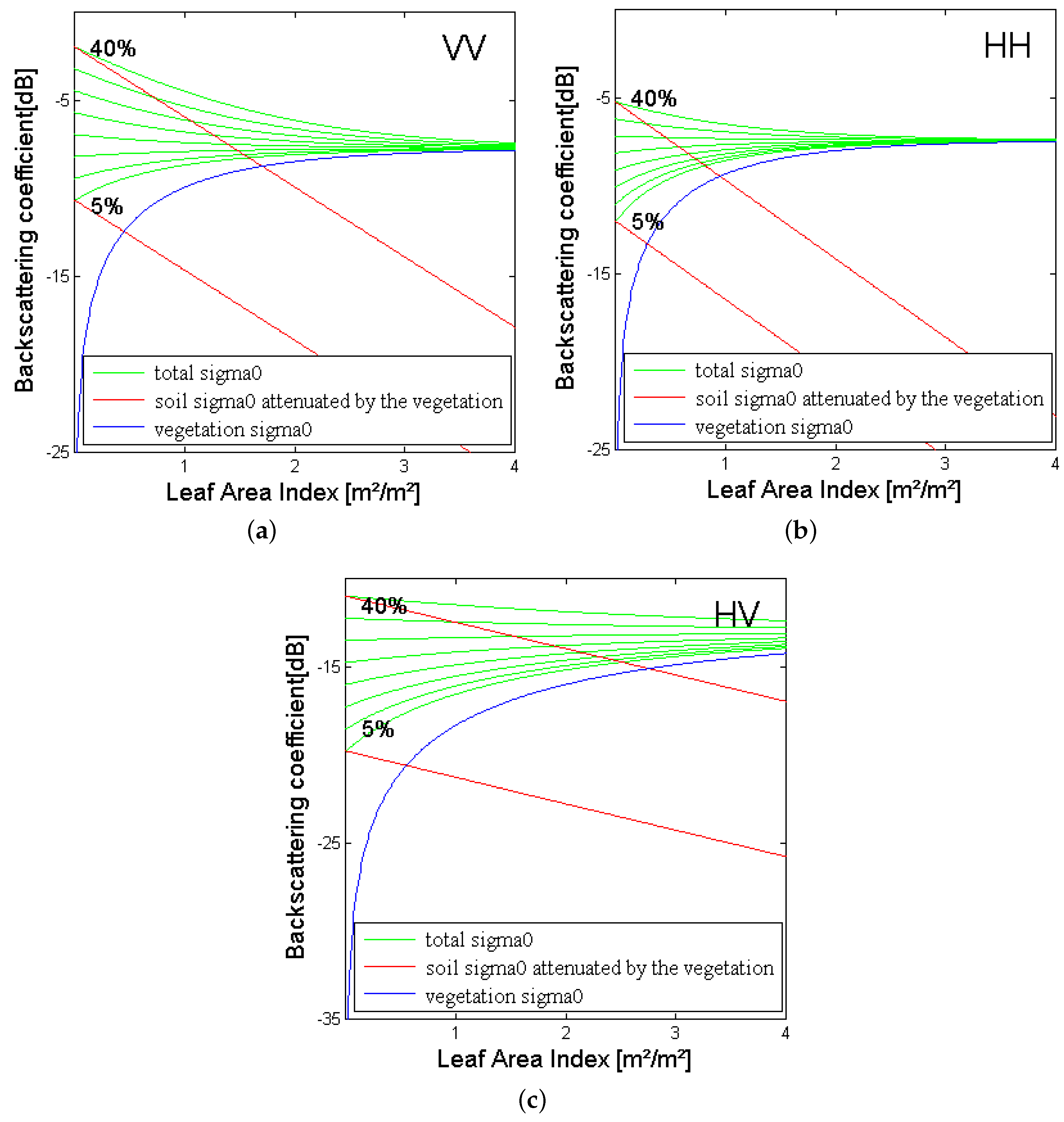
3.1. Water Cloud Model Implementation

The WCM [16] considers the vegetation canopy as a water cloud whose droplets are held in place by vegetation. The spherical droplets are of the same size and smaller than the wavelength. The basic form of the WCM can be written as:

$${\sigma }^o\left[m^2{m}^{-2}\right]=\frac{\sigma }{2Q}.\left[1-\text{exp}\left(\frac{-2.N.Q.h}{cos\theta }\right).cos\theta \right]+C.\text{exp}\left(D.V_m-\frac{2.N.Q.h}{cos\theta }\right).cos\theta$$

(1)

where ${\sigma }^o$ is the backscattering coefficient in power units (m${}^2$/m${}^2$) or the differential scattering cross-section (per unit area), which relates the magnitude of the power scattered to the power incident [32]. Parameters σ and Q are the radar cross-section (m${}^2$) and the total attenuation cross-section (m${}^2$) for one single particle, respectively, while N is the number of water particles per unit volume (m${}^{-3}$). The radar cross-section is a measure of the electromagnetic energy intercepted and re-radiated at the same wavelength by an object. $V_m$ is the volumetric surface soil moisture (kg/m${}^3$); h is the vegetation layer thickness (m); θ is the incidence angle (°). C and D are constant at a given frequency, polarization and soil surface roughness.

For the sake of simplicity, several assumptions are made. The cloud representing the vegetation consists of identical water particles, uniformly distributed throughout space according to a Poisson process. This implies that the plant biomass distribution in space is neglected. The only significant variables are cloud the height and cloud density, which are assumed to be proportional to the volumetric water content. As water particles are assumed identical in shape and size, ${\sigma }^o$ and Q are constant at a given frequency. A more common form of the WCM is thus:

$${\sigma }^o\left[m^2{m}^{-2}\right]=A.cos\theta .\left[1-\text{exp}\left(\frac{-B.W.h}{cos\theta }\right)\right]+C.\text{exp}\left(D.V_m-\frac{-B.W.h}{cos\theta }\right).cos\theta$$

(2)

where $\sigma /2.Q$ is replaced by A and $2.N.Q$ is replaced by $B.W$ in Equation (1); W is the water content per unit volume of the vegetation layer (kg/m${}^3$), and Bis a parameter. The model was further modified by Prevot et al. [10] to include the canopy descriptor variables $V_1$ and $V_2$:

$${\sigma }^o\left[m^2{m}^{-2}\right]=A.V_1^E.cos\theta \left[1-\text{exp}\left(\frac{-2.B.V_2}{cos\theta }\right)\right]+\text{exp}\left(\frac{-2.B.V_2}{cos\theta }\right).{10}^{(C.V_m-D)/10}$$

(3)

where E is a parameter present only in certain specific forms of the model [9]. The canopy descriptors $V_1$ and $V_2$ can be related to biophysical properties, such as LAI, the areal canopy moisture or the volumetric canopy moisture. In some studies [10,16,20,33,34,35], $V_1$ is set to 1. Parameter A relates to the backscatter from an optically-thick canopy at full cover, and parameter B acts as a canopy attenuation coefficient [9]. Parameter D is the radar backscatter from a perfectly dry soil, and the final parameter C relates to the sensitivity of the radar to variations in volumetric soil moisture. All of these parameters are dependent on the sensor configuration. In this study, $V_1$ was set to 1, and $V_2$ represents LAI. Therefore, the general formulation thus becomes:

$${\sigma }_{total}^o\left[m^2{m}^{-2}\right]={\sigma }_{veg}^o+t^2{\sigma }_{soil}^o$$

(4)

with:

$${\sigma }_{soil}^o\left[dB\right]=C.V_m-D$$

(5)

$${\sigma }_{veg}^o\left[m^2{m}^{-2}\right]=A.cos\theta .(1-t^2)$$

(6)

$$t^2=\text{exp}\left(\frac{-2B.LAI}{cos\theta }\right)$$

(7)

where $t^2$ is the two-way attenuation through the canopy. Theoretically, the rougher the surface, the larger ${\sigma }^o$ (due to an increased scattering); and the moister the soil, the larger ${\sigma }^o$ (due to a change in the soil dielectric constant). For a given roughness, the contribution of the soil to the backscattering coefficient is linked to the soil moisture as presented in Equation (5). The linear relationship between soil backscattering coefficient and volumetric surface soil moisture is based on experimental evidence indicating that the scattering coefficient of soil (expressed in dB) is approximately linearly related to the volumetric soil moisture content $V_m$ (kg/m${}^3$) [16]. This empirical relation needs to be calibrated for each soil type and roughness and for each sensor configuration, as well, i.e., C and D are functions of the frequency, the polarization configuration and the incidence angle.

3.2. Three Methodologies for Calibration

Three different methodologies were implemented and compared for calibrating the model:

• Methodology (i) aims at estimating the parameters A, B, C and D simultaneously using non-linear regression.
• For Methodology (ii), the soil relation was first fitted separately. The slope and intercept coefficients, i.e., parameters C and D, were calculated for a nearly bare soil (LAI = 0.08 m${}^2$/m${}^2$) using linear regression. Then, the two parameters related to the maize canopy (A and B) were calibrated using non-linear regression.
• In Methodology (iii), one of the soil calibration parameters, i.e., either C or D, is set using the value obtained in the second methodology, and the remaining parameters are then fitted simultaneously.

Methodology (iii) was implemented because strong positive correlations were observed between the two soil-related parameters while using the Methodology (i). High correlations mean that if one of these parameters increases, so does the other to obtain a comparable model fit. As a result, if one of these parameters is set, the other can be adjusted to obtain an appropriate model fit.

For all methodologies, the calibration parameters were estimated by non-linear regression. Non-linear regression relies on the minimization of the sum of squared deviations (SSD) between the UTOV data (in dB) and the corresponding simulated values (in dB). A global multilevel coordinate search (GMCS) optimization algorithm was implemented in sequential combination with the local Nelder–Mead simplex (NMS) algorithm [36]. The GMCS-NMS minimization algorithm facilitates the convergence towards a global minimum of the objective function, whereas the local NMS is more likely to be trapped in local minima. Calibrations and inversions of the model were done separately for each linear polarization: VV, HH and HV.

3.3. Model Inversion

The WCM inverse equation was used to estimate maize LAI from the backscattering coefficient, the local incidence angle and the surface soil moisture:

$$LA{I}_{sim}=\frac{cos\theta }{-2.B}.ln\left[\frac{{10}^{{\sigma }_{dB}^o/10}-A.cos\theta }{{10}^{(C.V_m-D)/10}-A.cos\theta }\right]$$

(8)

Identical SAR and soil properties were used for both calibration and inversion. Thresholds were defined for signal values falling outside the model prediction range; those signal values correspond to an LAI of 0.001 and 4 m${}^2$m${}^{-2}$, constraining the retrieval below 4. This threshold value was used as prior information because of the saturation effect of the SAR signal on plant development [37]. The error affecting the LAI values simulated by the WCM using SAR data was calculated thanks to a comparison with the reference LAI values of the calibration dataset. It should be noted that the retrieval was carried out in a leave-one-out fashion, so that the LAI retrieved was not used for model calibration.

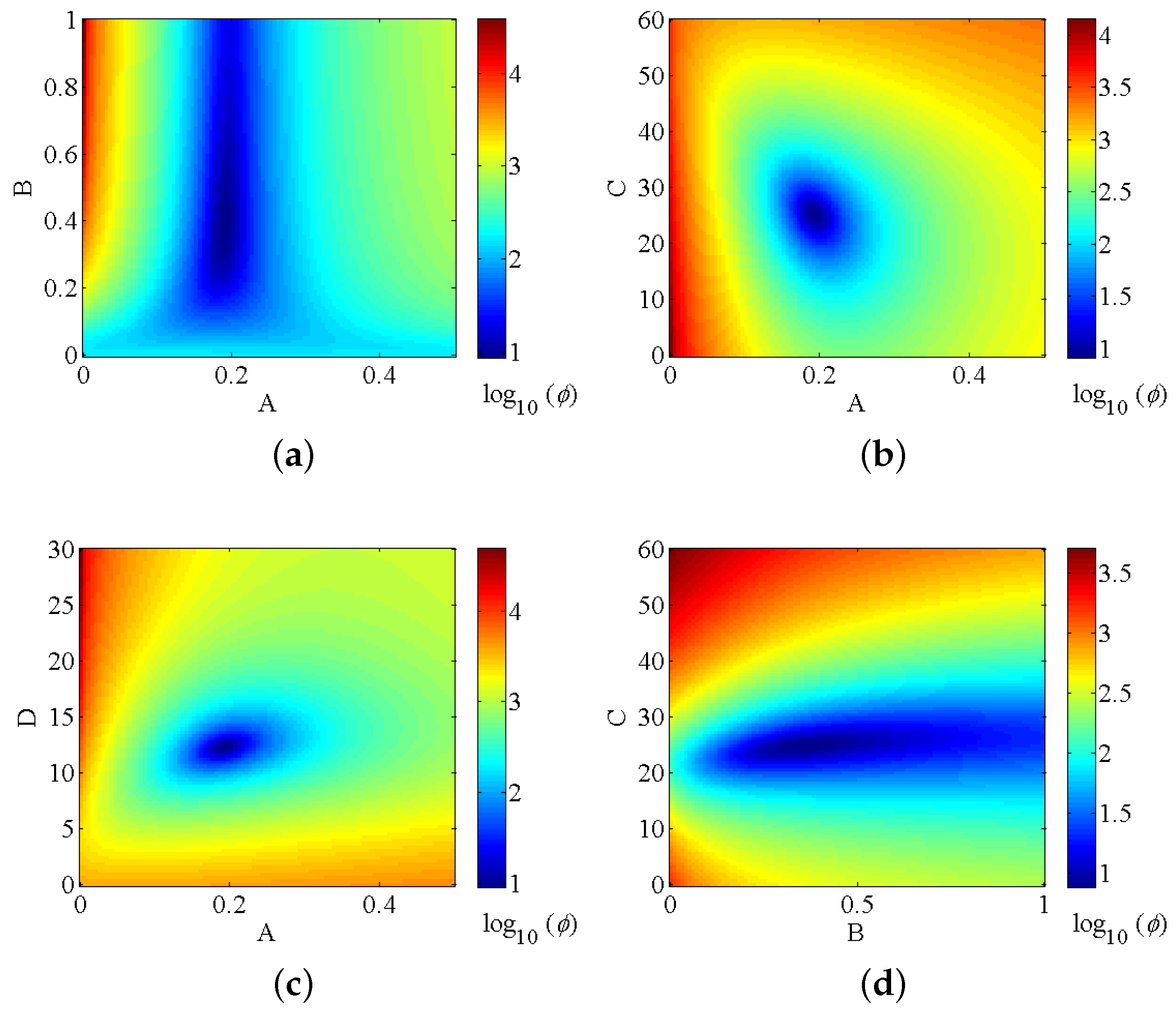
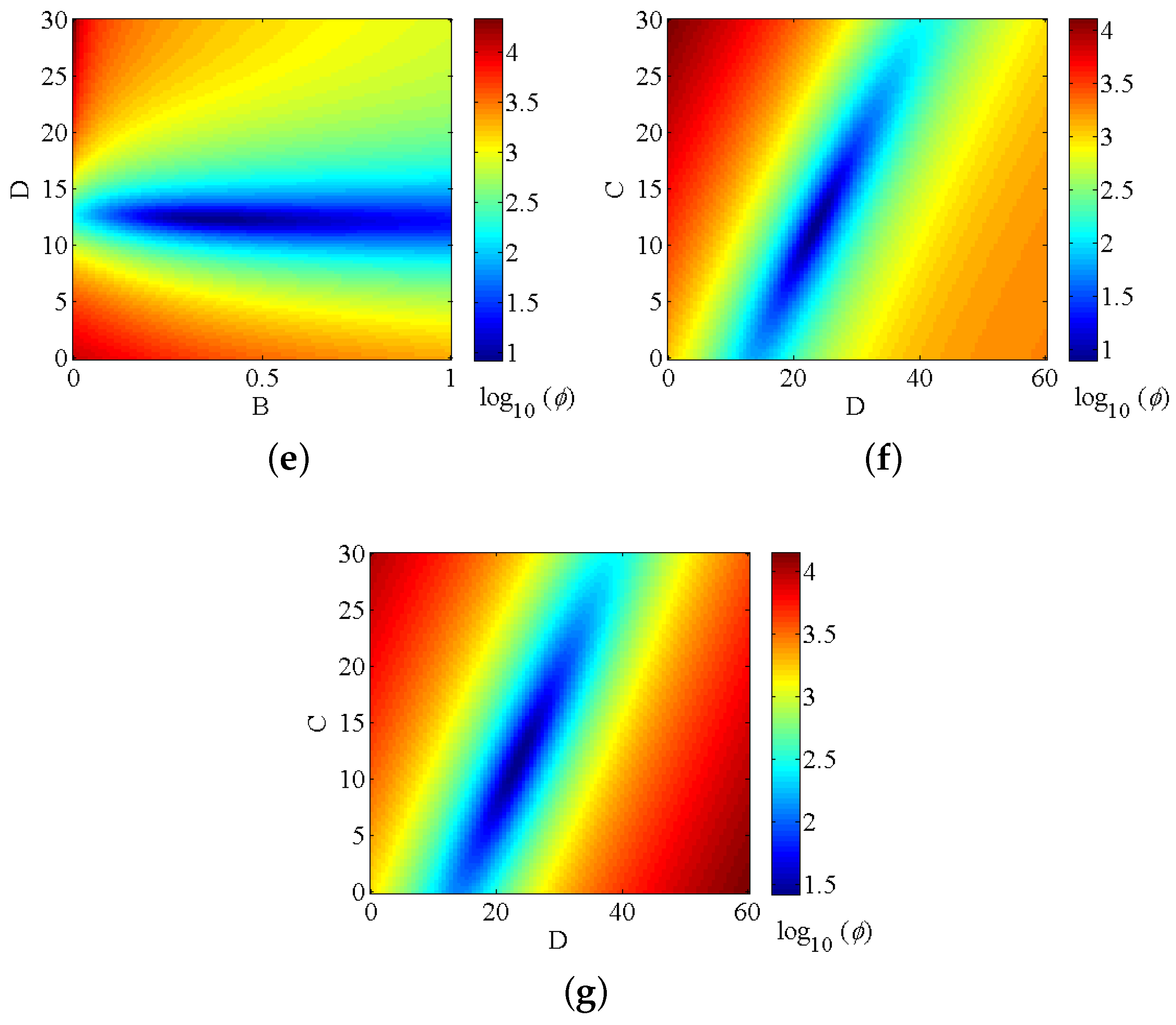
3.4. Analysis of the Calibration Process and Bayesian Fusion

Knowledge of the true distributions of the optimized parameters could have been obtained using the Monte Carlo method, for which many realizations of optimized parameter sets are generated from model fitting of data corrupted with measurement errors [38]. Nevertheless, this method requires high computing resources. Based on the Cramer–Rao theorem [39], the Hessian matrix gives a lower bound for the parameters covariance matrix ${\Sigma }_p$:

$${\Sigma }_p\ge H^{-1}$$

(9)

where H is the Hessian matrix. If the model were linear, the inequality of Equation (9) would become an equality, and the confidence region is an ellipsoid. Often, even non-linear models behave locally linearly, such that the ellipsoid gives a good approximate description of the actual confidence region [40]. Hence, the Hessian matrix results from the GMCS-NMS optimization and can be computed from the sensitivity of the model to its parameters, i.e., it is the square matrix of partial derivatives of the optimization function according to the calibration parameters [40]. The analysis of the resulting covariance and correlation matrices permits one to assess possible biases and instability problems in the calibration. In general, these issues are encountered in ill-posed problems and result in correlated parameters, leading to poor LAI estimation.

The SAR signal is influenced by soil moisture, vegetation and surface roughness. This effect makes the retrieval process a so-called “ill-posed” problem. In such problems, different combinations of soil moisture, vegetation and roughness can result in identical SAR signals.

To analyze the impact of the model instability on LAI retrieval, 1000 vectors of calibration parameters were simulated using their respective variance as approximated by the Hessian. The simulation of the parameters assumed a multivariate Gaussian assumption of the parameter distributions. LAI distributions were then computed for each variable combinations, and their corresponding standard deviations on LAI estimations were calculated. An input variable combination corresponds to a set of variables needed to calibrate the model, i.e., the LAI, $V_m$, σ^o and θ, which comes from the UTOV synthetic dataset. This technique provides thus a way of assessing the uncertainty associated with LAI estimates.

As the retrieved LAIs are now associated with a measure of their uncertainty, one could combine them, giving less weight to those estimates with high uncertainty, i.e., with large variances. Assuming those distributions as independent Gaussians, this was achieved in a Bayesian fusion framework [41]:

$${\text{LAI}}_{weighted}=\left(\frac{{\text{LAI}}_{VV}}{{\text{var}}_{VV}}+\frac{{\text{LAI}}_{HV}}{{\text{var}}_{HV}}+\frac{{\text{LAI}}_{HH}}{{\text{var}}_{HH}}\right)\times {\text{var}}_{weighted}$$

(10)

with:

$${\text{var}}_{weighted}={\left[\frac{1}{1/{\text{var}}_{VV}+1/{\text{var}}_{HV}+1/{\text{var}}_{HH}}\right]}^{-1}$$

(11)

and:

$${\text{std}}_{weighted}=\sqrt{{\text{var}}_{weighted}}$$

(12)

where ${\text{LAI}}_{weighted}$, ${\text{var}}_{weighted}$ and ${\text{std}}_{weighted}$ are the LAI obtained after Bayesian fusion and its corresponding variance and standard deviation; ${\text{LAI}}_{VV}$, ${\text{LAI}}_{HV}$, ${\text{LAI}}_{HH}$ and ${\text{var}}_{VV}$, ${\text{var}}_{VV}$, ${\text{var}}_{VV}$ are the LAI and the associated variance for each polarization.

4. Results

4.1. Impact of Three Calibration Methodologies on the Model Calibration and Inversion

The calibration and inversion were assessed for each polarization and calibration methodology by means of the coefficient of determination, the mean SSD, the mean absolute error (MAE), the root mean squared error (RMSE) and the bias between the original UTOV and the modeled WCM backscattering coefficient (Table 1). Regardless of the polarization, almost no difference was observed for the backscattering coefficient simulation of the different calibration methodologies. According to the MAE and RMSE, the VV polarization gave better results than the cross-polarization thanks to a better fit (lower SSD). The MAE, the RMSE and the bias between the estimated LAI and the reference LAI characterized the performance of the retrieval. The cross-polarization gave lower error on LAI estimation, with an MAE of 0.93 m${}^2$/m${}^2$. Nevertheless, only slight differences for the LAI retrieval were obtained for the different methodologies. Methodology (ii, in which both parameters C and D are set simultaneously, seems to increase the error of the cross-polarization performance. The error remains high in every case and could be explained by a low sensitivity of the signal to LAI for some specific soil moisture. However, one should bear in mind that such high RMSE LAIs are obtained from a synthetic dataset; the main interest of these results lies in the comparison of the calibration methodologies. Other studies found the cross-polarization as the best indicator of crop growth. For example, Ferrazzoli et al. [42] reported that C-HV polarization gives the maximum contrast between bare and vegetated soil, since even short vegetation provides an increase of the backscatter.

Table 1 also provides the mean, the minimum and the maximum standard deviations, as well as the confidence intervals (95%) obtained on LAI estimation for each methodology and each polarization. Mean standard deviations on LAI estimations were calculated by averaging all LAI standard deviations. The lowest standard deviations were obtained when both parameters C and D were calculated separately on nearly bare soils (Methodology (ii)); this was observed for each polarization. There were no significant differences between the standard deviation on LAI estimation when considering Methodologies (i) and (iii).

In addition to the respective performances for the different calibration methodologies, it was also of interest to investigate the stability of the values for the model parameters (Table 2). The Hessian matrix was used to evaluated the variances, coefficients of variation and correlation of the model parameters for each methodology and polarization. The value of parameter A remains almost constant from one calibration to another, while the three other parameters vary very slightly. The coefficients of variation for each parameter did not vary significantly according to the different methodologies of the calibration. The correlation between parameters C and D and between parameters A and B show higher correlation values for the cross-polarization, especially between the calibration parameters related to the vegetation. The correlations between parameters A and C, A and D, B and C and B and D are not presented, because they are largely inferior to those presented in the table. The high negative correlation between parameters A and B can be better understood looking at Equation (4). If either parameter A or B is high, so is the ${\sigma }_{veg}^o$ term of the WCM equation. A similar ${\sigma }_{veg}^o$ value can be obtained either with a calibrated model presenting low A and high B values or the opposite. The high negative correlation of these parameters is then encountered if the soil contribution is weak. Indeed, for a weak contribution of the soil to the signal (low ${\sigma }_{soil}^o$), the second term of Equation (3) is negligible, and ${\sigma }_{veg}^o$ explains mostly the SAR response. From the results and from the physical viewpoint, this means that the soil contribution is weak for HV polarization. High correlations (R${}^2$ > 0.93) were observed between the two calibration parameters related to the soil C and D. Gao et al. [43] highlighted a strong relationship between the HV cross-polarization and the volume scattering of the maize, which was mostly determined by the crown structure (especially LAI). Additionally, Moran et al. [44] concluded that the cross-polarization was particularly useful for monitoring both crop and soil conditions and was found to be the most insensitive to differences in sensor view direction and beam incidence angle. At shallow incidence angles, the sigma nought in HV polarization was the most sensitive to changes in vegetation structure with crop seasonal growth and harvest. More recently, with RADARSAT-2 quad-polarization SAR data, Jiao et al. [45] found correlations between cross-polarization backscatter and corn and soybean LAI.

Table 1. Results of the direct calibration and inversion of the water cloud model (WCM) for each polarization and after each methodology of calibration. RMSE on LAI estimation and associated mean, minimum and maximum standard deviations and intervals of confidence (95%) after calibration and inversion of the WCM.

		Direct Calibration					Inversion
	Methodology	R${}^{\mathbf{2}}$	SSD	MAE	RMSE	Bias	MAE	RMSE	Bias	Mean Std	Min Std	Max Std	IC
			(db)	(db)	(db)	(db)	(m${}^{\mathbf{2}}$/m${}^{\mathbf{2}}$)	(m${}^{\mathbf{2}}$/m${}^{\mathbf{2}}$)	(m${}^{\mathbf{2}}$/m${}^{\mathbf{2}}$)	(m${}^{\mathbf{2}}$/m${}^{\mathbf{2}}$)	(m${}^{\mathbf{2}}$/m${}^{\mathbf{2}}$)	(m${}^{\mathbf{2}}$/m${}^{\mathbf{2}}$)	(m${}^{\mathbf{2}}$/m${}^{\mathbf{2}}$)
VV	(i)	0.8	0.3	0.46	0.56	0	0.95	1.36	0.27	0.27	0.06	0.61	1.03
	(ii)	0.8	0.31	0.47	0.57	−0.01	0.96	1.37	0.28	0.17	0	0.44	0.67
	(iii) C set	0.8	0.31	0.47	0.57	0	0.96	1.36	0.28	0.25	0.05	0.52	1
	(iii) D set	0.8	0.31	0.47	0.56	0.01	0.96	1.36	0.28	0.22	0.03	0.44	0.87
HH	(i)	0.64	0.58	0.64	0.77	0	1.31	1.76	0.11	0.52	0.06	1.41	2.03
	(ii)	0.66	0.59	0.65	0.78	0.01	1.35	1.8	0.16	0.23	0	0.51	0.9
	(iii) C set	0.65	0.59	0.65	0.78	0	1.35	1.81	−0.17	0.6	0.05	1.61	2.35
	(iii) D set	0.66	0.59	0.65	0.78	0.02	1.34	1.8	0.15	0.59	0.03	1.57	2.32
HV	(i)	0.75	0.61	0.64	0.8	0	0.93	1.34	0.14	0.47	0.07	1.19	1.79
	(ii)	0.72	0.76	0.7	0.88	0.18	1.07	1.52	−0.3	0.21	0	0.5	0.81
	(iii) C set	0.75	0.63	0.64	0.8	0	0.91	1.3	0.1	0.32	0.06	0.68	1.27
	(iii) D set	0.75	0.62	0.64	0.8	0	0.93	1.34	0.14	0.43	0.02	1.24	1.67

Table 1. Results of the direct calibration and inversion of the water cloud model (WCM) for each polarization and after each methodology of calibration. RMSE on LAI estimation and associated mean, minimum and maximum standard deviations and intervals of confidence (95%) after calibration and inversion of the WCM.

		Direct Calibration					Inversion
	Methodology	R${}^{\mathbf{2}}$	SSD	MAE	RMSE	Bias	MAE	RMSE	Bias	Mean Std	Min Std	Max Std	IC
			(db)	(db)	(db)	(db)	(m${}^{\mathbf{2}}$/m${}^{\mathbf{2}}$)	(m${}^{\mathbf{2}}$/m${}^{\mathbf{2}}$)	(m${}^{\mathbf{2}}$/m${}^{\mathbf{2}}$)	(m${}^{\mathbf{2}}$/m${}^{\mathbf{2}}$)	(m${}^{\mathbf{2}}$/m${}^{\mathbf{2}}$)	(m${}^{\mathbf{2}}$/m${}^{\mathbf{2}}$)	(m${}^{\mathbf{2}}$/m${}^{\mathbf{2}}$)
VV	(i)	0.8	0.3	0.46	0.56	0	0.95	1.36	0.27	0.27	0.06	0.61	1.03
	(ii)	0.8	0.31	0.47	0.57	−0.01	0.96	1.37	0.28	0.17	0	0.44	0.67
	(iii) C set	0.8	0.31	0.47	0.57	0	0.96	1.36	0.28	0.25	0.05	0.52	1
	(iii) D set	0.8	0.31	0.47	0.56	0.01	0.96	1.36	0.28	0.22	0.03	0.44	0.87
HH	(i)	0.64	0.58	0.64	0.77	0	1.31	1.76	0.11	0.52	0.06	1.41	2.03
	(ii)	0.66	0.59	0.65	0.78	0.01	1.35	1.8	0.16	0.23	0	0.51	0.9
	(iii) C set	0.65	0.59	0.65	0.78	0	1.35	1.81	−0.17	0.6	0.05	1.61	2.35
	(iii) D set	0.66	0.59	0.65	0.78	0.02	1.34	1.8	0.15	0.59	0.03	1.57	2.32
HV	(i)	0.75	0.61	0.64	0.8	0	0.93	1.34	0.14	0.47	0.07	1.19	1.79
	(ii)	0.72	0.76	0.7	0.88	0.18	1.07	1.52	−0.3	0.21	0	0.5	0.81
	(iii) C set	0.75	0.63	0.64	0.8	0	0.91	1.3	0.1	0.32	0.06	0.68	1.27
	(iii) D set	0.75	0.62	0.64	0.8	0	0.93	1.34	0.14	0.43	0.02	1.24	1.67

Table 2. Values of the parameters obtained for each methodology and each polarization, along with their associated variances, coefficients of variation and correlation as derived by means of the Hessian matrix.

	Methodology	A	VarA	${\mathbf{CV}}_{\mathbf{A}}$	B	Var B	${\mathbf{CV}}_{\mathbf{B}}$	C	Var C	${\mathbf{CV}}_{\mathbf{C}}$	D	Var D	${\mathbf{CV}}_{\mathbf{D}}$	Corr(C,D)	Corr(A,B)
VV	(i)	0.19	∼0	0.016	0.43	0.002	0.10	25.7	2.12	0.06	12.1	0.1	0.03	0.93	0.14
	(ii)	0.19	∼0	0.015	0.38	0.001	0.08	20.9	-	-	11.7	-	-	0.93	0.21
	(iii) C set	0.19	∼0	0.016	0.39	0.001	0.09	20.9	-	-	11.6	0.01	0.01	-	0.13
	(iii) D set	0.19	∼0	0.016	0.40	0.001	0.09	23.7	0.27	0.02	11.7	-	-	-	0.1
HH	(i)	0.2	∼0	0.025	0.38	0.004	0.17	20.4	4.25	0.10	13.1	0.22	0.04	0.94	−0.56
	(ii)	0.2	∼0	0.025	0.34	0.003	0.16	17.1	-	-	12.3	-	-	0.93	−0.6
	(iii) C set	0.2	∼ 0	0.026	0.34	0.003	0.16	17.1	-	-	12.4	0.03	0.01	-	−0.58
	(iii) D set	0.2	∼0	0.026	0.34	0.003	0.16	17.2	0.48	0.04	12.3	-	-	-	−0.59
HV	(i)	0.06	∼0	0.08	0.12	0.0005	0.19	22.3	3.22	0.08	20.4	0.17	0.02	0.94	−0.92
	(ii)	0.05	∼0	0.04	0.15	0.0005	0.14	19.8	-	-	20.7	-	-	0.93	−0.77
	(iii) C set	0.07	∼0	0.09	0.10	0.0004	0.19	19.8	-	-	19.8	0.02	0.01	-	−0.93
	(iii) D set	0.06	∼0	0.07	0.13	0.0004	0.16	23.6	0.38	0.03	20.7	-	-	-	−0.91

Table 2. Values of the parameters obtained for each methodology and each polarization, along with their associated variances, coefficients of variation and correlation as derived by means of the Hessian matrix.

	Methodology	A	VarA	${\mathbf{CV}}_{\mathbf{A}}$	B	Var B	${\mathbf{CV}}_{\mathbf{B}}$	C	Var C	${\mathbf{CV}}_{\mathbf{C}}$	D	Var D	${\mathbf{CV}}_{\mathbf{D}}$	Corr(C,D)	Corr(A,B)
VV	(i)	0.19	∼0	0.016	0.43	0.002	0.10	25.7	2.12	0.06	12.1	0.1	0.03	0.93	0.14
	(ii)	0.19	∼0	0.015	0.38	0.001	0.08	20.9	-	-	11.7	-	-	0.93	0.21
	(iii) C set	0.19	∼0	0.016	0.39	0.001	0.09	20.9	-	-	11.6	0.01	0.01	-	0.13
	(iii) D set	0.19	∼0	0.016	0.40	0.001	0.09	23.7	0.27	0.02	11.7	-	-	-	0.1
HH	(i)	0.2	∼0	0.025	0.38	0.004	0.17	20.4	4.25	0.10	13.1	0.22	0.04	0.94	−0.56
	(ii)	0.2	∼0	0.025	0.34	0.003	0.16	17.1	-	-	12.3	-	-	0.93	−0.6
	(iii) C set	0.2	∼ 0	0.026	0.34	0.003	0.16	17.1	-	-	12.4	0.03	0.01	-	−0.58
	(iii) D set	0.2	∼0	0.026	0.34	0.003	0.16	17.2	0.48	0.04	12.3	-	-	-	−0.59
HV	(i)	0.06	∼0	0.08	0.12	0.0005	0.19	22.3	3.22	0.08	20.4	0.17	0.02	0.94	−0.92
	(ii)	0.05	∼0	0.04	0.15	0.0005	0.14	19.8	-	-	20.7	-	-	0.93	−0.77
	(iii) C set	0.07	∼0	0.09	0.10	0.0004	0.19	19.8	-	-	19.8	0.02	0.01	-	−0.93
	(iii) D set	0.06	∼0	0.07	0.13	0.0004	0.16	23.6	0.38	0.03	20.7	-	-	-	−0.91

The uniqueness of the calibration parameters’ optimum was also investigated using response surfaces of the objective function. Response surfaces are two-dimensional contour plots representing the objective function as a function of two calibration parameters, while other parameters are kept constant at their optimal value. This analysis partly highlights the core of the calibration procedure, such as the presence of a well-defined solution or local minima and, also, qualitatively, parameter sensitivities and correlations. The response surfaces of the optimization were extracted for the VV polarization when using Methodology (i). For Figure 2a–e, each response surface shows a well-defined global minimum corresponding to the optimal parameter values. This illustrates the uniqueness of the solution in the A–B, A–C, A–D, B–C and B–D parameter planes. Yet, for the B–A and B–D parameter pairs, less well-defined minima can be observed, especially with respect to B. Figure 2f shows a significant positive correlation between parameters C and D. This stems from the fact that a similar soil contribution signal can be obtained for either high or low B and C parameters. Parameters C and D are the soil calibration parameters; the correlation between these parameters can be explained by the mathematical linear function linking them; similar results can be obtained either with high or low values of both parameters C and D. Their correlation shows that an endless number of solutions may exist for these two parameters. Such correlation and limited parameter sensitivities result inherently in large uncertainties in the estimation of these parameters. This is also observed when fitting the soil relationships alone with nearly bare soil observations (Figure 2g), which further highlights the dependency of the soil parameter values, which was addressed by the development of different calibration methodologies. Similarly to what was observed in Table 2, no strong dependence of the response surfaces on the methodology was observed.

Figure 2. Response surface of the objective function in the (a) A–B, (b) A–C, (c) A–D, (d) B–C, (e) B–D and (f) C–D plans for the first calibration methodology for the VV polarization; (g) the C–D plan when fitting the soil relation alone with nearly bare soil observation for the VV polarization.

Figure 2. Response surface of the objective function in the (a) A–B, (b) A–C, (c) A–D, (d) B–C, (e) B–D and (f) C–D plans for the first calibration methodology for the VV polarization; (g) the C–D plan when fitting the soil relation alone with nearly bare soil observation for the VV polarization.

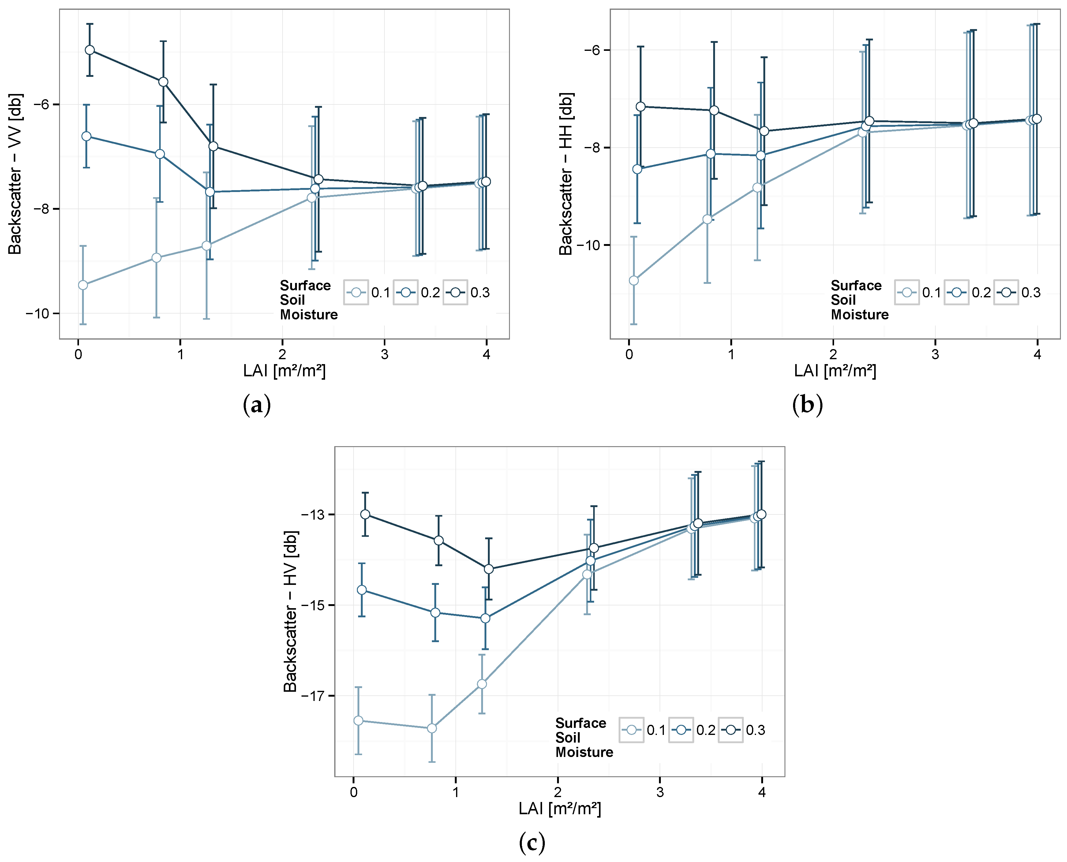
4.2. Insensitivity of the Signal to LAI at Specific Soil Moisture Levels

The charts in Figure 3 show the backscatter for each polarization as a function of LAI for different soil moisture contents after WCM calibration. This allows identifying which polarization is the most suitable for LAI estimation according to the canopy and soil moisture conditions. For the two co-polarizations, the backscattered signal of observations with intermediate soil moisture values is only slightly sensitive to LAI compared to soil moisture. Indeed, looking at the VV polarization, the signal spans over less than 1 dB between LAI values of 0–4 m${}^2$/m${}^2$ when soil moisture is equal to 20%, on the one hand. However, it spans over 4 dB when soil moisture is either very low (5%) or very high (40%). Regarding the cross-polarization, the backscattering coefficient is less sensitive to LAI when the soil moisture is high. In this case, the signal varies within less than 1 dB for LAI values of 0–4 m${}^2$/m${}^2$ when soil moisture is equal to 35% and within nearly 7 dB when soil moisture is very low (5%). Moreover, the signal becomes insensitive to LAI at high LAI values. This is observed especially for the HH polarization, for which the signal amplitude is less than 1 dB from LAI equal to three to LAI equal to 4 m${}^2$/m${}^2$, whatever the soil moisture condition.

This saturation effect has been already shown by Brisco and Brown [37]. Similarly, McNairn et al. [46] reported that the information on crop condition provided by C-band SAR can be limited due to signal saturation. In that study, when the maize canopy reaches a height of about 1 m, the C-HH backscattering response saturates. Ferrazzoli et al. [47] found that the C-HH and C-VV backscattering response increases with LAI, but the signal saturates once the LAI reaches a value of 2–3 m${}^2$/m${}^2$. Inoue et al. [48] identified the correlation expressed by exponential curves of both the Leaf Area Index and leaf biomass ${\sigma }^o$ throughout all growth stages, although ${\sigma }^o$ saturates around an LAI of 3 m${}^2$/m${}^2$. Although saturation is problematic when these canopies accumulate significant biomass, information on the soil and crop conditions is still available early in the season. Early information is the most needed from a crop yield forecasting perspective. Furthermore, this saturation appears less significant with the C-HV backscatter signal. The smaller errors on LAI estimation obtained for HV polarization were probably due to the less drastic saturation effect of the signal with plant development.

Figure 3. Backscattering coefficient simulation according to different soil moisture conditions and canopy statuses after WCM calibration for the VV (a), HH (b) and HV (c) polarizations. The green curves represent the total backscattering at different soil moisture values (from 5%–40% by steps of 5%). The red curve represents the backscattering coefficient from the soil attenuated by the vegetation for soil moisture of 5% and 40%. The blue curve represents the vegetation backscattering coefficient.

Figure 3. Backscattering coefficient simulation according to different soil moisture conditions and canopy statuses after WCM calibration for the VV (a), HH (b) and HV (c) polarizations. The green curves represent the total backscattering at different soil moisture values (from 5%–40% by steps of 5%). The red curve represents the backscattering coefficient from the soil attenuated by the vegetation for soil moisture of 5% and 40%. The blue curve represents the vegetation backscattering coefficient.

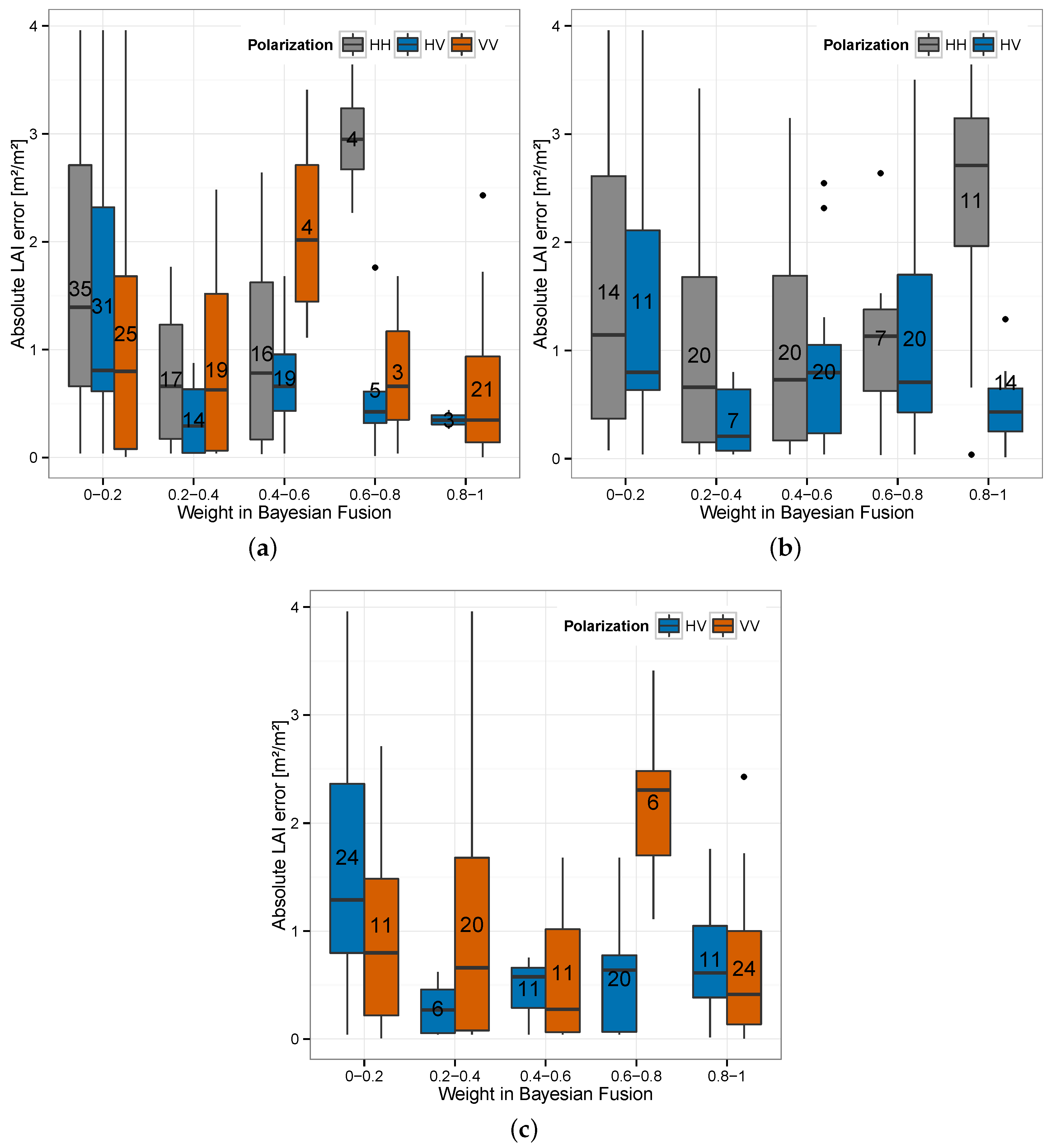
4.3. Bayesian Fusion of LAI Estimates

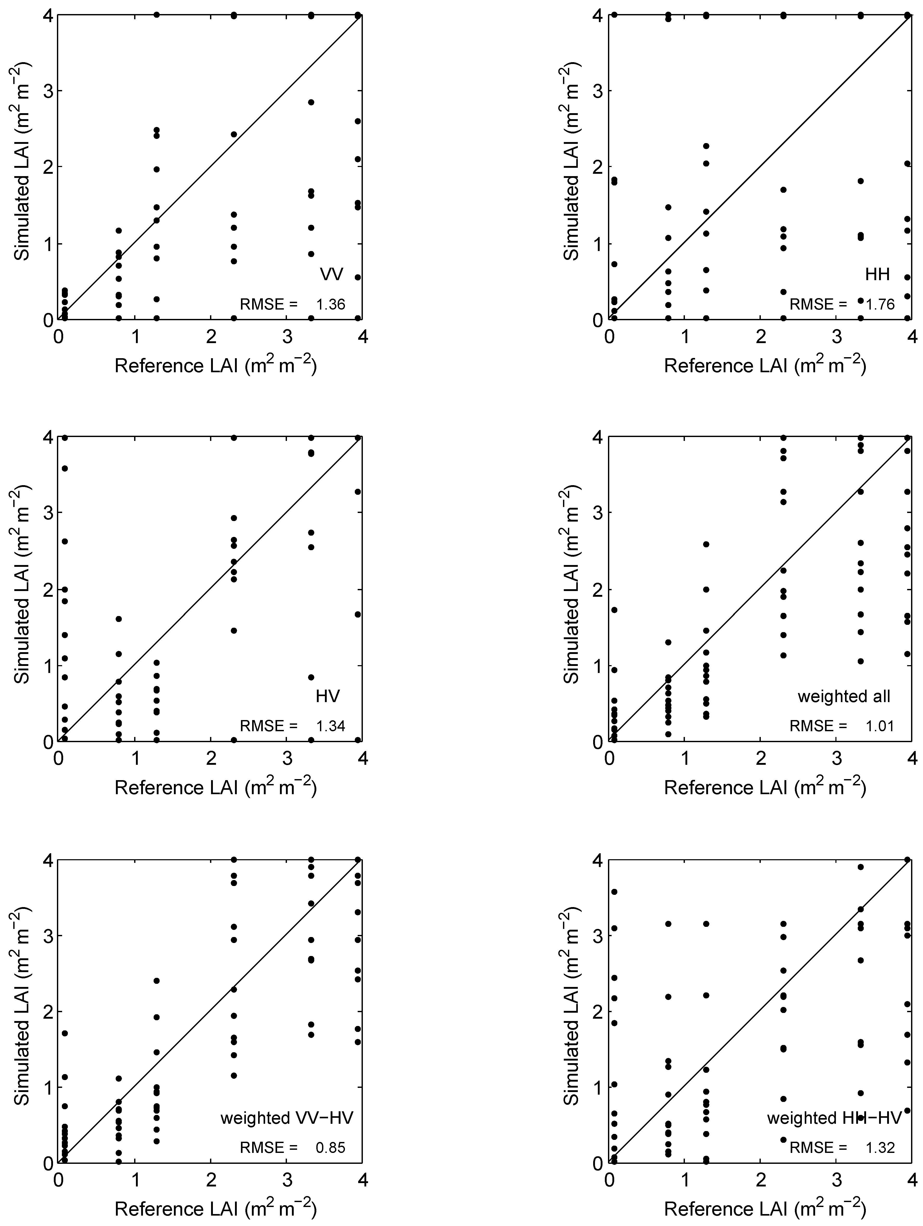
An LAI recalculation capitalizing on all polarizations was proposed following a Bayesian fusion framework. This appears especially sensitive as (1) both LAI estimation error and uncertainty were high with single linear polarization and as (2) the model suffers from instability problems. LAIs retrieved from linear polarization were combined to give LAI estimates by using Equations (10)–(12), for computing the fused LAI and its standard deviation (Figure 4). Three fusion cases were investigated. The first case considers estimates derived from all polarizations, whereas the other two focus on dual fusion (VV-HV and HH-HV).

Considering first single-polarization retrievals, the VV polarization seems to be more appropriate for small LAI estimation (under 1 m${}^2$/m${}^2$), but none of the three polarizations gives a robust estimation for the entire LAI range. Out-of-range values are to be related to signal saturation, the insensitivity of the signal to specific soil moisture levels or LAI, as well as the effects of the acquisition angle, as discussed in the previous section (see also Beriaux et al. [49]).

Figure 4. Reference LAI versus simulated LAI, after water cloud model inversion using VV, HH and HV polarizations and after LAI recalculation by weighting VV, HH and HV retrieved LAI (n = 72).

Figure 4. Reference LAI versus simulated LAI, after water cloud model inversion using VV, HH and HV polarizations and after LAI recalculation by weighting VV, HH and HV retrieved LAI (n = 72).

When fusing all three polarizations, RMSE on LAI estimation decreased by 0.32 m${}^2$/m${}^2$, i.e., one fourth of the error value of the best estimation resulting from a single polarization (Table 3). This RMSE is significantly different from the RMSE obtained on LAI estimation using whatever single polarization according to a Fisher–Snedecor statistical test (significance level of 0.01). Moreover, the standard deviation after the Bayesian fusion is at least twice smaller than the one obtained using a single polarization.

Table 3. The performance of the retrieval with single polarization and after Bayesian LAI recalculation. With all three polarizations, the RMSE on LAI estimation decreased by 0.32 m${}^2$/m${}^2$, whereas considering only the VV-HV polarizations, the RMSE drops by 0.49 m${}^2$/m${}^2$.

Polarization	RMSE on LAI (m${}^2$m${}^{-2}$)	Std on LAI (m${}^2$m${}^{-2}$)	R${}^2$
Single pol
VV	1.36	0.27	0.38
HH	1.76	0.52	0.13
HV	1.34	0.47	0.38
Quad pol
weighted	1.02	0.13	0.56
Dual pol
weighted HH/HV	1.32	0.32	0.30
weighted VV/HV	0.85	0.16	0.67

Table 3. The performance of the retrieval with single polarization and after Bayesian LAI recalculation. With all three polarizations, the RMSE on LAI estimation decreased by 0.32 m${}^2$/m${}^2$, whereas considering only the VV-HV polarizations, the RMSE drops by 0.49 m${}^2$/m${}^2$.

Polarization	RMSE on LAI (m${}^2$m${}^{-2}$)	Std on LAI (m${}^2$m${}^{-2}$)	R${}^2$
Single pol
VV	1.36	0.27	0.38
HH	1.76	0.52	0.13
HV	1.34	0.47	0.38
Quad pol
weighted	1.02	0.13	0.56
Dual pol
weighted HH/HV	1.32	0.32	0.30
weighted VV/HV	0.85	0.16	0.67

Three elements explain the under-performance of the quad pol fusion compared to the VV-VH fusion. First, the conditional independence hypothesis is more likely to be violated with three polarizations than with two. Second, by adding a variable, there is an transfer of the weights to the third variable even if the associated variance is very large comparatively. Finally, even if the weight associated with an unreliable estimate is small, its contribution to the final weighted LAI might still be significant if its value strongly differ from the true LAI value. The last two points are particularly valid when one of the variable is noisy and has a low sensitivity to the parameter of interest. Bayesian fusion is thus a powerful tool, especially if utilized with prior knowledge of the sensitivity of the polarizations.

The underlying assumption of the Bayesian fusion is that the larger the variance of the estimates, the larger their associated error. A priori, as uncertain simulated values should be more affected by errors, they should have smaller weights. Conversely, LAIs retrieved with low uncertainty should have larger weights, as they are expected to have a higher accuracy. This assumption has been tested and verified (Figure 5). In all three cases, low weights correspond to high absolute error. High absolute errors are also observed especially for intermediate to high weights, but as the number of observations is low, their mean absolute LAI error might be overestimated. When considering all polarizations (Figure 5(a)), HH, the less sensitive polarization, never reaches weights superior to 0.6, which demonstrates the relevance of the variance estimation by the Hessian.

Combining VV and VH provides the best results, which is interesting, as dual pol images are then sufficient to improve the LAI retrieval and the computation time is reduced. The VV signal reacts more to vertical targets, thus to stems, while the HH signal interacts with horizontal elements less numerous in a maize field: objects having linear features of a size comparable to the wavelength or more tend to cause larger reflections when the polarization alignment agrees with their structural alignment [50].

Figure 5. (a–c) Weight attributed to a simulation in a given polarization and its corresponding retrieval error in absolute values.

Figure 5. (a–c) Weight attributed to a simulation in a given polarization and its corresponding retrieval error in absolute values.

5. Discussions

The three different methodologies for model calibration lead to very similar models, which implies that the errors obtained remain similar, as well. The main differences were the coefficients of variation and the correlations of the parameters, as well as the standard deviations of estimated LAI. High correlations between the two calibration parameters C and D related to the soil were observed for Methodologies (i) and (ii). Methodology (i) consisted of calculating all calibration parameters simultaneously, while Methodology (ii) fixed one of the calibration parameters beforehand. These correlations emphasize the inter-dependency of the parameters due to the non-uniqueness of the model [11]: different combinations of parameter values lead to comparable results. Considering this fact, Methodology (iii) should be more appropriate to ensure the stability of the model. This methodology consisted of calculating separately two calibration parameters that are related to the soil. Nevertheless, Methodology (iii) does not seem to decrease the uncertainty associated with the LAI estimation (see Table 1). Close or higher standard deviations are obtained in comparison with the other methodologies. Methodology (ii) seems the most appropriate to reduce the standard deviation on LAI estimation, but its RMSE is often higher than for other methodologies. In fact, no methodology simultaneously improves the LAI estimation and reduces its associated uncertainty for all polarizations. This only occurs in the cross-polarization for Methodology (iii), in which the trend of the linear relationship of the soil is set. Thus, the WCM suffers from instability whatever the methodology, which suggests that the calibration data strongly influence the parameter values and, thus, its generalization capabilities. Besides, Methodologies (ii) and (iii) require prior soil information: observations over bare soils are mandatory or parameters must be set according to the literature. Finding appropriate values is not an easy task as they are a function of the soil type and the sensor configuration, i.e., the wavelength, the polarization and the incidence angle.

The same kind of theoretical polarimetric analysis could be performed for different sensor configurations, in term of frequency and incidence angle, to help to determine which configurations are the most convenient to assess the vegetation growth. SAR polarimetry analysis could also allow determining the best polarization configuration for crop parameter extraction, including synthesized polarizations, i.e., elliptical or oblique polarizations. It should be emphasized here that this study focused on a WCM with specific values for the canopy descriptors, $V_1=1$ and $V_2=$ LAI, as proposed by Ulaby et al. [20]. The framework developed here remains valid for other frequencies, crop types and canopy descriptors with different impacts on the retrieval accuracy and model stability. High LAI values are hardly assessable, because of the saturation effect encountered for maize [49]. Special care should be paid when inverting the model on independent datasets for which no prior information about the LAI is available. In this case, if the model inversion gives LAI values of 4 m${}^2$/m${}^2$ or higher, these values have to be discarded. When the C-band saturates, one could switch to longer wavelengths, such as the L-band, as it has more penetration through the canopy for higher biomass. In this respect, the future L-band SAOCOM mission could certainly be considered for the retrieval of high values of LAI.

To overcome the instability limitation of the model, as well as to combine the differential sensitivities of each polarization, a Bayesian recalculation of the LAI based on the retrieval uncertainty was carried out. It successfully improved the LAI estimation, but reduced its associated uncertainty. Yet, the efficiency of the fusion varies according to the polarizations considered. When considering all polarizations, the RMSE on LAI estimation decreased by 0.32 m${}^2$/m${}^2$, i.e., one fourth of the error value, as compared to the best estimation from a single polarization. The associated uncertainty was reduced by a factor of two. Marginal improvements were achieved combining HH-HV estimates, which seems logical given the insensitivity of HH backscatter to maize canopy. On the contrary, the VV-HV fusion provided the best results: the errors were reduced by a third and the uncertainty by half. The performance of the VV-HV fusion is particularly encouraging for maize crop growth monitoring with SAR data, as the Sentinel-1 main operational imaging mode, the interferometric wide-swath mode [51], is provided VV-VH [52]. Though such results were obtained with a thoroughly validated synthetic dataset, they should be further confirmed using actual measurements.

The accuracy obtained in this study is similar to what can be found in the radar literature. Xu et al. [22] tested and fitted several versions of the WCM for the sugar beet crop using ERS-1 SAR C-band images with simultaneous ground truth data in a few parcels; they obtained an accuracy of 0.5–1 m${}^2$/m${}^2$ on LAI estimation. A similar analysis was carried out by Auquière [53] and on several maize crop fields and C-band VV SAR data; the author obtained mean absolute errors on LAI estimation varying from 0.44–0.96 m${}^2$/m${}^2$. For the same crop, Lucau-Danila [27] retrieved LAI from multi-sensors and multi-year SAR data at the C-band through the WCM with an RMSE of 0.44 m${}^2$/m${}^2$, excluding fields with specific soil moisture. Dabrowska-Zielinska et al. [34] extracted LAI among other parameters C- and L-bands images with a mean error of 0.66 m${}^2$/m${}^2$. Prevot et al. [10] retrieved wheat LAI from ground-based scatterometer data at C-band and X-band through the WCM with an error of 1 m${}^2$/m${}^2$ on LAI estimates. Compared to what is usually achieved in the optical domain, the error obtained with optical data falls in the range of 0.3–1 m${}^2$/m${}^2$ generally [3,54,55,56,57], especially if regularization constraints are applied [1,55]. The range of 15%–20% is regarded by Baret et al. [58] as the currently achievable accuracy for LAI from remote sensing observations. In fact, the Global Climate Observing System (GCOS) recommends that the error on LAI retrieval falls within ±0.5 LAI unit [59]. While LAI derived from optical data tend to satisfy this requirement, LAI retrieval from SAR data still needs further improvements to reach the ±0.5 LAI unit target. The approach proposed in this study is to turn the ill-posed problem into uncertainty for each polarization, which is thus combined using a Bayesian framework. Further improvements of the inversion process require more information to be exploited, including better radiative transfer models, the exploitation of proper prior information on the distribution of canopy and atmospheric variables and knowledge of the uncertainties in satellite measurements, as well as possible spatial and temporal constraints [60].

A direct consequence of using synthetic data is that soil moisture was known a priori. To transpose the current approach with actual measurements, one would be required to estimate soil moisture before starting to retrieve LAI, as it is an input of the WCM. A first possibility is to use globally-available products derived from remote sensing or data assimilation, such as the Soil Moisture Operational Products System (SMOPS), the ECMWF (European Centre for Medium-Range Weather Forecasts) numerical weather prediction system (SM-DAS-2, a surface soil moisture product produced by the European Centre for Medium Range Weather Forecasts Land Data Assimilation System), ASCAT (Advanced Scatterometer) and SMOS (Soil Moisture Ocean Salinity), and that have been already validated (see Albergel et al. [61]). For crop monitoring, however, the spatial resolution of those products tends to remain too coarse [62]. An alternative to cope with the coarse spatial resolution is to derive surface-soil moisture directly from the SAR data used for the LAI retrieval [10,63,64]. Finally, Bériaux et al. [62] tackled the issues related to soil influence on the SAR signal in monitoring maize crop growth using the WCM. Two methods to assess surface-soil moisture were explored. The first method was based on ground-penetrating radar and the second on a hydrological model, the soil, water, atmosphere and plant (SWAP) model [65], with which the surface-soil moisture level can be estimated as a function of time. The latter method was tested with two types of input meteorological data: ground meteorological data and estimated meteorological data. The authors demonstrated that both soil moisture levels estimated by the SWAP model and soil permittivity measured by ground-penetrating radar can be successfully used for retrieving maize LAI values from SAR data with the water cloud model.

6. Conclusions and Perspectives

Three different methodologies were compared in order to calibrate the WCM in the perspective of retrieving maize LAI from quad-polarized SAR data. These methodologies were implemented using a synthetic dataset to find the one to further improve the model fit and reduce the uncertainty on LAI estimation. Results show that no best methodology was found when both stability of the model and uncertainty on LAI estimation are taken into account. An analysis of the SAR polarimetric response of the maize fields highlighted that the sensitivity of the SAR signal to maize growth for different soil moisture levels differs from one polarization to another. This observation is of great interest because it allows determining the best polarization for a given soil moisture situation. As polarizations convey complementary information and because of the measurement uncertainty and the ill-posed inverse problem, a Bayesian fusion based on all polarizations improved the LAI retrieval and reduced its uncertainty by a factor of two. Furthermore, the results combining three linear polarizations are very promising, but the method cannot be applied in situations where polarized SAR data are unavailable. Indeed, polarimetric data are linked to images covering smaller areas than dual- or single-polarized data, while the large swath can prevail for large region applications. The same kind of theoretical polarimetric analysis could be done for different sensor configurations, in terms of frequency and incidence angle and for different crop types, with the aim of identifying which configurations are the most sensitive to the crop development for the observed situations. As this study relied on synthetic data, future work should confirm these results with real remote sensing data for further validations.

Three scenarios are possible for implementing this research’s results. First, if no prior information is available on the backscatter sensitivity to LAI, a Bayesian fusion based on all polarizations would improve the LAI retrieval and reduce its uncertainty by a factor of two. Nevertheless, only some SAR sensors can systematically acquire scenes in multi-polarization modality. Furthermore, polarimetric data are linked to images covering smaller areas than dual- or single-polarized data, while the large swath can prevail for large region applications. Second, when the sensitivity of the polarizations is known, dual-polarized images, including one co- and one cross-polarization, can be combined to enhance the retrieval quality and reduce its uncertainty. Discarding the polarization with less sensitivity further supports the enhancement of the retrieval as noisy information is set aside. Besides, dual pol images can be seen as a good trade-off between the number of polarizations and the swath. For instance, Sentinel-1 is the first C-band radar satellite to systematically image over Europe in a 12-day repeat cycle with a swath of 250-km in dual polarization. The rest of the globe has an evolving acquisition plan in terms of coverage and acquisition mode. Finally, if only single-polarized images are available, these findings allow determining situations for which model inversion cannot provide reliable LAI estimates.

References

1. Atzberger, C. Object-based retrieval of biophysical canopy variables using artificial neural nets and radiative transfer models. Remote Sens. Environ. 2004, 93, 53–67. [Google Scholar] [CrossRef]
2. Pasolli, L.; Asam, S.; Castelli, M.; Bruzzone, L.; Wohlfahrt, G.; Zebisch, M.; Notarnicola, C. Retrieval of Leaf Area Index in mountain grasslands in the Alps from MODIS satellite imagery. Remote Sens. Environ. 2015, 165, 159–174. [Google Scholar] [CrossRef]
3. Li, W.; Weiss, M.; Waldner, F.; Demarez, V.; Hagolle, O.; Baret, F. A Generic Algorithm to Estimate LAI, FAPAR and FCOVER Variables from SPOT4_HRVIR and Landsat Sensors: Evaluation of the Consistency and Comparison with Ground Measurements. Remote Sens. 2015, 7, 15494–15516. [Google Scholar] [CrossRef]
4. Fung, A. Microwave Scattering and Emission Models and Their Applications; Artech House: Boston, MA, USA, 1994; pp. 1–592. [Google Scholar]
5. Bracaglia, M.; Ferrazzoli, P.; Guerriero, L. A fully polarimetric multiple scattering model for crops. Remote Sens. Environ. 1995, 54, 170–179. [Google Scholar] [CrossRef]
6. Della Vecchia, A.; Ferrazzoli, P.; Guerriero, L. Modelling microwave scattering from long curved leaves. Waves Random Media 2004, 14, S333–S343. [Google Scholar] [CrossRef]
7. Hoekman, D.H.; Quinones, M.J. P-band SAR for optical forest mapping and land cover change. Earth Obs. Q. 1999, 61, 18–22. [Google Scholar]
8. Richards, J. Radar backscatter modelling of forests: A review of current trends. Int. J. Remote Sens. 1990, 11, 1299–1312. [Google Scholar] [CrossRef]
9. Graham, A.; Harris, R. Extracting biophysical parameters from remotely sensed radar data: A review of the water cloud model. Prog. Phys. Geogr. 2003, 27, 217–229. [Google Scholar] [CrossRef]
10. Prevot, L.; Champion, I.; Guyot, G. Estimating surface soil moisture and leaf area index of a wheat canopy using a dual-frequency (C and X bands) scatterometer. Remote Sens. Environ. 1993, 46, 331–339. [Google Scholar] [CrossRef]
11. Bertoldi, G.; Della Chiesa, S.; Notarnicola, C.; Pasolli, L.; Niedrist, G.; Tappeiner, U. Estimation of soil moisture patterns in mountain grasslands by means of SAR RADARSAT2 images andhydrological modeling. J. Hydrol. 2014, 516, 245–257. [Google Scholar] [CrossRef]
12. Combal, B.; Baret, F.; Weiss, M.; Trubuil, A.; Mace, D.; Pragnere, A.; Myneni, R.; Knyazikhin, Y.; Wang, L. Retrieval of canopy biophysical variables from bidirectional reflectance: Using prior information to solve the ill-posed inverse problem. Remote Sens. Environ. 2003, 84, 1–15. [Google Scholar] [CrossRef]
13. Jacquemoud, S.; Baret, F. Estimating Vegetation Biophysical Parameters by Inversion of a Reflectance Model on High Spectral Resolution Data; INRA: Versailles, France, 1993; pp. 339–350. [Google Scholar]
14. Durbha, S.S.; King, R.L.; Younan, N.H. Support vector machines regression for retrieval of leaf area index from multiangle imaging spectroradiometer. Remote Sens. Environ. 2007, 107, 348–361. [Google Scholar] [CrossRef]
15. Baret, F.; Buis, S. Estimating canopy characteristics from remote sensing observations: Review of methods and associated problems. In Advances in Land Remote Sensing; Springer: Berlin, Germany, 2008; pp. 173–201. [Google Scholar]
16. Attema, E.; Ulaby, F.T. Vegetation modeled as a water cloud. Radio Sci. 1978, 13, 357–364. [Google Scholar] [CrossRef]
17. Graham, A.; Harris, R. Estimating crop and waveband specific water cloud model parameters using a theoretical backscatter model. Int. J. Remote Sens. 2002, 23, 5129–5133. [Google Scholar] [CrossRef]
18. Bouman, B.; van Kraalingen, D.; Stol, W.; van Leeuwen, H. An agroecological modeling approach to explain ERS SAR radar backscatter of agricultural crops. Remote Sens. Environ. 1999, 67, 137–146. [Google Scholar] [CrossRef]
19. Bouman, B.; Goudriaan, J. Estimation of crop growth from optical and microwave soil cover. Int. J. Remote Sens. 1989, 10, 1843–1855. [Google Scholar] [CrossRef]
20. Ulaby, F.; Allen, C.; Eger, G.; Kanemasu, E. Relating the microwave backscattering coefficient to leaf area index. Remote Sens. Environ. 1984, 14, 113–133. [Google Scholar] [CrossRef]
21. Van Leeuwen, H. Methodology for Combining Optical and Microwave Remote Sensing in Agricultural Crop Monitoring. Ph.D. Thesis, Wageningen Agricultural University, Wageningen, The Netherlands, 1996. [Google Scholar]
22. Xu, H.; Steven, M.; Jaggard, K. Monitoring leaf area of sugar beet using ERS-1 SAR data. Int. J. Remote Sens. 1996, 17, 3401–3410. [Google Scholar] [CrossRef]
23. Svoray, T.; Shoshany, M. SAR-based estimation of areal aboveground biomass (AAB) of herbaceous vegetation in the semi-arid zone: A modification of the water-cloud model. Int. J. Remote Sens. 2002, 23, 4089–4100. [Google Scholar] [CrossRef]
24. Shoshany, M.; Svoray, T.; Curran, P.; Foody, G.M.; Perevolotsky, A. The relationship between ERS-2 SAR backscatter and soil moisture: Generalization from a humid to semi-arid transect. Int. J. Remote Sens. 2000, 21, 2337–2343. [Google Scholar] [CrossRef]
25. Champion, I.; Prevot, L.; Guyot, G. Generalized semi-empirical modelling of wheat radar response. Int. J. Remote Sens. 2000, 21, 1945–1951. [Google Scholar] [CrossRef]
26. Moran, M.S.; Vidal, A.; Troufleau, D.; Inoue, Y.; Mitchell, T. Ku-and C-band SAR for discriminating agricultural crop and soil conditions. IEEE Trans. Geosci. Remote Sens. 1998, 36, 265–272. [Google Scholar] [CrossRef]
27. Lucau-Danila, C. LAI Retrieval from SAR Remote Sensing for Crop Monitoring at Regional Scale. Ph.D. Thesis, Presses Universitaires de Louvain, Louvain-la-Neuve, Belgium, 2008. [Google Scholar]
28. Kumar, K.; Hari Prasad, K.; Arora, M. Estimation of water cloud model vegetation parameters using a genetic algorithm. Hydrol. Sci. J. 2012, 57, 776–789. [Google Scholar] [CrossRef]
29. Moulin, S.; Fischer, A.; Dedieu, G.; Delécolle, R. Temporal variations in satellite reflectances at field and regional scales compared with values simulated by linking crop growth and SAIL models. Remote Sens. Environ. 1995, 54, 261–272. [Google Scholar] [CrossRef]
30. Blaes, X.; Defourny, P.; Wegmüller, U.; Della Vecchia, A.; Guerriero, L.; Ferrazzoli, P. C-band polarimetric indexes for maize monitoring based on a validated radiative transfer model. IEEE Trans. Geosci. Remote Sens. 2006, 44, 791–800. [Google Scholar] [CrossRef]
31. Blaes, X.; Defourny, P.; Callens, M.; Verhoest, N.E. Bi-Dimensional soil roughness measurement by photogrammetry for SAR modelling of agricultural surfaces. In Proceedings of the 2004 IEEE International Geoscience and Remote Sensing Symposium (IGARSS ’04), Anchorage, AK, USA; 2004; Volume 6, pp. 4038–4041. [Google Scholar]
32. Ulaby, F.T.; Moore, R.K.; Fung, A.K. Volume 1: Microwave remote sensing fundamentals and radiometry. In Microwave Remote Sensing Active and Passive; Artech House: Norwwod, MA, USA, 1986; p. 470. [Google Scholar]
33. Champion, I. Simple modelling of radar backscattering coefficient over a bare soil: Variation with incidence angle, frequency and polarization. Int. J. Remote Sens. 1996, 17, 783–800. [Google Scholar] [CrossRef]
34. Dabrowska-Zielinska, K.; Inoue, Y.; Kowalik, W.; Gruszczynska, M. Inferring the effect of plant and soil variables on C- and L-band {SAR} backscatter over agricultural fields, based on model analysis. Adv. Space Res. 2007, 39, 139–148. [Google Scholar] [CrossRef]
35. Van Leeuwen, H.J.C.; Clevers, J.G.P. Synergy between optical and microwave remote sensing for crop growth monitoring. In Proceedings of the Sixth International Symposium on Physical Measurements and Signatures in Remote Sensing, Val d’Isère, France, 17–21 January 1994.
36. Lambot, S.; Javaux, M.; Hupet, F.; Vanclooster, M. A global multilevel coordinate search procedure for estimating the unsaturated soil hydraulic properties. Water Resour. Res. 2002, 38, 1–15. [Google Scholar] [CrossRef]
37. Brisco, B.; Brown, R.J. Agricultural application with RADAR. In Principles & Applications of Imaging Radar. Manual of Remote Sensing; Henderson, F.M., Lewis, A.J., Eds.; John Wiley & Sons: New York, NY, USA, 1998; pp. 381–406. [Google Scholar]
38. Clausnitzer, V.; Hopmans, J.; Starr, J. Parameter uncertainty analysis of common infiltration models. Soil Sci. Soc. Am. J. 1998, 62, 1477–1487. [Google Scholar] [CrossRef]
39. Schweppe, F.C. Uncertain Dynamic Systems; Prentice Hall: Upper Saddle River, NJ, USA, 1973. [Google Scholar]
40. Hollenbeck, K.J.; Jensen, K.H. Maximum-likelihood estimation of unsaturated hydraulic parameters. J. Hydrol. 1998, 210, 192–205. [Google Scholar] [CrossRef]
41. Fasbender, D. Bayesian Data Fusion in Environmental Sciences: Theory and Applications. Ph.D. Thesis, Université Catholique de Louvain, Louvain-la-Neuve, Belgium, 2008. [Google Scholar]
42. Ferrazzoli, P.; Paloscia, S.; Pampaloni, P.; Schiavon, G.; Sigismondi, S.; Solimini, D. The potential of multifrequency polarimetric SAR in assessing agricultural and arboreous biomass. IEEE Trans. Geosci. Remote Sens. 1997, 35, 5–17. [Google Scholar] [CrossRef]
43. Gao, S.; Niu, Z.; Huang, N.; Hou, X. Estimating the Leaf Area Index, height and biomass of maize using HJ-1 and RADARSAT-2. Int. J. Appl. Earth Obs. Geoinf. 2013, 24, 1–8. [Google Scholar] [CrossRef]
44. Moran, M.S.; Alonso, L.; Moreno, J.F.; Mateo, M.P.C.; la Cruz, D.; Fernando, D.; Montoro, A. A RADARSAT-2 quad-polarized time series for monitoring crop and soil conditions in Barrax, Spain. IEEE Trans. Geosci. Remote Sens. 2012, 50, 1057–1070. [Google Scholar] [CrossRef]
45. Jiao, X.; McNairn, H.; Shang, J.; Pattey, E.; Liu, J.; Champagne, C. The sensitivity of RADARSAT-2 polarimetric SAR data to corn and soybean leaf area index. Can. J. Remote Sens. 2011, 37, 69–81. [Google Scholar] [CrossRef]
46. McNairn, H.; Van der Sanden, J.; Brown, R.; Ellis, J. The potential of RADARSAT-2 for crop mapping and assessing crop condition. In Proceedings of the Second International Conference on Geospatial Information in Agriculture and Forestry, Lake Buena Vista, FL, USA, 10–12 January 2000; pp. 10–12.
47. Ferrazzoli, P.; Paloscia, S.; Pampaloni, P.; Schiavon, G.; Solimini, D.; Coppo, P. Sensitivity of microwave measurements to vegetation biomass and soil moisture content: A case study. IEEE Trans. Geosci. Remote Sens. 1992, 30, 750–756. [Google Scholar] [CrossRef]
48. Inoue, Y.; Sakaiya, E.; Wang, C. Capability of C-band backscattering coefficients from high-resolution satellite SAR sensors to assess biophysical variables in paddy rice. Remote Sens. Environ. 2014, 140, 257–266. [Google Scholar] [CrossRef]
49. Beriaux, E.; Lucau-Danila, C.; Auquiere, E.; Defourny, P. Multiyear independent validation of the water cloud model for retrieving maize leaf area index from SAR time series. Int. J. Remote Sens. 2013, 34, 4156–4181. [Google Scholar] [CrossRef]
50. Raney, R.K. The delay/Doppler radar altimeter. IEEE Trans. Geosci. Remote Sens. 1998, 36, 1578–1588. [Google Scholar] [CrossRef]
51. Torres, R.; Snoeij, P.; Geudtner, D.; Bibby, D.; Davidson, M.; Attema, E.; Potin, P.; Rommen, B.; Floury, N.; Brown, M.; et al. GMES Sentinel-1 mission. Remote Sens. Environ. 2012, 120, 9–24. [Google Scholar] [CrossRef]
52. SENTINEL-1 Observation Scenario. Available online: https://sentinel.esa.int/web/sentinel/missions/sentinel-1/observation-scenario (accessed on 30 October 2015).
53. Auquière, E. SAR Temporal Series Interpretation and Backscattering Modelling for Maize Growth Monitoring; Presses universitaires de Louvain: Louvain-la-Neuve, Belgium, 2001. [Google Scholar]
54. Claverie, M.; Vermote, E.F.; Weiss, M.; Baret, F.; Hagolle, O.; Demarez, V. Validation of coarse spatial resolution {LAI} and {FAPAR} time series over cropland in southwest France. Remote Sens. Environ. 2013, 139, 216–230. [Google Scholar] [CrossRef]
55. Zhao, J.; Li, J.; Liu, Q.; Fan, W.; Zhong, B.; Wu, S.; Yang, L.; Zeng, Y.; Xu, B.; Yin, G. Leaf area index retrieval combining HJ1/CCD and Landsat8/OLI data in the Heihe River Basin, China. Remote Sens. 2015, 7, 6862–6885. [Google Scholar] [CrossRef]
56. Mridha, N.; Sahoo, R.; Kumar, D.N.; Sehgal, V.; Krishna, G.; Pradhan, S.; Gupta, V. Genetic algorithm based inversion modelling of PROSAIL for retrieval of wheat biophysical parameters from bi-directional reflectance data. J. Agric. Phys. 2014, 14, 87–95. [Google Scholar]
57. Verrelst, J.; Rivera, J.P.; Veroustraete, F.; Muñoz-Marí, J.; Clevers, J.G.; Camps-Valls, G.; Moreno, J. Experimental Sentinel-2 LAI estimation using parametric, non-parametric and physical retrieval methods—A comparison. ISPRS J. Photogramm. Remote Sens. 2015, 108, 260–272. [Google Scholar] [CrossRef]
58. Baret, F.; Neale, C.; Maltese, A. Biophysical vegetation variables retrieval from remote sensing observations. In Proceedings of the SPIE 7824, Remote Sensing for Agriculture, Ecosystems, and Hydrology XII, Toulouse, France, 20 September 2010; Volume 7824, pp. 17–19.
59. Global Climate Observing System (GCOS). Implementation Plan for the Global Observing System for Climate in Support of the UNFCCC; GCOS-138 (GOOS-184, GTOS-76, WMO-TD/No. 1523); GCOS: Geneva, Switzerland, 2010; p. 183. Available online: http://www.wmo.int/pages/prog/gcos/Publications.htm (accessed on 11 November 2015).
60. Xue, Y.; Li, X.; Li, Z.; Cao, C. Prior knowledge-based retrieval and validation of information from remote-sensing data at various scales. Int. J. Remote Sens. 2012, 33, 665–673. [Google Scholar] [CrossRef]
61. Albergel, C.; de Rosnay, P.; Gruhier, C.; Muñoz-Sabater, J.; Hasenauer, S.; Isaksen, L.; Kerr, Y.; Wagner, W. Evaluation of remotely sensed and modeled soil moisture products using global ground-based in situ observations. Remote Sens. Environ. 2012, 118, 215–226. [Google Scholar] [CrossRef]
62. Bériaux, E.; Lambot, S.; Defourny, P. Estimating surface-soil moisture for retrieving maize leaf-area index from SAR data. Can. J. Remote Sens. 2011, 37, 136–150. [Google Scholar] [CrossRef]
63. Hosseini, M.; McNairn, H.; Merzouki, A.; Pacheco, A. Estimation of Leaf Area Index (LAI) in corn and soybeans using multi-polarization C-and L-band radar data. Remote Sens. Environ. 2015, 170, 77–89. [Google Scholar] [CrossRef]
64. Lievens, H.; Verhoest, N.E. On the retrieval of soil moisture in wheat fields from L-band SAR based on Water Cloud modeling, the IEM, and effective roughness parameters. IEEE Geosci. Remote Sens. Lett. 2011, 8, 740–744. [Google Scholar] [CrossRef]
65. Kroes, J.; Wesseling, J.; Van Dam, J. Integrated modelling of the soil–water–atmosphere–plant system using the model SWAP 2·0 an overview of theory and an application. Hydrol. Process. 2000, 14, 1993–2002. [Google Scholar] [CrossRef]