Comparison of Laser and Stereo Optical, SAR and InSAR Point Clouds from Air- and Space-Borne Sources in the Retrieval of Forest Inventory Attributes

Abstract

It is anticipated that many of the future forest mapping applications will be based on three-dimensional (3D) point clouds. A comparison study was conducted to verify the explanatory power and information contents of several 3D remote sensing data sources on the retrieval of above ground biomass (AGB), stem volume (VOL), basal area (G), basal-area weighted mean diameter (D_g) and Lorey’s mean height (H_g) at the plot level, utilizing the following data: synthetic aperture radar (SAR) Interferometry, SAR radargrammetry, satellite-imagery having stereo viewing capability, airborne laser scanning (ALS) with various densities (0.8–6 pulses/m²) and aerial stereo imagery. Laser scanning is generally known as the primary source providing a 3D point cloud. However, photogrammetric, radargrammetric and interferometric techniques can be used to produce 3D point clouds from space- and air-borne stereo images. Such an image-based point cloud could be utilized in a similar manner as ALS providing that accurate digital terrain model is available. In this study, the performance of these data sources for providing point cloud data was evaluated with 91 sample plots that were established in Evo, southern Finland within a boreal forest zone and surveyed in 2014 for this comparison. The prediction models were built using random forests technique with features derived from each data sources as independent variables and field measurements of forest attributes as response variable. The relative root mean square errors (RMSEs) varied in the ranges of 4.6% (0.97 m)–13.4% (2.83 m) for H_g, 11.7% (3.0 cm)–20.6% (5.3 cm) for D_g, 14.8% (4.0 m²/ha)–25.8% (6.9 m²/ha) for G, 15.9% (43.0 m³/ha)–31.2% (84.2 m³/ha) for VOL and 14.3% (19.2 Mg/ha)–27.5% (37.0 Mg/ha) for AGB, respectively, depending on the data used. Results indicate that ALS data achieved the most accurate estimates for all forest inventory attributes. For image-based 3D data, high-altitude aerial images and WorldView-2 satellite optical image gave similar results for H_g and D_g, which were only slightly worse than those of ALS data. As expected, spaceborne SAR data produced the worst estimates. WorldView-2 satellite data performed well, achieving accuracy comparable to the one with ALS data for G, VOL and AGB estimation. SAR interferometry data seems to contain more information for forest inventory than SAR radargrammetry and reach a better accuracy (relative RMSE decreased from 13.4% to 9.5% for H_g, 20.6% to 19.2% for D_g, 25.8% to 20.9% for G, 31.2% to 22.0% for VOL and 27.5% to 20.7% for AGB, respectively). However, the availability of interferometry data is limited. The results confirmed the high potential of all 3D remote sensing data sources for forest inventory purposes. However, the assumption of using other than ALS data is that there exist a high quality digital terrain model, in our case it was derived from ALS.

1. Introduction

Today, it is anticipated that many of the future remote sensing processes for forestry will be based on point cloud processing or on elevation models. Laser scanning is currently the primary technique that directly produces three-dimensional (3D) data. Other techniques, e.g., digital photogrammetry (DP) or radargrammetry, transform two-dimensional (2D) images into 3D data (image-based point cloud) by spatial intersection based on two or more images taken from different positions (stereo images).

Airborne laser scanning (ALS) is a method based on laser range measurements from an aircraft and the precise orientation of these measurements. The position and orientation of the sensor is continuously recorded using differential-GPS and inertial measurement units (IMU) along the flight path. The ALS gives the geo-referenced point cloud, from which it is possible to calculate 3D models of scanned objects, e.g., digital surface model (DSM), digital terrain model (DTM), canopy height model (CHM) and the full 3D model of the forests. In addition to the 3D point cloud data, intensity and sometimes the full waveform of the target can also be recorded. Depending on the flight specifications and system used, typical data density can vary from 0.1 to tens of points per square meter.

Airborne laser scanning is feasible for forest mapping inventory because laser pulses can penetrate the forest canopy and reach the ground, thus main forest parameters such as tree height, diameter at breast height (DBH), volume and biomass can be accurately measured or estimated solely based on ALS data [1,2]. The first studies of ALS for forestry purposes included standwise mean height and volume estimation [3,4,5], individual-tree-based height determination and volume estimation [1,6], tree-species classification [7,8], and measurement of forest growth and detection of harvested trees [9,10,11]. Rapid technical advances in laser scanning currently make ALS one of the most promising technologies for the retrieval of detailed information on forests at different levels, i.e., from the individual tree to the plot/stand and nationwide. By using ALS-based inventory, 5%–20% error at stand level has been obtained depending on the attributes estimated. For overviews on using ALS in forest inventory, see Hyyppä et al. [12].

When considering alternatives for continuous wide-area surveys, more cost-effective approaches are searched for in this regard. Recently, there is growing interest in the use of very high spatial resolution digital stereo imagery to generate information analogous to ALS data to support forest inventory and monitoring. DP is a technique to establish the geometric relationship between an object and digital stereo images and derive information about the object strictly from the images. By the use of DP, 3D coordinates of an object are determined by measurements made in two or more images taken from different positions. Common points are identified on each image. A line of sight (or ray) can be constructed from the camera location to the point on the object. It is the intersection of these rays that determines the 3D location of the point (spatial intersection). The major challenge in DP is the automated search of corresponding points (also called tie-points) on stereo image pairs. There are three groups of methods for this task: local area-based method, feature-based method and semi global matching. The accuracy of the extracted 3D coordinates depends at least on the accuracy of the image orientations, the base-to-height (B/H) ratio of the matched images, the ground sampling distance, and matching accuracy [13,14].

Analogously to photogrammetric spatial intersection, radargrammetry, which is based on stereoscopic measurement of synthetic aperture radar (SAR) images, can be used to calculate the 3D coordinates for corresponding points on a stereo pair of SAR images with different off-nadir angles. Another approach to extract 3D information from the SAR images is SAR interferometry (i.e., InSAR). InSAR makes use of two complex SAR images, which are acquired from slightly different perspectives and pixel-by-pixel phase differences are converted into elevation differences of the terrain [15,16].

To date, there are a limited number of studies that have investigated the accuracy of forest inventory attributes estimated using point cloud derived from various data sources. Most of these studies focused on digital aerial images and ALS data. Bohlin et al. [17] estimated tree height, stem volume, and basal area using height, density, and texture metrics derived from an image-based digital surface model using area-based approach. Accuracy was evaluated using 24 stands with a mean size of 2.8 ha. Root mean square errors (RMSEs) achieved were 8.8% for tree height, 13.1% for stem volume, and 14.9% for basal area. A comparison with the estimates from ALS point cloud at the same site showed slightly better accuracy, i.e., smaller RMSEs. Järnstedt et al. [18] compared the accuracy of forest attribute estimates (diameter, mean height, dominant height, basal area, and stock volume) generated from ALS and from an image-based DSM and found that ALS-based models had better accuracies for all the attributes than image-based model had. Vastaranta et al. [19] achieved a better accuracy using similar datasets. White et al. [20] carried out a detailed comparison of the similarities and differences between ALS and image-based point cloud on their acquisition, processing, production and cost. Nurminen et al. [13] compared relative accuracies of mean height, diameter at breast height and volume derived from ALS and aerial image-based point clouds and reported a comparable accuracy from both datasets.

These studies made a comparison between aerial image-based and ALS point cloud. However, the airborne platform for remote sensing (RS) is relative expensive and it can, therefore, not be used for frequent mapping inventories over large areas. Space-borne sensors can cover large areas and often have very short revisit times. Therefore, 3D information derivation from space-borne RS data is developing rapidly, thanks to the latest development of very-high-resolution optical and SAR satellites and their capability of providing images suitable for 3D information. For example, promising results have been reported by Chen et al. [21]. Furthermore, recent studies by Perko et al. [22], Karjalainen et al. [23], Persson and Fransson [24] and Solberg et al. [25] revealed the potential of radargrammetric 3D data in forest attribute estimation. For example, Karjalainen et al. [23] used TerraSAR-X radargrammetry to derive estimates for the mean height and stem volume (the relative RMSE of 34% for stem volume) at the plot level in a boreal forest zone. Persson and Fransson [24] obtained RMSE of 22.9% for biomass and 9.4% for height at the stand level using TerraSAR-X radargrammetry data. Solberg et al. [26] and Karila et al. [27] have also demonstrated the successful use of InSAR in estimation of forest attributes in the Boreal forest zone. Persson et al. [28] indicated promising results for biomass and height estimation in a boreal forest in Sweden when using SPOT-5 data as substitute for a DSM and a DTM from ALS data. St-Onge et al. [29] assessed the accuracy of the forest height and biomass estimates derived from an IKONOS stereo pair with 1 m spatial resolution and an ALS DTM, and reported accuracy of the IKONOS predictions was slightly lower than that of the ALS predictions. Neigh et al. [30] studied the accuracy of stereo IKONOS for mapping tree height in three different biogeographic regions of the US by the use of DTM provided by the United States Geological Survey National Elevation Data. They concluded that IKONOS stereo data are a useful ALS alternative where high-quality DTMs are available. Montesano et al. [31] evaluated the uncertainty of canopy height estimates from complementary spaceborne measurements (spaceborne laser data from the Geoscience Laser Altimeter System and high resolution stereo imagery from Worldview-1 satellite) in the taiga (boreal forest)–tundra ecotone. With a linear model, spaceborne-derived canopy height measurements at the plot-scale predicted stand height ~5 m–~10 m tall with an uncertainty ranging from ±0.86 m–1.37 m. Rahlf et al. [32] compared the accuracy of timber volume prediction based on four different 3D RS datasets (ALS, stereo aerial photogrammetry, TerraSAR-X radargrammetry and TanDEM-X InSAR) in one study area in southern Norway and concluded that ALS provided the most accurate prediction at plot level (250 m²) followed by aerial photogrammetry, InSAR, and radargrammetry. It is worth to emphasize that the use of all other techniques except ALS for forest inventory mapping requires an accurate DTM available.

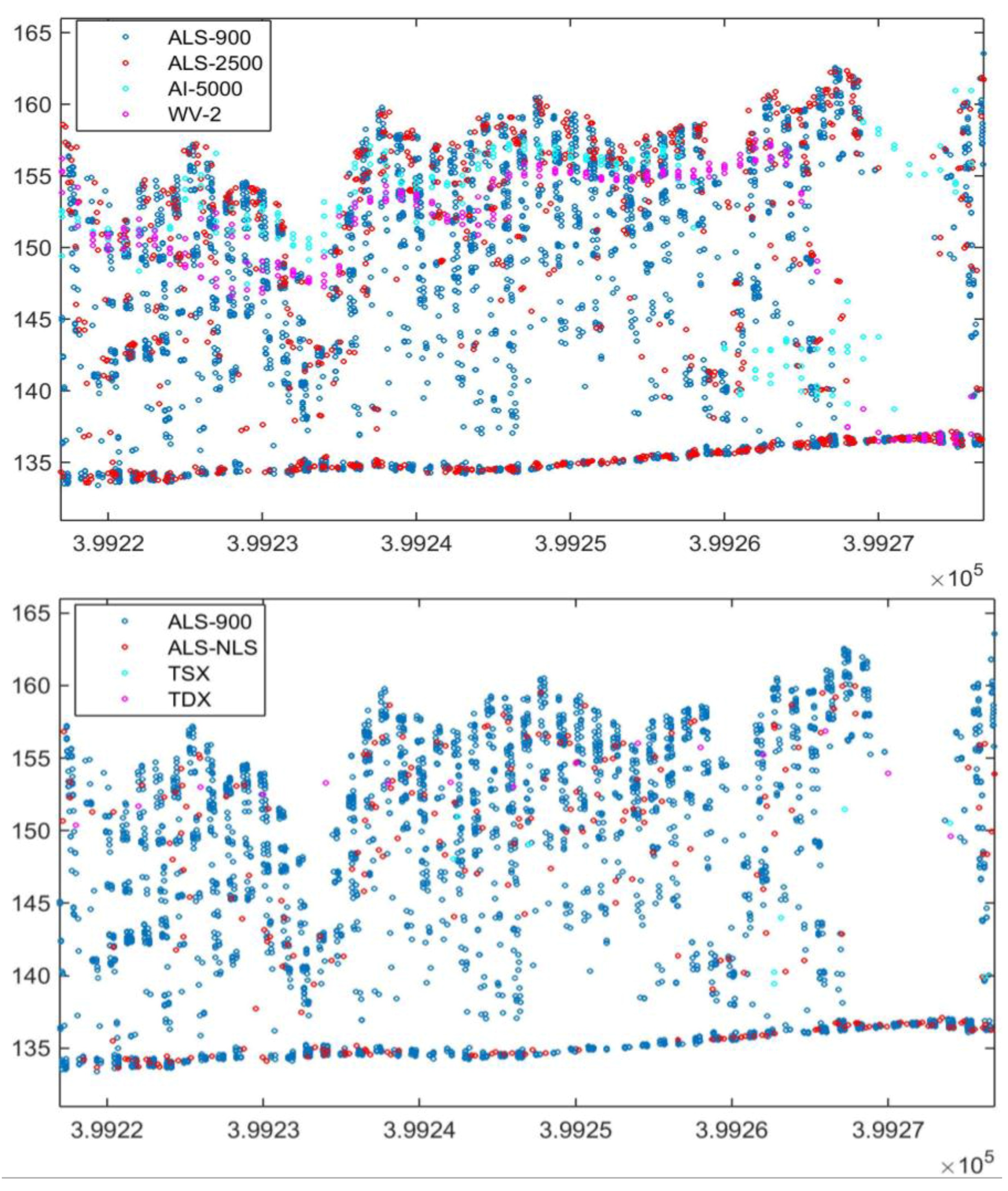
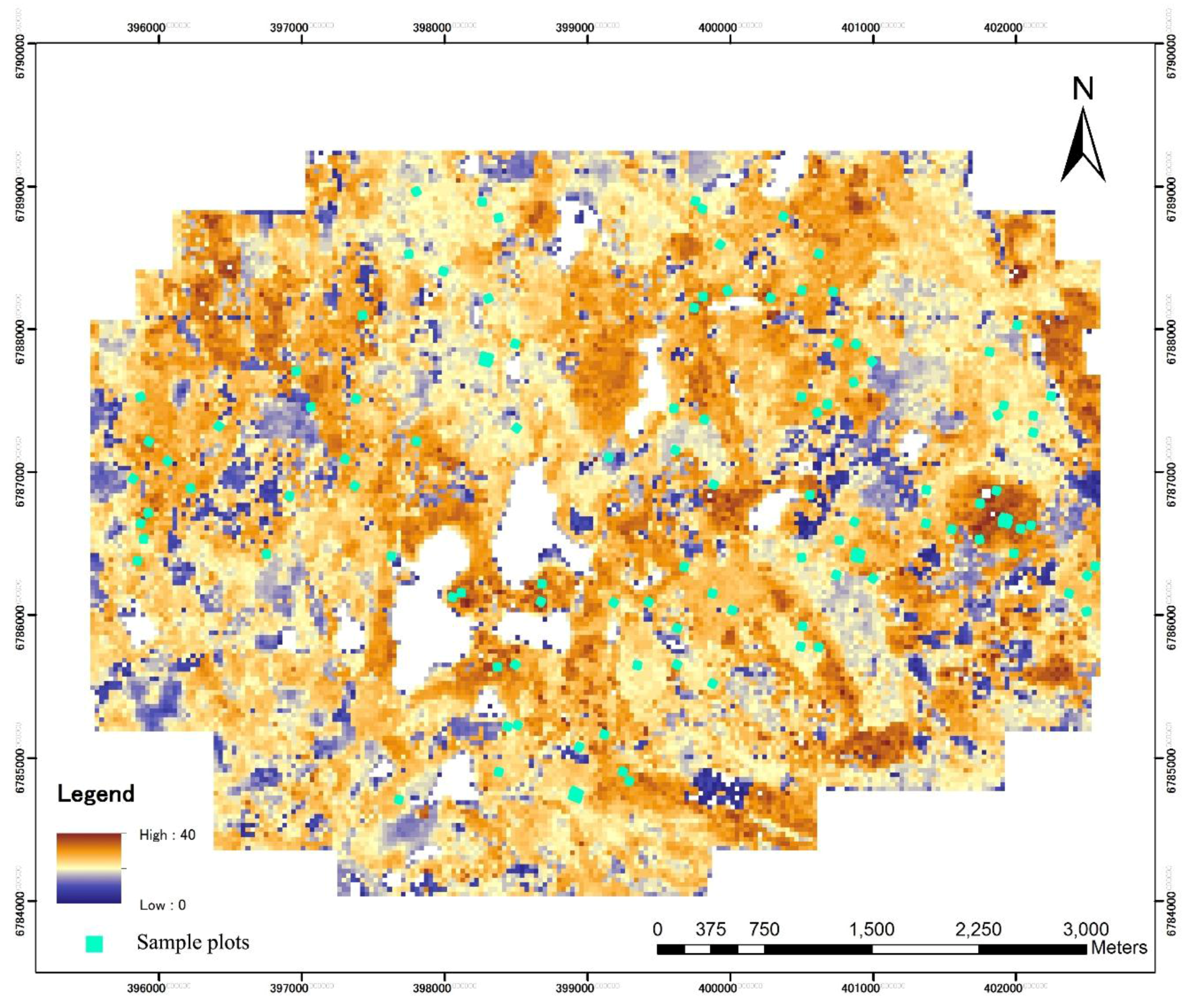
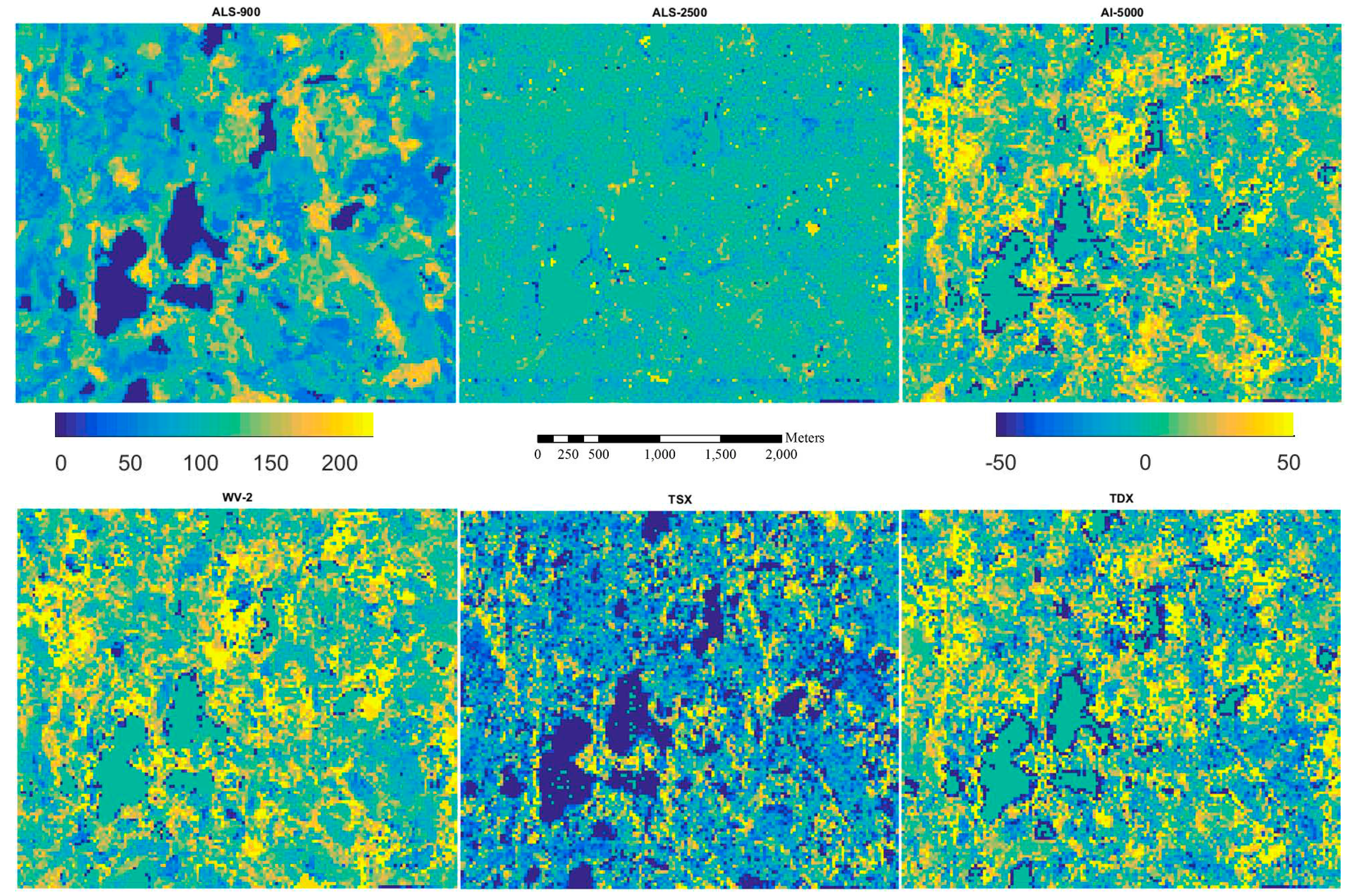
The combination of increasing spatial resolution and availability of 3D techniques has increased the ability to obtain vegetation information and monitor the changes. In principal, the image-based point clouds, either coming from optical images or SAR images, could be used for estimations of forest inventory attributes in a fashion analogous to ALS data, i.e., point cloud processing. However, the performance of point cloud produced by 3D techniques for the retrieval of forest inventory attributes has not been studied intensively. Most of the studies have been conducted in different test sites, and the differences in forest structure dominate the difference in the results. Therefore, there is a need to compare the capabilities of different point clouds generated in the same test site. In this study, we compared performance of 3D point cloud measured from very high resolution space-borne and airborne imagery and ALS point cloud for their capabilities in retrieval of forest inventory attributes in the area-based context. Remote sensing data used include TanDEM-X SAR Interferometry, TerraSAR-X SAR Data, WorldView-2 images, aerial images and ALS from different altitudes. The performance of 3D data was evaluated with 91 sample plots of size 32 m × 32 m and 16 m × 16 m in Evo, southern Finland.

2. Study Area and Materials

2.1. Test Site

The 5 km × 5 km study area, located in Evo, southern Finland (61.19°N, 25.11°E), belongs to the southern Boreal Forest Zone. It contains approximately 2000 ha of managed boreal forest, having an average stand size of slightly less than 1 ha. The area comprises of broad mixture of forest stands, varying from natural to intensively managed forests. The elevation of the area varies from 125 m to 185 m above sea level. Scots pine (Pinus sylvestris) and Norway spruce (Picea abies) are the dominant tree species in the study area and contribute 40% and 35% of the total volume, respectively, whereas the share of deciduous trees is 24% of the total volume.

2.2. Field Data

Field measurements were undertaken in summer 2014. The sampling of the field plots (32 m × 32 m, 1024 m²) was based on ALS data. First, a grid (32 m × 32 m) was placed over the area and ALS metrics describing forest height and density were calculated for each grid cell. The derived ALS metrics were mean height of vegetation calculated from the CHM and vegetation density at a height of 2 meters. Altogether, 120 sample plots were then selected with varying canopy heights and densities. However, only 91 sample plots were realized in the field (Figure 1). Rectangle plots of 32 m × 32 m were further divided into 4 plots of 16 m × 16 m in size which is the resolution used in forest mapping inventories collecting forest resource information for operational forest management and planning in Finland. Sample plot locations were determined using the geographic coordinates of the plot center and four corners. Plot center positions were measured using a total station (Trimble 5602), which was oriented to local coordinate system using ground control points measured with VRS-GNSS (Trimble R8) on open areas close to the plot.

Before field measurements, terrestrial laser scanning (TLS) measurements were carried out and tree maps were created based on TLS data. These tree maps were used to locate the trees in the field. Tree maps were checked during field measurements: missing trees were added to the maps and extra trees were deleted. Plot position was further adjusted manually against ALS data. In this procedure, the locations of all trees on the tree map were used to help find the true location of the plot with respect to the ALS point cloud. The plot was shifted and rotated so that the tree locations within the map properly aligned with the point cloud.

Figure 1. Study area and the location of sample plots. Background image is a canopy height model created from ALS data.

Figure 1. Study area and the location of sample plots. Background image is a canopy height model created from ALS data.

From the sample plots, all trees having a DBH exceeding 5 cm were tallied with steel calipers from two directions perpendicular to each other and a mean was taken as the value for DBH. Tree height was measured using an electronic hypsometer from all the trees as well. Height measurement accuracy is expected to be approximately 0.5 m. Lower limit of living crown and species were also recorded. The tree volumes and biomass were calculated using the standard Finnish models [33,34] with tree species, DBH, and height as inputs. The forest inventory attributes, i.e., basal-area weighted mean height (H_g), basal-area weighted mean DBH (D_g), basal area (G), volume (VOL) and total above ground biomass (AGB), for sample plots were obtained by averaging or summing the tree data. In this study, 32 m × 32 m plots are used as primary plots for developing prediction model and evaluating the accuracy. Additionally, the same procedure was also applied to 16 m × 16 m plots and results were compared with those of 32 m × 32 m plots to investigate how plot size affect the results. Only one of four neighboring subplots was selected to maintain independency of the sample plots in 16 m × 16 m case. The descriptive statistics of 32 m × 32 m and 16 m × 16 m plots are summarized in Table 1.

Table 1. The descriptive statistics of sample plots. (a) 91 sample plots of 32 m × 32 m, (b) 364 sample plots of 16 m × 16 m.

	Minimum	Maximum	Mean	Standard Deviation
(a) 91 sample plots of 32 m × 32 m
Hg (m)	10.02	31.09	21.09	4.41
Dg (cm)	13.92	46.42	25.78	7.50
G (m2/ha)	6.60	43.17	26.79	7.83
VOL (m3/ha)	34.46	518.39	270.14	110.04
AGB (Mg/ha)	19.06	230.63	134.49	48.33
Plot density (trees/ha)	342	3057	940	554
(b) 364 sample plots of 16 m × 16 m
Hg (m)	7.59	33.23	21.02	4.54
Dg (cm)	10.35	52.95	25.72	7.89
G (m2/ha)	3.67	57.26	26.79	9.17
VOL (m3/ha)	21.25	786.08	270.14	123.83
AGB (Mg/ha)	12.30	326.37	134.49	54.80
Plot density (trees/ha)	195	3242	940	596

Table 1. The descriptive statistics of sample plots. (a) 91 sample plots of 32 m × 32 m, (b) 364 sample plots of 16 m × 16 m.

	Minimum	Maximum	Mean	Standard Deviation
(a) 91 sample plots of 32 m × 32 m
Hg (m)	10.02	31.09	21.09	4.41
Dg (cm)	13.92	46.42	25.78	7.50
G (m2/ha)	6.60	43.17	26.79	7.83
VOL (m3/ha)	34.46	518.39	270.14	110.04
AGB (Mg/ha)	19.06	230.63	134.49	48.33
Plot density (trees/ha)	342	3057	940	554
(b) 364 sample plots of 16 m × 16 m
Hg (m)	7.59	33.23	21.02	4.54
Dg (cm)	10.35	52.95	25.72	7.89
G (m2/ha)	3.67	57.26	26.79	9.17
VOL (m3/ha)	21.25	786.08	270.14	123.83
AGB (Mg/ha)	12.30	326.37	134.49	54.80
Plot density (trees/ha)	195	3242	940	596

2.3. Remote Sensing Data and Preprocessing into Point Clouds

2.3.1. Airborne Laser Scanning Data

Airborne laser scanning data was acquired on 5 September 2014, using a Leica ALS70-HA SN7202 system (Leica Geosystems AG, Heerbrugg, Switzerland) operating at a pulse rate of 240 kHz. The data were collected from an altitude of 900 m above sea level at a speed of 150 knots, resulting in an average pulse density of approximately 6 pulses per m² and a footprint size of 13.5 cm in diameter (beam divergence of 0.15 mrad at 1/e point). The system was configured to record up to five echoes per pulse, i.e., first or only, last and 1 to 3 intermediates. The data are hereafter referred to as ALS-900.

The area was also covered by two surveys from 2500 m altitude above sea level: one on 22 May 2014 (three flightlines covered most part of the area) and other on 8 September 2014 (one flightline covered small part of the area). In both cases, data were collected using a Leica ALS70-HA SN7202 system operating at a pulse rate of 105 kHz and resulting in a pulse density of 0.7 pulses/m² in average and a footprint size of 37.5 cm in diameter. The system was configured to record up to five echoes per pulse, i.e., first or only, last and intermediates. The data are hereafter referred to as ALS-2500.

Both ALS data were geo-referenced in the ETRS-TM35FIN coordinate system and calibrated for heading, pitch and roll by the data provider. Afterwards, the ALS data were first classified into ground or non-ground points using the standard approach of the TerraScan based on the method explained by Axelson [35]. A DTM was then created using classified ground points. Laser heights above ground (normalized height or canopy height) were calculated by subtracting the ground elevation from the corresponding laser height measurements.

2.3.2. Open ALS Data

In addition to the aforementioned ALS data, the National Land Survey of Finland (NLS) has conducted ALS campaigns since 2003, with the goal of scanning entire country in order to generate an accurate DTM. These ALS datasets (hereafter referred to as ALS-NLS) were also included in the comparison because they are publicly available and thus are highly interesting for many end-users. The study area was surveyed partly with a Leica ALS50 scanner and partly with an Optech scanner in 2012. The flying altitude was 2200 m and 1830 m above sea level, respectively, and the pulse density was around 0.8 pulses per square meter in both surveys. The data were geo-referenced, calibrated and classified by data provider. Table 2 summarizes the technical specifications of ALS surveys.

Table 2. Technical specifications for airborne laser scanning (ALS) data used in this study.

	ALS from 900 m Altitude (ALS-900)	ALS from 2500 m Altitude (ALS-2500)	ALS from NLS Open Data (ALS-NLS)
Date	5 September 2014	22 May 2014/8 September 2014	7 May 2012/13 May 2012
Scanner	Leica ALS70-HA SN7202	Leica ALS70-HA SN7202	Optech ALTM GEMINI/Leica ALS50
Altitude (m)	900	2500	1830/2200
Pulse density (pulses/m2)	6	0.7/0.7	0.8/0.8
Pulse rate (KHz)	240	105
Accuracy in XY (cm)	10	15	30/20
Accuracy in Z (cm)	8	8	15/10

Table 2. Technical specifications for airborne laser scanning (ALS) data used in this study.

	ALS from 900 m Altitude (ALS-900)	ALS from 2500 m Altitude (ALS-2500)	ALS from NLS Open Data (ALS-NLS)
Date	5 September 2014	22 May 2014/8 September 2014	7 May 2012/13 May 2012
Scanner	Leica ALS70-HA SN7202	Leica ALS70-HA SN7202	Optech ALTM GEMINI/Leica ALS50
Altitude (m)	900	2500	1830/2200
Pulse density (pulses/m2)	6	0.7/0.7	0.8/0.8
Pulse rate (KHz)	240	105
Accuracy in XY (cm)	10	15	30/20
Accuracy in Z (cm)	8	8	15/10

2.3.3. Aerial Images

The aerial images were acquired in May 2014 at 5 km altitude (refereed as to AI-5000). The imaging sensor used was a Z/I Imaging Digital Mapping Camera (DMC) [36] with a stereoscopic forward overlap of 80% and side overlap of 64%. The area was covered by 24 images in total. Images were taken from two separate flight lines of 12 images each. The ground-sample distance (GSD) was approximately 0.5 m. Specific data characteristics are provided in Table 3. The image orientation was completed using BAE Systems Socet Set software with direct geo-referencing data as an initial solution for bundle adjustment. Socet Set is a professional digital workstation, including tools for precision photogrammetry and multisensoral triangulation to digital mapping. Forty ground control points (GCP) were digitized from the images and reference data. Three radial distortion parameters were solved in on-the-job calibration. The RMSEs of the orientation were 26.6 cm, 40.0 cm and 1.19 m in the X, Y and Z directions, respectively. Socet Set was also the main software package used in the extraction of 3D information from the stereo aerial and satellite images. The automatic matching of image pairs in the calculation of 3D surface points was carried out using the NGATE (Next Generation Automatic Terrain Extraction) module of the Socet Set workstation. NGATE combines area-based and feature-based methods to calculate similarity measurements on the basis of a cross-correlation approach. Basically, the process is fully automatic and the user can guide the process by changing a few parameters related to the matching algorithm. The main parameters are used to control the number and accuracy of the resulting 3D points (successfully matched points between images). The matching strategy used with the aerial images was tuned for forestry applications. For example, the image correlation window size was 11 × 11 pixels for all image pyramid levels, sudden surface model steepness was enabled in the lowest five pyramid levels, and edge matching search distance was increased in the lowest six pyramid levels. The detailed process regarding the 3D extraction is described by Nurminen et al. [13].

2.3.4. WorldView-2 Satellite Imagery

Optical satellite images used were acquired from WorldView-2 satellite (WV-2) because of its possibility to obtain in-track stereo pairs with very high spatial resolution. WV-2 is a commercial optical satellite owned and operated by DigitalGlobe. WV-2 was launched in October 2009, and it provides panchromatic images with the GSD of 0.50 m at the nadir, which corresponds to the GSD of the aerial images with flying altitude of 5 km in this study. WV-2 also provides multispectral images; however, with slightly degraded GSD. A cloud-free image pair was acquired on 11 July 2014, which covered the entire test area. The basic information of the WV-2 image pair is the following: in-track basic stereo panchromatic product, GSD of approximate 0.5 m, acquired at around midday local time, convergence angle of 13.6°, off-nadir angles of 6.8° and 13.6° for the first and the second image respectively (Table 3). The geo-positioning accuracy of WV-2 image pair was good; however, there was a clear need to refine geo-positioning using GCPs. Socet Set was used and 10 GCPs were digitized from the images. The resulting RMSE of the triangulation solution was 0.3 meters, which is well below the pixel size. Then 3D points were generated using NGATE module of the Socet Set workstation similarly to the aerial image case. In the matching of WorldView-2 stereo images, one of the NGATE default strategy was used after visual comparison of couple of default strategies. In this case, the urban canyon strategy appeared to perform the best among other strategies. However, the differences between the default matching strategies were marginal.

Table 3. Characteristics of aerial images (AI-5000) and WorldView-2 (WV-2).

	Acquisition Date	Flight Altitude (km)	Overlap	Ground Sampling Distance (m)	Images or Image Pairs	Convergence Angle/off Nadir Angle (degree)
AI-5000	22 May 2014	5	80% forward/64% side	0.5	24 in two strips
WV-2	11 July 2014	770	Along track	0.5	1	13.6/(6.8, 13.6)

Table 3. Characteristics of aerial images (AI-5000) and WorldView-2 (WV-2).

	Acquisition Date	Flight Altitude (km)	Overlap	Ground Sampling Distance (m)	Images or Image Pairs	Convergence Angle/off Nadir Angle (degree)
AI-5000	22 May 2014	5	80% forward/64% side	0.5	24 in two strips
WV-2	11 July 2014	770	Along track	0.5	1	13.6/(6.8, 13.6)

2.3.5. TerraSAR-X Satellite Data

TerraSAR-X (TSX) satellite data were used in the stereo-radargrammetric part of the study. TSX is a German satellite, launched in 2007, and is capable of acquiring SAR images with a spatial resolution of about one meter. TSX operates at the X-band microwave region having the wavelength of 3.1 cm. Altogether six TSX images were available from summer 2014, covering the test area and were acquired in a time period of 10 days. Weather conditions in that time were stable. All TSX images were Multi-look Ground Range Detected (MGD) products, in HH polarization and in the Spotlight imaging mode. The set of six TSX images forms six stereo pairs suitable for 3D radargrammetric processing, the TSX pairs being: D1 + D2, D1 + D3, D2 + D3, A1 +A2, A1 + A3, and A2 + A3. Based on the visual inspection of TSX data against existing map data (aerial orthoimage and ALS based elevation model), we can conclude that the geo-positional accuracy of TSX data was in the order of 1–2 meters and comparable to the TSX image pixel size; therefore, there was no need to refine the geo-positioning parameters included in the orbit data of the original images. The TSX images used in the study are listed in Table 4.

Table 4. TerraSAR-X (TSX) and TanDEM-X (TDX) SAR image pairs used in the study.

Source	ID	Date	Incidence Angle (°)	Time (UTC)	Orbit	Weather(°C)	Resolution	Notes
TSX	D1	9 July 2014	26	4:57	Desc./right	19		Clear
	D2	4 July 2014	36	4:48	Desc./right	14		Clear
	D3	29 June 2014	44	4:40	Desc./right	14		Rain showers
	A1	9 July 2014	30	15:45	Asc./right	27		Clear
	A2	3 July 2014	40	15:54	Asc./right	18		Clear
	A3	8 July 2014	47	16:03	Asc./right	25		Clear, possibly rain showers
TDX		5 June 2014	48	16:03	Asc.	26	2.4 m in range/3.3 m in azimuth	Clear

Table 4. TerraSAR-X (TSX) and TanDEM-X (TDX) SAR image pairs used in the study.

Source	ID	Date	Incidence Angle (°)	Time (UTC)	Orbit	Weather(°C)	Resolution	Notes
TSX	D1	9 July 2014	26	4:57	Desc./right	19		Clear
	D2	4 July 2014	36	4:48	Desc./right	14		Clear
	D3	29 June 2014	44	4:40	Desc./right	14		Rain showers
	A1	9 July 2014	30	15:45	Asc./right	27		Clear
	A2	3 July 2014	40	15:54	Asc./right	18		Clear
	A3	8 July 2014	47	16:03	Asc./right	25		Clear, possibly rain showers
TDX		5 June 2014	48	16:03	Asc.	26	2.4 m in range/3.3 m in azimuth	Clear

The NGATE module of the Socet Set software was also used in the image matching and 3D point calculation. The acceptance threshold of the cross-correlation value in the matching phase can be changed. When the threshold value gets lower, more 3D points will exist in the results. However, at the same time the number of incorrect matches increases. In general, there is no clear rule for setting the threshold value, and it depends heavily on the images used in the process (the range of cross-correlation values is 0–100). In optical images acquired nearly simultaneously the value can be as high as 90, and on the other hand for SAR images about 50–70. The result of the NGATE process is a set of 3D points, i.e., successfully matched points and their 3D object coordinates, which were exported for further processing. The more detailed information is given by Karjalainen et al. [23].

2.3.6. TanDEM-X SAR Interferometry Data

In the InSAR part of the study, TanDEM-X (TDX) data were used. TDX system consists of two identical satellites, TerraSAR-X and TanDEM-X, which can be used in a bistatic imaging mode (one being a transmitting system, and both being in the receiving mode). As the TDX data acquisition is simultaneous, the system is particularly suitable for creating DSM. The basic information about the TDX image pair used in present study is given in Table 4. Unfortunately, there was only one TDX data acquisition available in June 2014. TDX acquisition was made in the Stripmap imaging mode, which corresponds to the resolution of 2.4 m in ground range and 3.3 m in azimuth direction. The interferometric baseline of this pair was 190 m, which equals to the height-of-ambiguity of 45 m. The image was acquired using HH polarization.

The interferometric data was processed using the SARscape 5.0 software package. The original data was in co-registered single-look complex (CoSSC) format. First, a multilooked (2 by 2 pixels) interferogram was generated and flat earth phase was removed from the interferogram. Then, the interferogram was filtered using the Goldstein filter with a window of 10 by 10 pixels, and phase unwrapping was carried out using the Delaunay Minimum Cost Flow algorithm with a coherence threshold of 0.25, which was also the coherence threshold used in the output product. The output was a surface point cloud resampled to 4 m ground pixel size. No interpolation of height values was applied. Finally, height calibration was done using nine reference areas, which were located in different parts of the study area. The reference areas (200–500 m²) were open areas (e.g., fields, clear cuts) and the average height of each area was measured from ALS data. The average ALS height and average InSAR height were compared to get the absolute elevation level correctly into the InSAR elevation model. The detailed process regarding the InSAR 3D extraction is described by Karila et al. [27].

3. Methods

For prediction of forest inventory attributes, i.e., H_g, D_g, G, VOL and AGB, the same method and procedure were applied using point clouds either produced from RS data or collected from ALS. The workflow is shown in Figure 2. The more detailed description of each step is given in the following sections. In addition, we also compare the point clouds produced from stereo images with ALS point cloud (ALS-900) and evaluate the feature importance for their potential power in predicting the forest attributes. The effects of the plot size on the prediction are also investigated.

3.1. Data Co-Registration

Besides the geometric correction before 3D point production, image-based point clouds were also visually inspected with respect to ALS point cloud collected from 900 m altitude for the possible horizontal and vertical displacements. If such displacement existed, the difference was measured and corrected accordingly. Then all datasets were normalized to heights above ground using a DTM derived from ALS-900 data by subtracting the ground elevation from height at the corresponding location of the 3D points.

3.2. Plot Feature Derivation

From each point cloud data, the various height distribution related features were calculated and used as predictors in the regression for developing prediction models because they have been proved to be effective in predicting forest attributes [4,37,38,39]. Most of the features were calculated from normalized points above the 2 m threshold. Firstly, some descriptive statistics were computed from all returns or points. These included maximum height (Hmax), mean height calculated as the arithmetic mean of heights (Hmean), mode of heights (Hmode), standard deviation of the heights (Hstd), coefficient of variation (Hcv), penetration rate (PR) as a ratio of ground returns to total number of returns, canopy volume (Vc) as the multiplication of mean height and ratio of the number of returns above 2 m to the total number of returns. Secondly, the various percentiles were calculated from 10% to 90% of canopy height distribution with a 10% increment (HP₁₀–HP₉₀). Finally, each point cloud was divided into 10 equal intervals of height, starting at the canopy bottom (2 m) and ending at the top and then canopy cover density was computed as proportion of points in each interval to total number of points (CC₁–CC₁₀). Detailed definitions and calculations are given in Table 5.

Figure 2. Flowchart of the method and procedure for prediction of forest attribute using point cloud.

Figure 2. Flowchart of the method and procedure for prediction of forest attribute using point cloud.

Table 5. Plot features derived from normalized point data.

Feature	Definition
Hmax	Maximum of the normalized heights of all points
Hmean	Arithmetic mean of normalized height of all points above 2 m threshold
Hmod	Mode of normalized height of all points above 2 m threshold
Hstd	Standard deviation of normalized height of all points above 2 m threshold
Hcv	coefficient of variation calculated as Hstd/Hmean
PR	Nh<= 2/Ntotal, where Ntotal is the number of all points, and Nh<= 2 the number of points below and equal to 2 m.
Vc	Canopy volume calculated as Hmean*(1-PR)
HP10–HP90	10% to 90% percentiles of normalized height of all points above 2 m threshold with a 10% increment
CC1–CC10	CCi = Ni/Ntotal, where i = 1 to 10, Ni is the number of points within ith layer when tree height was divided into 10 intervals starting from 2 m, Ntotal is the number of all points.

Table 5. Plot features derived from normalized point data.

Feature	Definition
Hmax	Maximum of the normalized heights of all points
Hmean	Arithmetic mean of normalized height of all points above 2 m threshold
Hmod	Mode of normalized height of all points above 2 m threshold
Hstd	Standard deviation of normalized height of all points above 2 m threshold
Hcv	coefficient of variation calculated as Hstd/Hmean
PR	Nh<= 2/Ntotal, where Ntotal is the number of all points, and Nh<= 2 the number of points below and equal to 2 m.
Vc	Canopy volume calculated as Hmean*(1-PR)
HP10–HP90	10% to 90% percentiles of normalized height of all points above 2 m threshold with a 10% increment
CC1–CC10	CCi = Ni/Ntotal, where i = 1 to 10, Ni is the number of points within ith layer when tree height was divided into 10 intervals starting from 2 m, Ntotal is the number of all points.

3.3. Prediction of Forest Inventory Attributes

In this study, forest attributes were predicted based on 3D data-derived features and field measurements using area-based approach and random forest (RF) technique [2,12,40]. Typically, in area-based methods, percentiles and other height related features are used to predict forest inventory attributes at resolution varying from typically 100 m² to 1000 m², using parametric or nonparametric estimation techniques. In this study, point clouds from plot areas were first extracted from the data and plot features were derived individually per plot from the normalized height as described in previous section. Then, prediction models were developed based on these features and field measured forest inventory attributes using RF technique [41]. Finally, forest attributes were estimated based on the developed models and plot features derived for the areas.

Random forest is a nonparametric regression method in which the RF prediction is obtained by aggregating regression trees, each constructed using an independently drawn bootstrap replica of the training data, and choosing splits of the regression trees from subsets of the available features, randomly chosen at each node. We used RF to construct the prediction models because it works well when many features are available and no variable selection procedures are needed. Furthermore, RF makes no assumption on the distribution of the data. In the regression process with RF, plot features were used as predictors and inventory attribute as response variable. Prediction models were then developed by creating an ensemble of regression trees that each was built by a random selection of two thirds of plots. Thus, remaining one-third of the plots (referred as to out-of-bag samples) were used for testing. The idea behind this is that separate testing data is not necessary and this is one of the merits of the RF. Another advantage of the RF is that the algorithm provides a measure for feature importance assessment. Feature importance measures produced by the RF algorithm provided an insight into which object features were relatively more important for estimation of any given forest attribute. In this study, we carried out RF in MATLAB with parameter settings as follows: 200 regression trees were created; 8 predictors were randomly selected at each node for the best splitting; minimum size of the leaf nodes was set to be 2. We compute predictions for each tree on its out-of-bag observations and then average these predictions over the entire ensemble for each observation. This way, we can compare the predicted out-of-bag response with the true value for a realistic estimation of prediction error.

3.4. Evaluation of Accuracy

To evaluate the performance of RS data source for predicting forest inventory attributes, namely H_g, D_g, G, VOL and AGB, the correlation coefficient (R) between predicted and reference values was calculated as a measure for the goodness of fit of the prediction model. Bias and RMSE between the predicted and observed values were also computed as a measure for error estimates and were calculated as follows:

$$bias=\frac{{\displaystyle \sum _{i=1}^n({\widehat{X}}_i-X_i)}}{n}$$

(1)

$$RMSE=\sqrt{\frac{{\displaystyle \sum _{i=1}^n{({\widehat{X}}_i-X_i)}^2}}{n}}$$

(2)

where n is the number of plots, ${\hat{X}}_i$the value estimated from RS data for plot i, and Xi the observed value for plot i. The relative bias and RMSE were calculated according to the sampled mean $\overline{X}$of the variable in question as follows:

$$bias(\%)=\frac{bias}{\overline{X}}\times 100$$

(3)

$$RMSE(\%)=\frac{RMSE}{\overline{X}}\times 100$$

(4)

4. Results and Discussion

4.1. Image-based Point Cloud versus ALS Point Cloud

Table 6 shows point density statistics of ALS point cloud and image-based point clouds based on 91 sample plots. In general, image-based point density decreased as image spatial resolution decreased. For ALS data, point density decreased as flight altitude increased. Thus we have a dataset having point density varied from 0.05 pts/m² to 12 pts/m² in average.

Table 6. Point density (points/m²) statistics of remote sensing (RS) 3D data based on 91 sample plots.

	ALS-900	ALS-2500	ALS-NLS	AI-5000	WV-2	TSX	TDX
Minimum	7.64	0.82	0.72	0.76	0.55	0.03	0.00
Maximum	20.34	1.43	7.67	1.00	1.01	0.13	0.06
Mean	11.96	1.18	2.67	0.96	0.90	0.06	0.05

Table 6. Point density (points/m²) statistics of remote sensing (RS) 3D data based on 91 sample plots.

	ALS-900	ALS-2500	ALS-NLS	AI-5000	WV-2	TSX	TDX
Minimum	7.64	0.82	0.72	0.76	0.55	0.03	0.00
Maximum	20.34	1.43	7.67	1.00	1.01	0.13	0.06
Mean	11.96	1.18	2.67	0.96	0.90	0.06	0.05

Compared to laser scanning, the main limitations of image-based 3D techniques are the impossibility of acquiring under-canopy information and the smoothing effect of the canopy surface (Figure 3). This trend was also verified by the difference of features between ALS and image-based point clouds. For example, when compared with ALS-900 data, Hmax decreased in average by 0.6 m (ALS-2500), 1.9 m (AI-5000), 3.3 m (WV-2), 3.7 m (TSX) and 7.5 m (TDX), respectively. Hmean increased in average by 0.7 m (ALS-2500), 3.2 m (AI-5000), 1.6 m (WV-2), and 0.1 m (TDX), respectively, while decreased by 0.8 m for TSX. Most of points were distributed in vertical direction about 1 m higher in WV-2 and about 1 m, 10 m and 6 m lower in AI-5000, TSX and TDX point clouds than in ALS-900 data.

Figure 3. Profiles of 60 m long and 4 m wide section of various data.

Figure 3. Profiles of 60 m long and 4 m wide section of various data.

4.2. Accuracy of Plot Attribute Estimation

Table 7 shows a summary of the accuracy statistics for estimation of H_g, D_g, G, VOL and AGB using area-based approach and RF regression technique. It can be seen from table that relative RMSE varied between 4.6% and 13.4% for H_g, 11.7% and 20.6% for D_g, 14.8% and 25.8% for G, 15.9% and 31.2% for VOL and 14.3% and 27.5% for AGB depending on the RS data used. As expected, ALS data produced most accurate estimates for all forest inventory attributes. Changes in point density or flight altitude of ALS data has little effect on the estimation when area-based method was used for prediction. Aerial image point cloud performed slightly worse than ALS data with one to three percentage points increase in relative RMSEs, but not significantly different from the result obtained from ALS data based on Kruskal-Wallis test at 5% significant level. WV-2 point cloud worked well surpassing the aerial image and reaching the accuracy level of higher altitude ALS data (ALS-2500, ALS-NLS) for VOL and AGB estimates. Higher relative RMSEs were obtained from both TSX and TDX point clouds. When two radar data were compared, TDX achieved a better accuracy (lower RMSE) than TSX since interferometry typically creates higher quality data than radargrammetry does, but the availability of the data is more limited. Kruskal–Wallis test, however, indicated that there is no significant difference between the estimates from TDX and TSX data. A summary of significant tests on estimates of forest attributes between different datasets is given in supplementary Table S1. Relative RMSEs are also graphically presented in Figure 4. Biases for all the data sources and for all attribute estimates were small which suggested that prediction models performed well for calibrating the systematic errors.

Table 7. Accuracy assessments of forest attribute estimation from 3D point clouds using area-based approach.

	Bias	Bias (%)	RMSE	RMSE (%)	R
ALS-900
Hg (m)	0.02	0.11	1.12	5.30	0.97
Dg (cm)	0.08	0.33	3.28	12.74	0.90
G (m2/ha)	0.15	0.57	3.95	14.75	0.86
Vol (m3/ha)	2.38	0.88	42.99	15.91	0.92
AGB (Mg/ha)	0.77	0.57	19.18	14.26	0.92
ALS-2500
Hg (m)	0.05	0.23	0.97	4.61	0.98
Dg (cm)	0.07	0.28	3.03	11.74	0.91
G (m2/ha)	0.13	0.48	4.26	15.91	0.84
Vol (m3/ha)	0.64	0.24	43.52	16.11	0.92
AGB (Mg/ha)	−0.07	−0.05	21.29	15.83	0.90
ALS-NLS
Hg (m)	0.05	0.22	1.09	5.17	0.97
Dg (cm)	0.01	0.04	3.05	11.82	0.91
G (m2/ha)	0.09	0.33	4.23	15.80	0.84
Vol (m3/ha)	1.41	0.52	45.16	16.72	0.91
AGB (Mg/ha)	0.21	0.16	21.47	15.96	0.90
AI-5000
Hg (m)	0.00	0.00	1.46	6.90	0.94
Dg (cm)	0.11	0.42	3.34	12.94	0.89
G (m2/ha)	0.12	0.43	4.89	18.24	0.78
Vol (m3/ha)	1.64	0.61	52.34	19.37	0.88
AGB (Mg/ha)	−0.11	−0.08	24.01	17.85	0.87
WV-2
Hg (m)	−0.01	−0.03	1.40	6.63	0.95
Dg (cm)	−0.01	−0.04	3.44	13.33	0.89
G (m2/ha)	0.03	0.12	4.32	16.11	0.83
Vol (m3/ha)	1.45	0.54	42.95	15.90	0.92
AGB (Mg/ha)	0.31	0.23	21.79	16.20	0.89
TSX
Hg (m)	−0.17	−0.83	2.83	13.40	0.77
Dg (cm)	−0.14	−0.53	5.32	20.62	0.70
G (m2/ha)	0.03	0.12	6.91	25.79	0.49
Vol (m3/ha)	0.59	0.22	84.19	31.17	0.64
AGB (Mg/ha)	−0.21	−0.16	36.97	27.49	0.64
TDX
Hg (m)	0.00	−0.02	2.01	9.53	0.89
Dg (cm)	−0.02	−0.07	4.95	19.20	0.75
G (m2/ha)	−0.15	−0.58	5.58	20.85	0.70
Vol (m3/ha)	−0.29	−0.11	59.32	21.96	0.84
AGB (Mg/ha)	0.20	0.15	27.83	20.69	0.82

Table 7. Accuracy assessments of forest attribute estimation from 3D point clouds using area-based approach.

	Bias	Bias (%)	RMSE	RMSE (%)	R
ALS-900
Hg (m)	0.02	0.11	1.12	5.30	0.97
Dg (cm)	0.08	0.33	3.28	12.74	0.90
G (m2/ha)	0.15	0.57	3.95	14.75	0.86
Vol (m3/ha)	2.38	0.88	42.99	15.91	0.92
AGB (Mg/ha)	0.77	0.57	19.18	14.26	0.92
ALS-2500
Hg (m)	0.05	0.23	0.97	4.61	0.98
Dg (cm)	0.07	0.28	3.03	11.74	0.91
G (m2/ha)	0.13	0.48	4.26	15.91	0.84
Vol (m3/ha)	0.64	0.24	43.52	16.11	0.92
AGB (Mg/ha)	−0.07	−0.05	21.29	15.83	0.90
ALS-NLS
Hg (m)	0.05	0.22	1.09	5.17	0.97
Dg (cm)	0.01	0.04	3.05	11.82	0.91
G (m2/ha)	0.09	0.33	4.23	15.80	0.84
Vol (m3/ha)	1.41	0.52	45.16	16.72	0.91
AGB (Mg/ha)	0.21	0.16	21.47	15.96	0.90
AI-5000
Hg (m)	0.00	0.00	1.46	6.90	0.94
Dg (cm)	0.11	0.42	3.34	12.94	0.89
G (m2/ha)	0.12	0.43	4.89	18.24	0.78
Vol (m3/ha)	1.64	0.61	52.34	19.37	0.88
AGB (Mg/ha)	−0.11	−0.08	24.01	17.85	0.87
WV-2
Hg (m)	−0.01	−0.03	1.40	6.63	0.95
Dg (cm)	−0.01	−0.04	3.44	13.33	0.89
G (m2/ha)	0.03	0.12	4.32	16.11	0.83
Vol (m3/ha)	1.45	0.54	42.95	15.90	0.92
AGB (Mg/ha)	0.31	0.23	21.79	16.20	0.89
TSX
Hg (m)	−0.17	−0.83	2.83	13.40	0.77
Dg (cm)	−0.14	−0.53	5.32	20.62	0.70
G (m2/ha)	0.03	0.12	6.91	25.79	0.49
Vol (m3/ha)	0.59	0.22	84.19	31.17	0.64
AGB (Mg/ha)	−0.21	−0.16	36.97	27.49	0.64
TDX
Hg (m)	0.00	−0.02	2.01	9.53	0.89
Dg (cm)	−0.02	−0.07	4.95	19.20	0.75
G (m2/ha)	−0.15	−0.58	5.58	20.85	0.70
Vol (m3/ha)	−0.29	−0.11	59.32	21.96	0.84
AGB (Mg/ha)	0.20	0.15	27.83	20.69	0.82

Figure 4. Relative root mean square errors (RMSE)s of forest attribute estimates from RS point clouds.

Figure 4. Relative root mean square errors (RMSE)s of forest attribute estimates from RS point clouds.

Figure 5, Figure 6, Figure 7, Figure 8 and Figure 9 show the inventory map from ALS-900 data and the difference maps between using ALS-900 and other point clouds except ALS-NLS data, because it is quite similar to the one using ALS-2500 data. From these figures, it can be seen that similar results were obtained for most parts of the area. However, in some particular forested areas, estimates differed considerably. When further investigations were performed on these forested areas, it was found that the image matching was problematic. For example, in a single story sparsely forested area, image matching was not accurate with AI-5000 and WV-2 images probably because it is difficult to correctly detect the matching points between images due to the high degree of variations in height. The problem in matching is that wrong height was given by AI-5000, whereas image matching was normally failed, i.e., no point was produced with WV-2 data. This is maybe one reason why WV-2 data performed better than AI-5000 data. It should be pointed out that TSX data has the tendency to overestimate the attributes of low biomass forests. There were also considerable amount of points created from TSX data over water area so the lakes are more visible on the difference maps between ALS-900 and TSX data.

Figure 5. Inventory map for H_g (m) from ALS-900 (first image) and the difference of inventory maps between ALS-900 and other RS data.

Figure 5. Inventory map for H_g (m) from ALS-900 (first image) and the difference of inventory maps between ALS-900 and other RS data.

Figure 6. Inventory map for D_g (cm) from ALS-900 (first image) and the difference of inventory maps between ALS-900 and other RS data.

Figure 6. Inventory map for D_g (cm) from ALS-900 (first image) and the difference of inventory maps between ALS-900 and other RS data.

Figure 7. Inventory map for G (m²/ha) from ALS-900 (first image) and the difference of inventory maps between ALS-900 and other RS data.

Figure 7. Inventory map for G (m²/ha) from ALS-900 (first image) and the difference of inventory maps between ALS-900 and other RS data.

Figure 8. Inventory map for Vol (m³/ha) from ALS-900 (first image) and the difference of inventory maps between ALS-900 and other RS data.

Figure 8. Inventory map for Vol (m³/ha) from ALS-900 (first image) and the difference of inventory maps between ALS-900 and other RS data.

Figure 9. Inventory map for AGB (Mg/ha) from ALS-900 (first image) and the difference of inventory maps between ALS-900 and other RS data.

Figure 9. Inventory map for AGB (Mg/ha) from ALS-900 (first image) and the difference of inventory maps between ALS-900 and other RS data.

The results in this study are in line with previous studies, for example, Järnstedt et al. [18] and Nurminen et al. [13] where ALS and aerial image (AI) point cloud are compared. Nurminen et al. [13] obtained similar estimation results from both ALS and AI point clouds for plot level attributes while Järnstedt et al. [18] reported a slightly better accuracy from ALS than AI data. In both studies, AI data were obtained from a lower altitude and with a better GSD. Bohlin et al. [17] achieved a relative RMSE of 8.8% for tree height, 13.1% for stem volume and 14.9% for basal area from AI data corresponding to the standard acquisition of the Swedish National Land Survey. In Vastaranta et al. [19], height, diameter, basal area, stem volume, and biomass were predicted with RMSE of 11.2%, 21.7%, 23.6%, 24.5%, and 23.7%, respectively, from AI data, whereas respective accuracies for the ALS-based predictions were 7.8%, 19.1%, 17.8%, 17.9%, and 17.5% using datasets similar to those used in Järnstedt et al. [18]. In Persson and Fransson [24], biomass at the stand level were estimated with 22.9% relative RMSE, while the height estimation showed 9.4% using TSX radargrammetry in a boreal forest. The better accuracy in their study is contributed to larger size, i.e., stand level estimates compared to plot size in this study. Karjalainen et al. [23] found that the forest stem volume could be predicted with 34.0% relative RMSE and the mean forest height with 14.0% using TSX radargrammetry data at plot level, which are slightly worse than those obtained in this study. In Karila et al. [27], the relative RMSE of 32% was obtained for stem volume, 20% for mean height, and 29% for basal area at plot level from TDX InSAR data, which were about 10 percentage points larger than the values archived in this study. The reason for larger RMSEs could be a smaller plot size used in their study. Rahlf et al. [32] reported relative RMSEs of 19% from ALS followed by 31% from AI data, 42% from TDX data, and 44% from TSX data for volume at plot level. Different prediction models and smaller plot size were used in their study. The differences in these results are most likely due to the differences in data resolution, prediction methods and prediction level. Forest conditions are also one factor that could influence the results. However, most of the studies were conducted in boreal forest.

It should be noted that DTM describing the ground elevation, such as derived from ALS data, must be available in order to use image-based point cloud in the retrieval of forest inventory attributes. The other challenge in the use of 3D techniques is image matching which has been well known to be quite challenging, in particular over forested area due to the factors, such as omissions, repetitive texture and multi-layered, shadows or moving objects [20,42]. In the present study, it was observed that matching strategy used was better suited to deciduous stands than to conifer stands. The density of the plot also influenced the success of image matching: plots with continuous canopy cover were much more accurately reconstructed than plots presenting local gaps between tree crowns. From visual inspection, it was found that plots with large estimation errors were young or sparse plots. The reason for this is probably the abrupt vertical changes in latter case, which were difficult to model accurately. Other image matching strategies may need to be explored to see how they work in such a case. In the image matching based approach the image resolution also impacts the level of detail of the DSMs, and the overlaps used in the data capture impact the resulting DSM quality; further studies on these topics are necessary in order to optimize the performance of the photogrammetric method.

Regardless of these limitations, 3D techniques still provide superior capabilities for accurately measuring vegetation structure compared to 2D data, especially radar data that have been somewhat deficient, as the amplitude of the radar signal tends to saturate at certain level of biomass, and higher biomasses cannot be measured accurately [43,44]. In this study, there are no apparent sign of saturation in predicting high biomass as it normally occurred with optical and radar images. This indicates that radar image-based point cloud has great potentials in large area mapping and in the monitoring of changes in the forest structure because of its more frequent coverage and its ability to acquire images through clouds compared to optical remote sensing techniques. Even though ALS and aerial image stereo-photogrammetry provide estimates that more accurate for forest attributes compared to 3D space-borne techniques, it is anticipated that very high resolution satellite image photogrammetry will play an important role in forest mapping and monitoring at lager scale given the accuracy level achieved by WV-2. We see that all RS data have a good synergy and complement to each other.

4.3. Feature Importance

Feature importance analyses were carried out in the same process for prediction to investigate prediction power of each feature. This led to the identification of the features having most predictive power in each case. For ALS data, three most powerful features are those height-related percentiles between HP₇₀ and HP₉₀ for H_g and D_g. PR is the most powerful predictor for G estimation followed by Vc. Vc and Hmax are the two most powerful predictors for VOL estimation. Vc and PR are the two most powerful predictors for AGB estimation. In aerial image case, it is quite similar to ALS cases, i.e., three most powerful features are those height-related percentiles between HP₇₀ and HP₉₀ for H_g and D_g. PR is the most powerful predictor for G estimation. Vc is the most powerful predictors for VOL and AGB estimation followed by HP₈₀ for VOL and by PR for AGB estimation. PR being one of the most important predictors indicated that there were certain amounts of ground or near-ground points created from aerial image photogrammetry. In WorldView-2 case, HP₈₀ and HP₉₀ are two most powerful predictors for H_g estimation while HP₉₀ and Hmax are the most important predictors in D_g estimation. Three most powerful predictors for VOL and AGB are Vc, HP₃₀ and Hmean, respectively. In TSX case, Hstd is the most important predictor in H_g and D_g estimation followed by Hmax, while HP₇₀ and HP₆₀ are the two most important predictors in G, VOL and AGB estimation. In TDX case, HP₈₀ is the most important feature for H_g estimation and Hmax for D_g and G. HP₈₀ and HP₇₀ are the two most important predictors in VOL and AGB estimation. In general, features that describe spatial heterogeneity, such as those reflecting both tree height and spatial distributions have more predictive power for estimation using ALS and image-based points from optical imagery. Height-related features have more predictive power for estimation using radar data. A summary including all used features with the order of importance is given in supplementary Table S2.

4.4. Effect of Plot Size

When plot size reduced from 32 m × 32 m to 16 m × 16 m, relative RMSEs increased by 1 to 5.4 percentage points with ALS-900 data, by 2.0 to 8.9 percentage points with ALS-2500 data, by 2.3 to 9.3 percentage points with ALS-NLS data, by 1.2 to 9.0 percentage point with AI-5000 data, by 2.8 to 10.2 percentage points with WV-2 data, by 6.4 to 18 percentage points with TSX data and by 2.4 to 6.8 percentage points with TDX data. There are no big differences in the increases of relative RMSE among difference datasets except TSX and ALS-900. With TSX data, the increases in relative RMSE were almost doubled while smaller increases in relative RMSE were obtained with ALS-900 compared to other image-based data. Increases in estimation errors were larger for G, VOL and AGB estimators than for H_g and D_g (Figure 10).

Figure 10. Increase in relative RMSEs for attribute estimates when plot size was reduced from 32 m × 32 m to 16 m × 16 m.

Figure 10. Increase in relative RMSEs for attribute estimates when plot size was reduced from 32 m × 32 m to 16 m × 16 m.

5. Conclusions

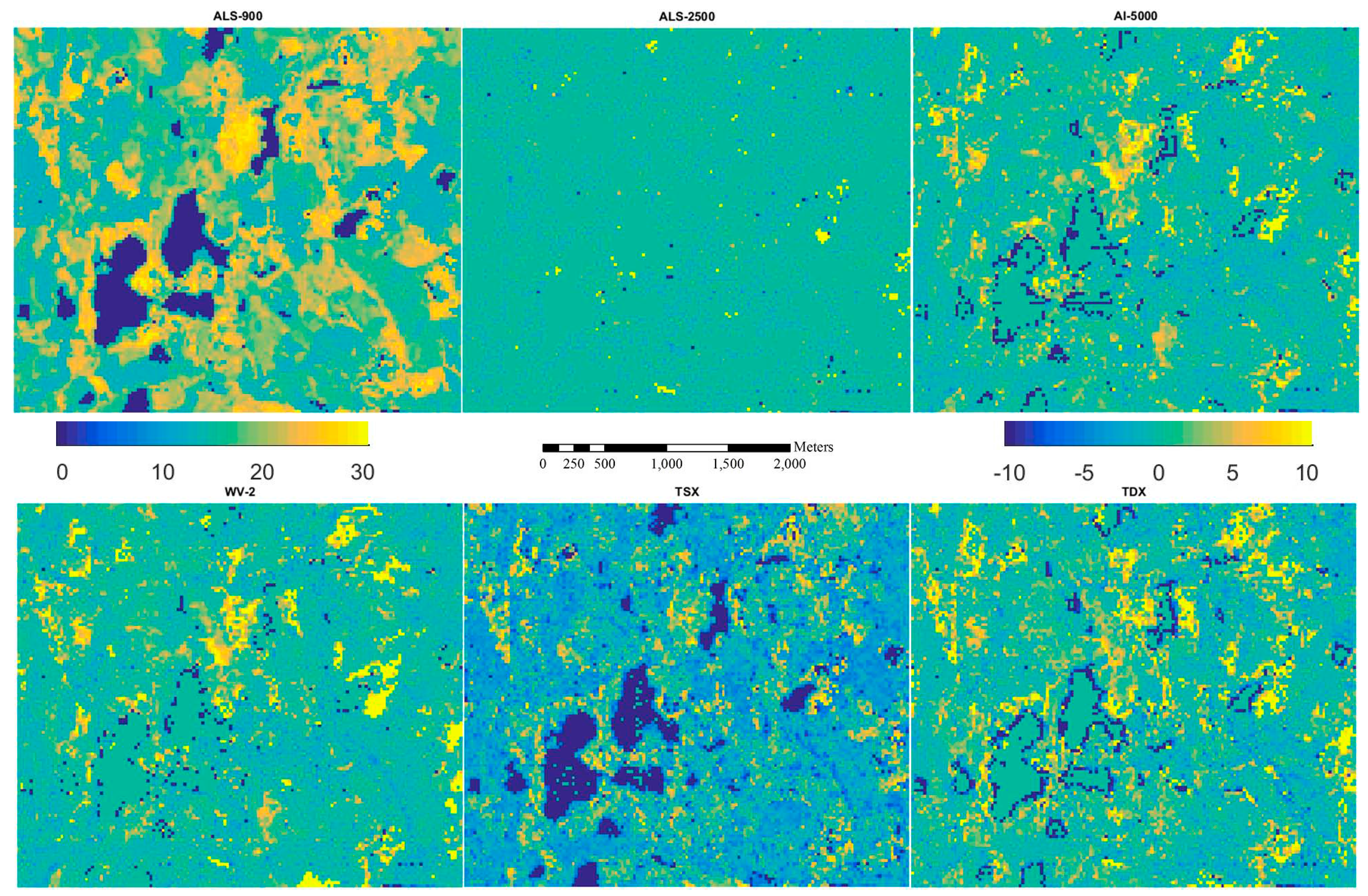
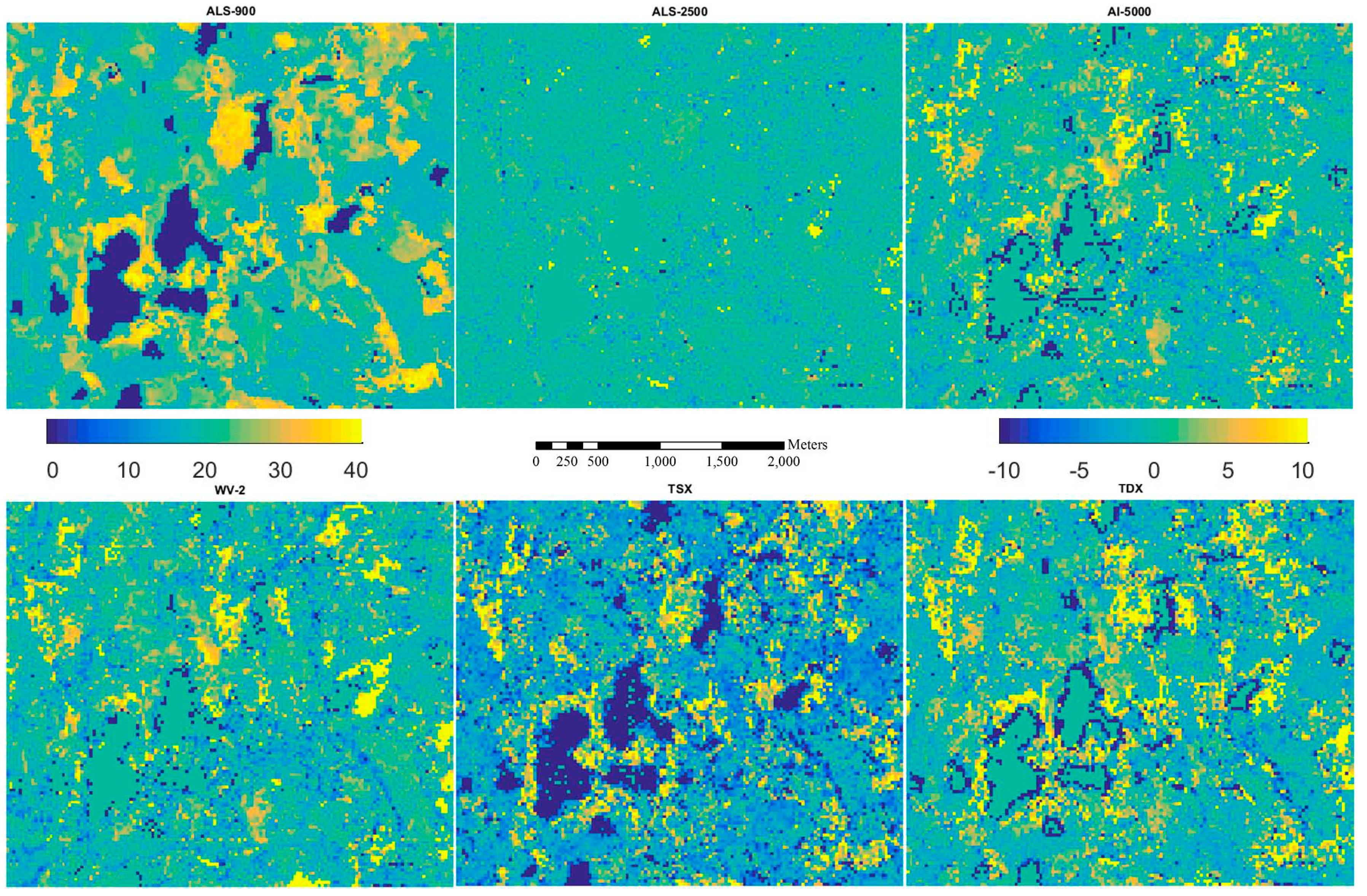
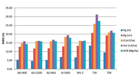
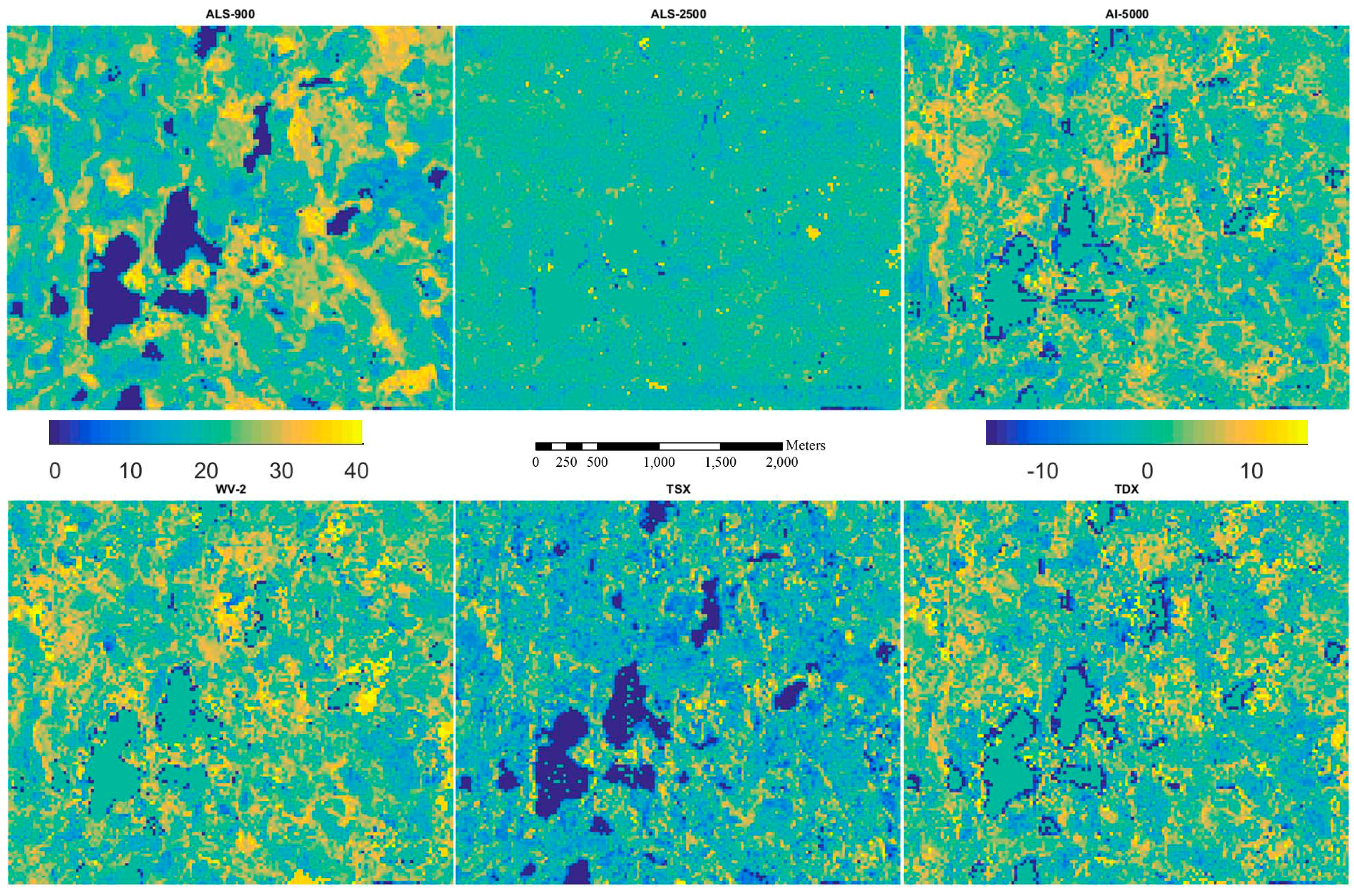
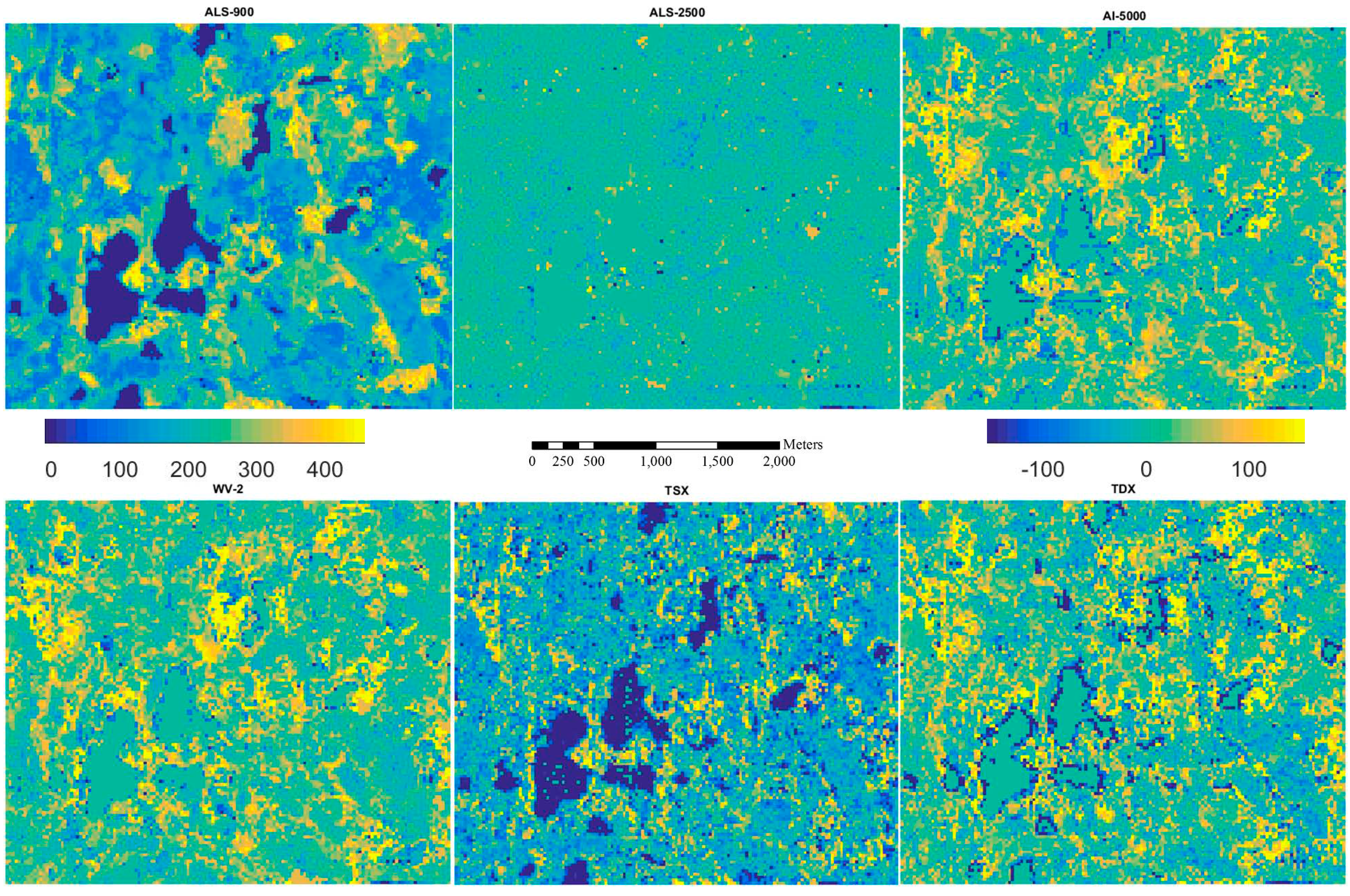
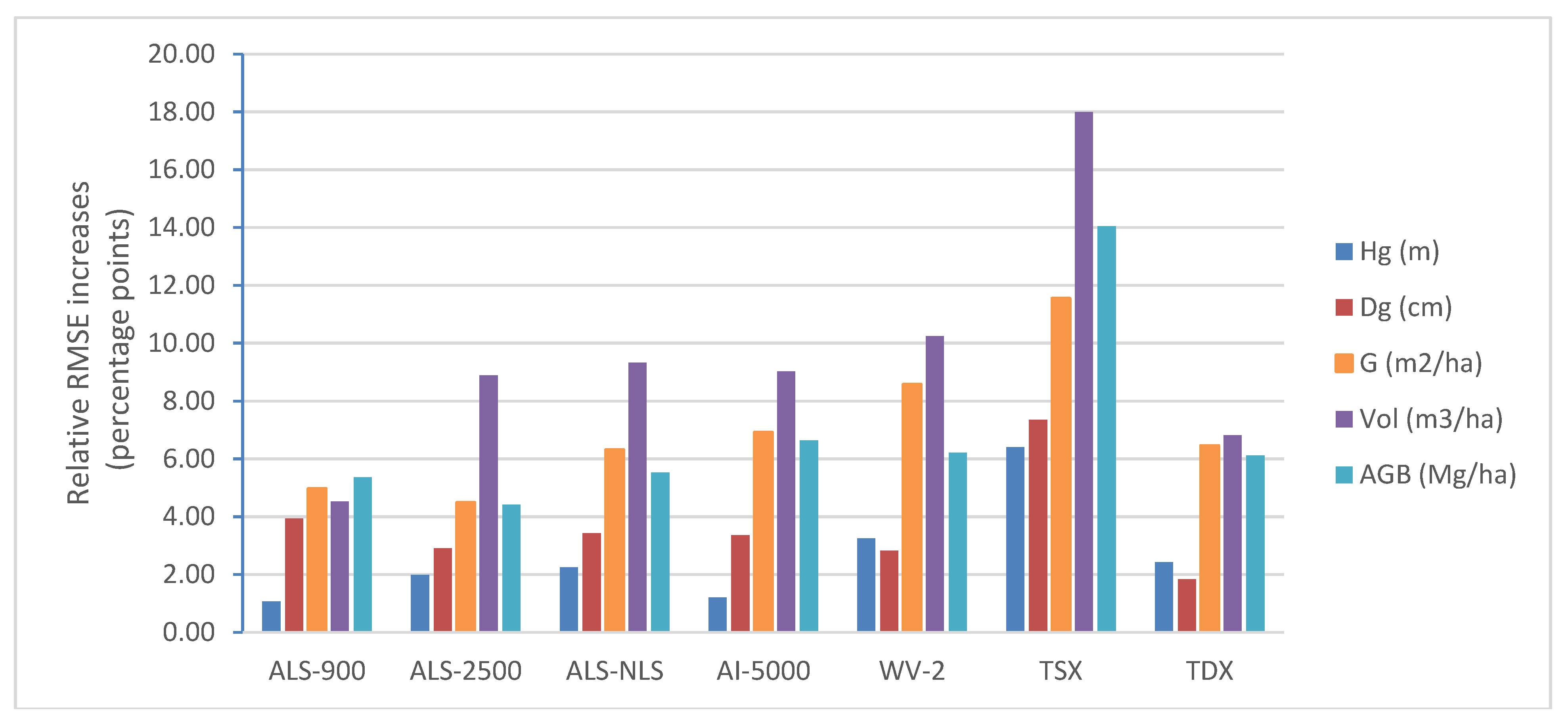
In this research, a comparison study was conducted to assess the explanatory power and information contents of several remote sensing data sources (laser scanning data, aerial images, WorldView-2 satellite images, SAR and InSAR) and methods providing 3D point clouds for the retrieval of plot level AGB, VOL, G, D_g and H_g. Results presented in this study showed that both space-borne and airborne 3D point clouds can be used for forest attribute mapping inventories. The relative RMSEs achieved were 4.6%–13.4% for H_g, 11.7%–20.6% for D_g, 14.8%–25.8% for G, 15.9%–31.2% for VOL and 14.3%–27.5% for AGB, respectively, depending on the data used. Overall results showed that ALS data produce the most accurate estimates for forest inventory attributes when compared with 3D point clouds generated from stereo airborne images using dense matching and space-borne radar images using radargrammetry and interferometry. However, the point density of ALS data is higher than image-based data. It is expected that estimation accuracy could be further improved with image-based point clouds when image resolution, radiometry and viewing geometry are improved. For example, WorldView-3 panchromatic imagery with a resolution of 0.3 m could produce a denser point cloud than WorldView-2 images. Features used in this study were originally developed for ALS point clouds. However, due to the nature of image-based clouds, i.e., the most of the points are created following the envelope of canopy, new features should be exploited in the future study although current set of the features performed well. When image-based data were compared, high altitude aerial images and WorldView-2 satellite images gave similar results, which were comparable to those obtained with ALS data. It seems that Interferometric SAR contains more information than radargrammetry SAR. Based on the analysis of plot size impact, we recommend predicting forest inventory attributes at a resolution greater than 500 m² when using image-based point clouds to achieve an acceptable accuracy level.

The major advantage of space-borne images, compared with airborne images or ALS, has been their availability and larger coverage. In the past, the saturation that occurs with higher biomass have restricted the use of optical and radar data in forest mapping. The results presented in this paper confirms usefulness of combination of airborne/space-borne images and 3D techniques as an option in developing methods for operational inventory and monitoring of large areas of forest attributes with improved accuracy and more frequent inventory cycles. Therefore, these alternative 3D techniques will be increasingly used supplementary to ALS in forest mapping and monitoring applications requiring high spatial accuracy at regional and country levels. It is anticipated that many of the future remote sensing processes for forestry will be based on 3D point cloud processing since canopy height information from forest is the main parameter remotely sensed data can provide for forest measurements. With its capability of penetration into the canopy, ALS is now the primary technique that is used for acquiring 3D information of vegetation, but other 3D techniques can be used to create forest attribute maps with accuracy close to ALS after high-quality DTM (created with ALS) exists from the areas of interest. When selecting the optimal data source, the costs of the data acquisition and of data preprocessing has to be taken into account in addition to the 3D point cloud processing costs, which is common to all of them. With the information of the expected accuracy, costs and availability of the data, foresters can select optimal/appropriate dataset for their purposes.

References

1. Hyyppä, J.; Inkinen, M. Detecting and estimating attributes for single trees using laser scanner. Photogramm. J. Finl. 1999, 16, 27–42. [Google Scholar]
2. Yu, X.; Hyyppä, J.; Vastaranta, M.; Holopainen, M.; Viitala, R. Predicting individual tree attributes from airborne laser point clouds based on random forests technique. ISPRS J. Photogramm. Remote Sens. 2011, 66, 28–37. [Google Scholar] [CrossRef]
3. Næsset, E. Estimating timber volume of forest stands using airborne laser scanner data. Remote Sens. Environ. 1997, 61, 246–253. [Google Scholar] [CrossRef]
4. Naesset, E. Predicting forest stand characteristics with airborne scanning laser using a practical two-stage procedure and field data. Remote Sens. Environ. 2002, 80, 88–99. [Google Scholar] [CrossRef]
5. Næsset, E. Determination of mean tree height of forest stands using airborne laser scanner data. ISPRS J. Photogramm. Remote Sens. 1997, 52, 49–56. [Google Scholar] [CrossRef]
6. Hyyppä, J.; Kelle, O.; Lehikoinen, M.; Inkinen, M. A segmentation-based method to retrieve stem volume estimates from 3-dimensional tree height models produced by laser scanner. IEEE Trans. Geosci. Remote Sens. 2001, 39, 969–975. [Google Scholar] [CrossRef]
7. Holmgren, J.; Persson, Å. Identifying species of individual trees using airborne laser scanning. Remote Sens. Environ. 2004, 90, 415–423. [Google Scholar] [CrossRef]
8. Brandtberg, T.; Warner, T.; Landenberger, R.; McGraw, J. Detection and analysis of individual leaf-off tree crowns in small footprint, high sampling density lidar data from the eastern deciduous forest in North America. Remote Sens. Environ. 2003, 85, 290–303. [Google Scholar] [CrossRef]
9. Hyyppä, J.; Yu, X.; Rönnholm, P.; Kaartinen, H.; Hyyppä, H. Factors affecting object-oriented forest growth estimates obtained using laser scanning. Photogramm. J. Finl. 2003, 18, 16–31. [Google Scholar]
10. Yu, X.; Hyyppä, J.; Kaartinen, H.; Maltamo, M. Automatic detection of harvested trees and determination of forest growth using airborne laser scanning. Remote Sens. Environ. 2004, 90, 451–462. [Google Scholar] [CrossRef]
11. Yu, X.; Hyyppä, J.; Kukko, A.; Maltamo, M.; Kaartinen, H. Change detection techniques for canopy height growth measurements using airborne laser scanner data. Photogramm. Eng. Remote Sens. 2006, 72, 1339–1348. [Google Scholar] [CrossRef]
12. Hyyppä, J.; Hyyppä, H.; Leckie, D.; Gougeon, F.; Yu, X.; Maltamo, M. Review of methods of small-footprint airborne laser scanning for extracting forest inventory data in boreal forests. Int. J. Remote Sens. 2008, 29, 1339–1366. [Google Scholar] [CrossRef]
13. Nurminen, K.; Karjalainen, M.; Yu, X.; Hyyppä, J.; Honkavaara, E. Performance of dense digital surface models based on image matching in the estimation of plot-level forest variables. ISPRS J. Photogram. Remote Sens. 2013, 83, 104–115. [Google Scholar] [CrossRef]
14. Honkavaara, E.; Markelin, L.; Rosnell, T.; Nurminen, K. Influence of solar elevation in radiometric and geometric performance of multispectral photogrammetry. ISPRS J. Photogramm. Remote Sens. 2012, 67, 13–26. [Google Scholar] [CrossRef]
15. Massonnet, D.; Feigl, K.L. Radar interferometry and its application to changes in the earth’s surface. Rev. Geophys. 1998, 36, 441–500. [Google Scholar] [CrossRef]
16. Rosen, P.A.; Hensley, S.; Joughin, I.R.; Li, F.K.; Madsen, S.N.; Rodriguez, E.; Goldstein, R.M. Synthetic aperture radar interferometry. Proc. IEEE 2000, 88, 333–382. [Google Scholar] [CrossRef]
17. Bohlin, J.; Wallerman, J.; Fransson, J.E.S. Forest variable estimation using photogrammetric matching of digital aerial images in combination with a high-resolution DEM. Scand. J. For. Res. 2012, 27, 692–699. [Google Scholar] [CrossRef]
18. Järnstedt, J.; Pekkarinen, A.; Tuominen, S.; Ginzler, C.; Holopainen, M.; Viitala, R. Forest variable estimation using a high-resolution digital surface model. ISPRS J. Photogram. Remote Sens. 2012, 74, 78–84. [Google Scholar] [CrossRef]
19. Vastaranta, M.; Wulder, M.A.; White, J.C.; Pekkarinen, A.; Tuominen, S.; Ginzler, C.; Kankare, V.; Holopainen, M.; Hyyppä, J.; Hyyppa, H. Airborne laser scanning and digital stereo imagery measures of forest structure: Comparative results and implications to forest mapping and inventory update. Can. J. Remote Sens. 2013, 39, 382–395. [Google Scholar] [CrossRef]
20. White, J.; Wulder, M.; Vastaranta, M.; Coops, N.; Pitt, D.; Woods, M. The utility of image-based point clouds for forest inventory: A comparison with airborne laser scanning. Forests 2013, 4, 518–536. [Google Scholar] [CrossRef]
21. Chen, Y.; Shi, P.; Deng, L.; Li, J. Generation of a top-of-canopy Digital Elevation Model (DEM) in tropical rain forest regions using radargrammetry. Int. J. Remote Sens. 2007, 28, 4345–4349. [Google Scholar] [CrossRef]
22. Perko, R.; Raggam, H.; Gutjahr, K.; Schardt, M. The capabilities of TerraSAR-X imagery for retrieval of forest parameters. ISPRS Int. Arch. Photogramm. Remote Sens. Spat. Inf. Sci. 2010, 38, 452–456. [Google Scholar]
23. Karjalainen, M.; Kankare, V.; Vastaranta, M.; Holopainen, M.; Hyyppä, J. Prediction of plot-level forest variables using TerraSAR-X stereo SAR data. Remote Sens. Environ. 2012, 17, 338–347. [Google Scholar] [CrossRef]
24. Persson, H.; Fransson, J.E. Forest variable estimation using radargrammetric processing of TerraSAR-X images in boreal forests. Remote Sens. 2014, 6, 2084–2107. [Google Scholar] [CrossRef]
25. Solberg, S.; Riegler, G.; Nonin, P. Estimating forest biomass from TerraSAR-X stripmap radargrammetry. IEEE Trans. Geosci. Remote Sens. 2015, 53, 154–161. [Google Scholar] [CrossRef]
26. Solberg, S.; Astrup, R.; Breidenbach, J.; Nilsen, B.; Weydahl, D. Monitoring spruce volume and biomass with InSAR data from TanDEM-X. Remote Sens. Environ. 2013, 139, 60–67. [Google Scholar] [CrossRef]
27. Karila, K.; Vastaranta, M.; Karjalainen, M.; Kaasalainen, S. Tandem-X interferometry in the prediction of forest inventory attributes in managed boreal forests. Remote Sens. Environ. 2015, 159, 259–268. [Google Scholar] [CrossRef]
28. Persson, H.; Wallerman, J.; Olsson, H.; Fransson, J.E.S. Estimating forest biomass and height using optical stereo satellite data and a DTM from laser scanning data. Can. J. Remote Sens. 2013, 39, 251–262. [Google Scholar] [CrossRef]
29. St-Onge, B.; Hu, Y.; Vega, C. Mapping the height and above-ground biomass of a mixed forest using lidar and stereo Ikonos images. Int. J. Remote Sens. 2008, 29, 1277–1294. [Google Scholar] [CrossRef]
30. Neigh, C.; Masek, J.; Bourget, P.; Cook, B.; Huang, C.; Rishmawi, K.; Zhao, F. Deciphering the precision of stereo IKONOS canopy height models for US forests with G-LiHT airborne lidar. Remote Sens. 2014, 6, 1762–1782. [Google Scholar] [CrossRef]
31. Montesano, P.M.; Sun, G.Q.; Dubayah, R.; Ranson, K.J. The uncertainty of plot-scale forest height estimates from complementary spaceborne observations in the taiga-tundra ecotone. Remote Sens. 2014, 6, 10070–10088. [Google Scholar] [CrossRef]
32. Rahlf, J.; Breidenbach, J.; Solberg, S.; Næsset, E.; Astrup, R. Comparison of four types of 3D data for timber volume estimation. Remote Sens. Environ. 2014, 155, 325–333. [Google Scholar] [CrossRef]
33. Laasasenaho, J. Taper Curve and Volume Functions for Pine, Spruce and Birch; Finnish Forest Research Institute: Helsinki, Finland, 1982. [Google Scholar]
34. Repola, J. Biomass equations for Scots pine and Norway spruce in Finland. Silva Fennica 2009, 43, 625–647. [Google Scholar] [CrossRef]
35. Axelsson, P. DEM generation from laser scanner data using adaptive TIN models. ISPRS Int. Arch. Photogramm. Remote Sens. Spat. Inf. Sci. 2000, 33, 110–117. [Google Scholar]
36. Hinz, A.; Dörstel, C.; Heier, H. DMC—The digital sensor technology of Z/I-Imaging. In Photogrammetric Week 2001, Proceedings of 48th Photogrammetric Week, Heidelberg, Germany, 24–28 September 2001; Fritsch, D., Spiller, R., Eds.; Wichmann Verlag: Heidelberg, Germany, 2001; pp. 93–103. [Google Scholar]
37. Jensen, J.L.R.; Humes, K.S.; Vierling, L.A.; Hudak, A.T. Discrete return lidar-based prediction of leaf area index in two conifer forests. Remote Sens. Environ. 2008, 112, 3947–3957. [Google Scholar] [CrossRef]
38. Kim, Y.; Yang, Z.; Cohen, W.B.; Pflugmacher, D.; Lauver, C.L.; Vankat, J.L. Distinguishing between live and dead standing tree biomass on the North Rim of Grand Canyon National Park, USA using small-footprint lidar data. Remote Sens. Environ. 2009, 113, 2499–2510. [Google Scholar] [CrossRef]
39. Yu, X.; Hyyppä, J.; Holopainen, M.; Vastaranta, M. Comparison of area-based and individual tree-based methods for predicting plot-level forest attributes. Remote Sens. 2010, 2, 1481–1495. [Google Scholar] [CrossRef]
40. Vastaranta, M.; Kankare, V.; Holopainen, M.; Yu, X.; Hyyppä, J.; Hyyppä, H. Combination of individual tree detection and area-based approach in imputation of forest variables using airborne laser data. ISPRS Photogramm. Remote Sens. 2012, 67, 73–79. [Google Scholar] [CrossRef]
41. Breiman, L. Random forests. Mach. Learn. 2001, 45, 5–32. [Google Scholar] [CrossRef]
42. Baltsavias, E.; Gruen, A.; Eisenbeiss, H.; Zhang, L.; Waser, L.T. High-quality image matching and automated generation of 3D tree models. Int. J. Remote Sens. 2008, 29, 1243–1259. [Google Scholar] [CrossRef]
43. Fransson, J.E.S.; Israelsson, H. Estimation of stem volume in boreal forests using ERS-1 C- and JERS-1 L-band SAR data. Int. J. Remote Sens. 1999, 20, 123–137. [Google Scholar] [CrossRef]
44. Holopainen, M.; Haapanen, E.; Karjalainen, M.; Vastaranta, M.; Hyyppä, J.; Yu, X.; Tuominen, S.; Hyyppä, H. Comparing accuracy of airborne laser scanning and TerraSAR-x radar images in the estimation of plot-level forest variables. Remote Sens. 2010, 2, 432–445. [Google Scholar] [CrossRef] [Green Version]