Automated Recognition of Railroad Infrastructure in Rural Areas from LIDAR Data

Abstract

This study is aimed at developing automated methods to recognize railroad infrastructure from 3D LIDAR data. Railroad infrastructure includes rail tracks, contact cables, catenary cables, return current cables, masts, and cantilevers. The LIDAR dataset used in this study is acquired by placing an Optech Lynx mobile mapping system on a railcar, operating at 125 km/h. The acquired dataset covers 550 meters of Austrian rural railroad corridor comprising 31 railroad key elements and containing only spatial information. The proposed methodology recognizes key components of the railroad corridor based on their physical shape, geometrical properties, and the topological relationships among them. The developed algorithms managed to recognize all key components of the railroad infrastructure, including two rail tracks, thirteen masts, thirteen cantilevers, one contact cable, one catenary cable, and one return current cable. The results are presented and discussed both at object level and at point cloud level. The results indicate that 100% accuracy and 100% precision at the object level and an average of 96.4% accuracy and an average of 97.1% precision at point cloud level are achieved.

1. Introduction

Railroad transportation constitutes a large portion of travels around the globe. In the USA, for instance, 476 million passengers use railroad transportation annually, and Japan being the first in the world with 22.67 billion passengers annually [1]. In addition to passenger transportations, freight rail also forms a large portion of total freight in the world. In the USA freight rail composes 42% of its total freight, while Russian freight rail makes up 65% of its total freight (standing as the first in the world) [1]. The safety of railroad corridors is a crucial issue. In 2014, train accidents were 15% of all reported incidents in the USA. This comprised 1246 derailments (i.e., incidents in which a train ran off rail tracks), causing 804 fatalities (deceased individuals) and 8504 non-fatal injuries (injured individuals). Moreover, in the same year, forty railroad incidents resulted in the release of hazardous materials [2]. This portrays a thorough picture of the consequences of lack of security in the railroad corridors and implies an urgent need to take appropriate measures to improve the safety of railroad corridors. Rails defects (29%) and equipment failure (13%) are the second and third leading causes of rail accidents, after human factors (38%) as the primary cause [3]. Defects of rails and equipment can be due to various reasons, such as wear and tear, problematic ecosystem, etc. Problematic ecosystem occurs when the required clearance around a railroad corridor is violated by the surrounding vegetation; giant tree roots that destabilize the track bed’s sub-grade materials or unchecked vegetation growth that interfere with trains in motion are two instances of a problematic ecosystem.

Regular monitoring of the railroad infrastructure can be a comprehensive solution to address the safety issues in this environment. By regular inspection, the current state of the infrastructure will be monitored, and problematic ecosystems can also be identified. This is currently carried out in many countries in a traditional way by staff that traverse along railroads and visually inspect the current state of the railroads. For instance, the USA federal railroad administration (FRA) requires the rail tracks to be inspected as often as twice per week [4]. Traditional monitoring of railroad corridors is, however, quite slow, costly, and sometimes erroneous, due to human mistakes.

This study aims to develop automated methods to recognize key components of railroad infrastructure from 3D LIDAR data. The results of this work can be utilized to automate the monitoring of the railroads, which improves the safety and significantly lowers the maintenance costs. LIDAR data is acquired by a mobile mapping system (mounted on a train), which scans the railroads while the train is moving. Furthermore, the results of this research can be utilized for the future design enhancements such as rail siding operations (laying additional rail tracks next to the existing tracks). Rail siding is carried out to improve the flow of the rail traffic and it requires a precise and accurate survey of the existing state of railroad corridors.

2. Literature Review

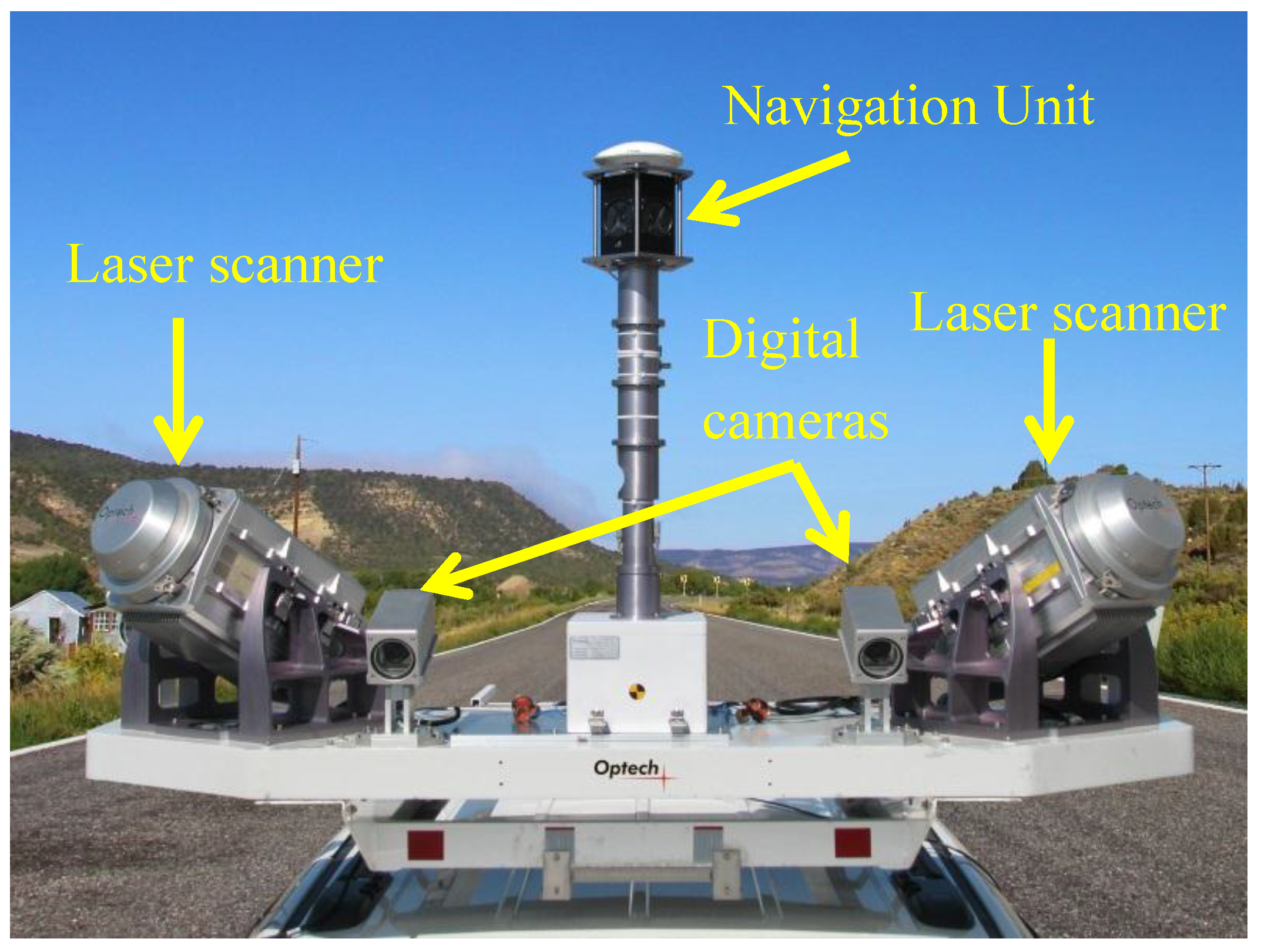
Mobile mapping systems (MLS) are composed of an imaging unit (incorporating laser scanners and/or digital cameras) and a navigation unit (including GNSS and INS systems) for spatial referencing. Accordingly, mobile mapping is defined as a task of capturing and providing 3D geometric information using an imaging sensor attached to a moving platform. The platform is typically mounted on a motor vehicle such as a train, a car, etc. In mobile mapping systems, while the platform is moving along a trajectory, the laser scanner is continuously scanning a 2D profile [5]. There are various mobile mapping systems with different sensors and configuration [6,7]. Generally, laser beams are categorized in four major classes based on their safety risks. The higher the class, the more powerful the laser beam, which potentially poses serious danger to the eyes. Mobile mapping laser scanners fall in the third category in which laser beams can be momentarily hazardous once directly viewed or stared at with an unaided eye. However, the contact of the laser beam with other parts of human body is quite safe [8].

Laser scanners collect data by laser range finding i.e., emitting a laser beam and measuring the time of flight or the phase change of the reflected beam. When a laser scanner is operating, its head rotates perpendicular to its platform’s normal axis and its oscillating mirror deflects the laser beam to sweep the surrounding environment. Then 3D co-ordinates of points are computed using the observed range and the angle of the oscillating mirror. 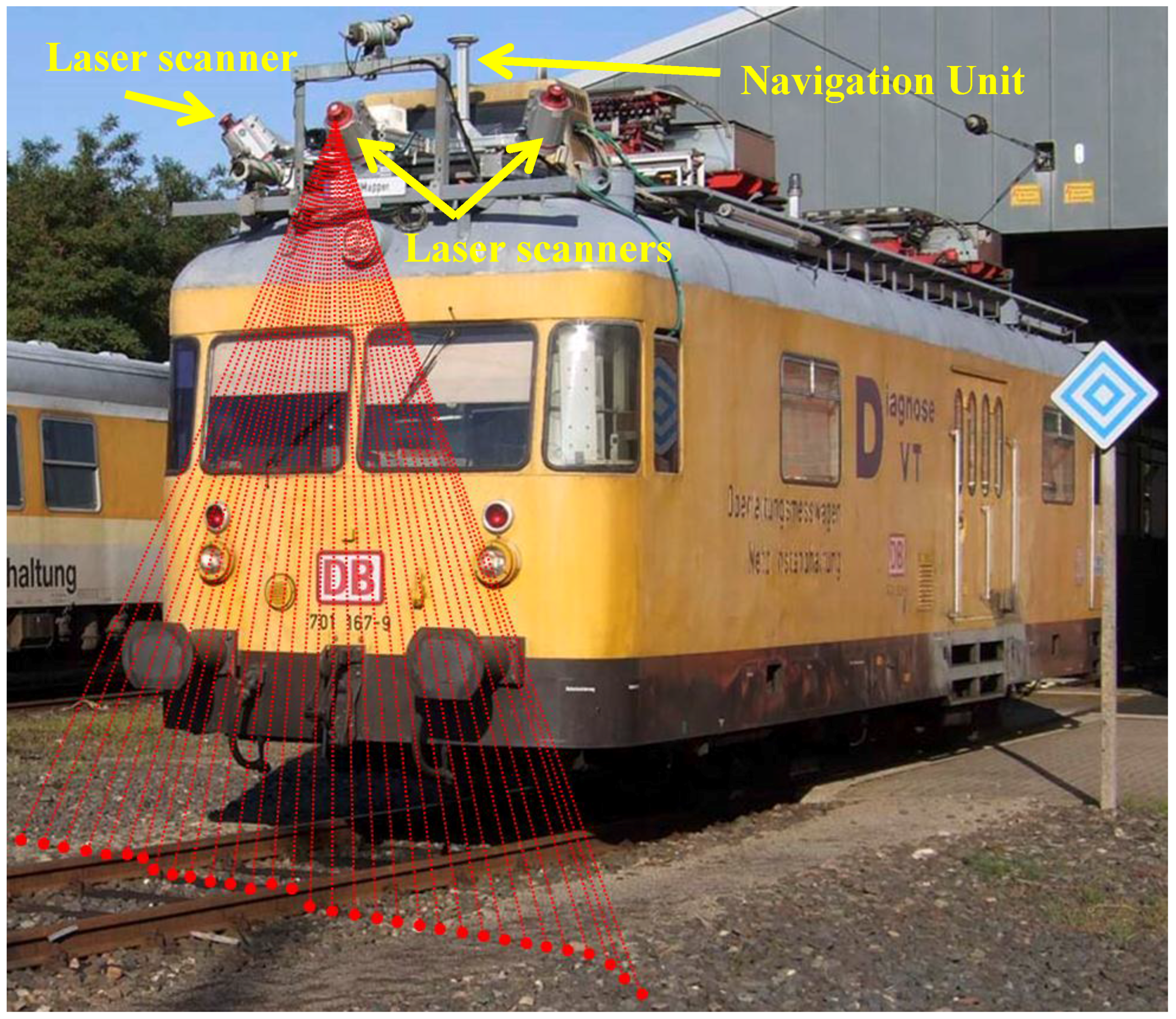Figure 1 indicates a sample mobile mapping system mounted on a train with three laser scanners and a navigation unit. While this figure demonstrates one example of scanning of the track bed and rail tracks, mobile mappers’ laser sensors usually offer a 360° field of view that scans all objects in railroad corridors, including the track bed, rail tracks, over-head power cables, masts, and surrounding vegetation, etc.

Figure 1. A sample mobile mapping system mounted on a train with three laser scanners and one navigation unit. A sample scanning pattern of one of the laser scanners is shown in red [9].

Figure 1. A sample mobile mapping system mounted on a train with three laser scanners and one navigation unit. A sample scanning pattern of one of the laser scanners is shown in red [9].

The resulting dataset of a mobile mapping system is a geo-referenced point cloud i.e., a set of points with 3D co-ordinates in a global spatial reference system (GSRF) or a national spatial reference system (NSRF), with or without additional data, such as intensity data and RGB data of the integrated digital cameras. Next, the resulting point cloud needs to be processed for which many methods exist (see Otepka et al. [10]). To this end, segmentation needs to be carried out to cluster points so that objects of interest can be recognized. A spatial-domain method (region-growing) is employed for the segmentation part. Spatial-domain methods are computationally less intense and, thus, more efficient, compared to parametric-domain methods, such as the Hough Transform [11].

This paragraph reviews the most relevant works on the recognition of railroad infrastructure, as well as studies on object recognition in environments with objects similar to railroad infrastructure. Morgan [12] discusses only the potential of using LIDAR data in monitoring railroads and the surrounding environment. Morgan, however, does not propose an automated methodology to do so and the focus is limited to visualizing the acquired LIDAR data and the information that can be inferred by visual inspection. Lesler et al. [13] discuss employing a MLS system to survey railroad corridors by scanning 32 miles of American freight rail corridor. However, the data processing is carried out manually by using commercial software. Soni et al. [14] manually model rail tracks. They scan rail tracks close to a train station with a terrestrial laser scanner and fit 3D CAD models to manually-extracted rail tracks using commercial software. Beger et al. [15], Neubert et al. [16], and Miao et al. [17] extract railroad centerlines using LIDAR datasets and high-resolution aerial imagery employing image processing techniques. Sawadisavi et al. [4] use imagery and machine vision technology to detect the irregularities and defects in railroad infrastructures. Zhu and Hyyppa [18] recognize objects surrounding railroad corridors i.e., terrain, roads, buildings, trees, etc. Rail tracks, however, are not the objects of interest and, thus, are not recognized. They integrate airborne LIDAR data and MLS data and then convert the integrated data to images and employ image processing techniques. Jwa et al. [19] propose an algorithm to reconstruct power cables based on a voxel-based piece-wise line detector. They enhanced their algorithm in the following year to avoid under- and over-segmentations by applying a multi-level span analysis [20]. Power cables in [19] and [20] are recognized by using polynomial functions to fit models to catenaries. The recognized cables in these two studies are similar to overhead power cables in railroad environments in physical shape. Lehtomaki et al. [21] propose a multi-step methodology to extract poles in a road environment. A scan line segmentation method is carried out based on proximity of points and then poles are detected based on the size, shape, and orientation of the resulting segments. Vertical poles are one of the railroad corridors’ key components. Yang and Fang [22] recognize rail tracks by using geometry and intensity data. They focus only on the extraction of rail tracks and other objects are not recognized. They also use structured point clouds (scan lines) in the recognition of some objects, such as the track bed. Elberink and Khoshelham [23] propose a model-driven approach to extract and model rail track centerlines. First, they coarsely extract the rail tracks by using local properties of rails such as height and parallelism, and then fine extraction is carried out in the modelling step. Moreover, other rail corridors’ elements are not extracted since their primary focus is on the rail track recognition. Elberink and Khoshelham [23] improved their earlier work [24] which deals with a simpler railroad configuration.

The majority of the past studies focus only on the extraction of rail track centerlines and other railroad infrastructure are not recognized. They also usually take advantage of other sources of information, such as imagery, intensity data, RGB data, and airborne LIDAR data. This study is, however, aimed at developing a comprehensive data-driven approach for fully-automated recognition of all components of railroad infrastructure. Moreover, this work is intended to use only unstructured MLS point clouds containing only geometry data i.e., unstructured points with 3D co-ordinates with no imagery, intensity, scan lines, or RGB data. Data-driven approaches are computationally less intense than model-driven approaches; this is because, in data-driven approaches local properties are usually inspected and, thus, a smaller number of points are processed. Model-driven approaches involve modelling and line and/or curve fitting to a large number of points, which is computationally intense. However, model-driven approaches have advantages as well. For instance, they produce better results once the dataset point sampling of is quite poor. Furthermore, model-driven approaches are very useful to recognize parameterized-shape objects that are composed of geometric primitives such as planes and cylinders. Since the physical shape of railroad elements is more complicated than those of geometric primitives, and the data used in this study is well-sampled, a data-driven approach is used in this work.

3. Methodology

Recognition of each type of object is composed of three primary steps: inspecting local neighbourhoods; classification; and segmentation. Studying local neighbourhoods requires seeking for the neighbourhood of each point, which can be computationally intense. To increase the efficiency of a neighbourhood search, a K dimensional (KD) tree data structure [25] is constructed and the nearest neighbour search for each query point is performed employing a fast library for approximate nearest neighbours (FLANN) algorithm [26], implemented in the C++ programming language. A neighbourhood search is carried out as a radius search i.e., seeking for points in a certain 3D Euclidean distance of a query point (see Otepka et al. [10]). That is, a point $P_i$ belongs to the neighbourhood of point P₀ ($N_{P_{\circ }}$) if their 3D Euclidean distance is equal to or less than a certain radius (r), as in Equation (1).

$$P_i\in N_{P_{\circ }}if\sqrt{{(x_{P_i}-x_{P\circ })}^2+{(y_{P_i}-y_{P\circ })}^2+{(z_{P_i}-z_{P_{\circ }})}^2}\le r$$

(1)

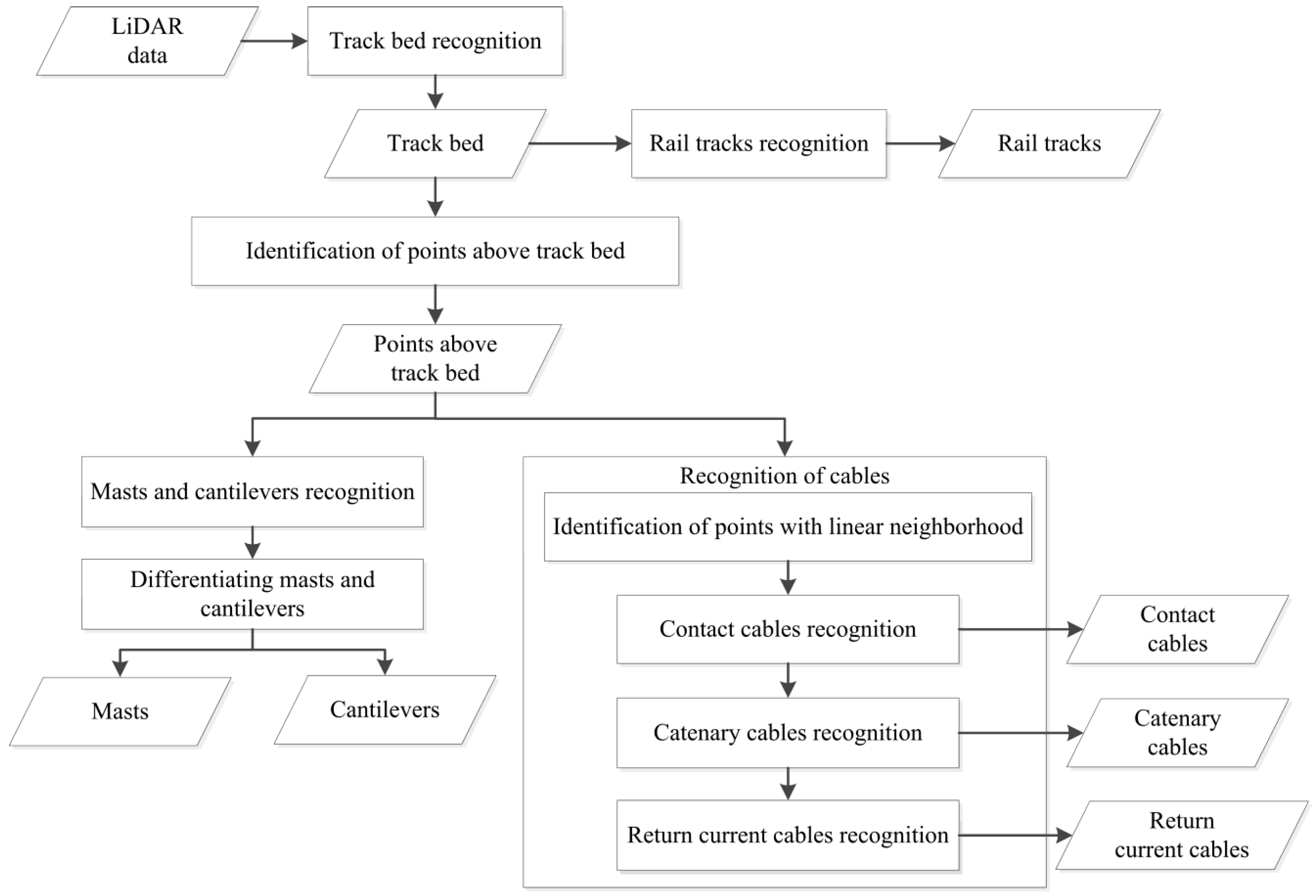
Classification is carried out by developing and applying constraints based on three information cues: local neighbourhood structure; shape of objects; and topological relationships among objects. Afterwards, segmentation is carried out by clustering the classified points i.e., points identified as belonging to an object type. Figure 2 presents the flowchart of the proposed methodology.

Figure 2. Flowchart of the proposed methodology.

Figure 2. Flowchart of the proposed methodology.

The methodology is described in five sections. Section 3.1 introduces the railroad infrastructure components and the following sections detail the methodology to recognize each component type.

3.1. Components of Railroad Infrastructure

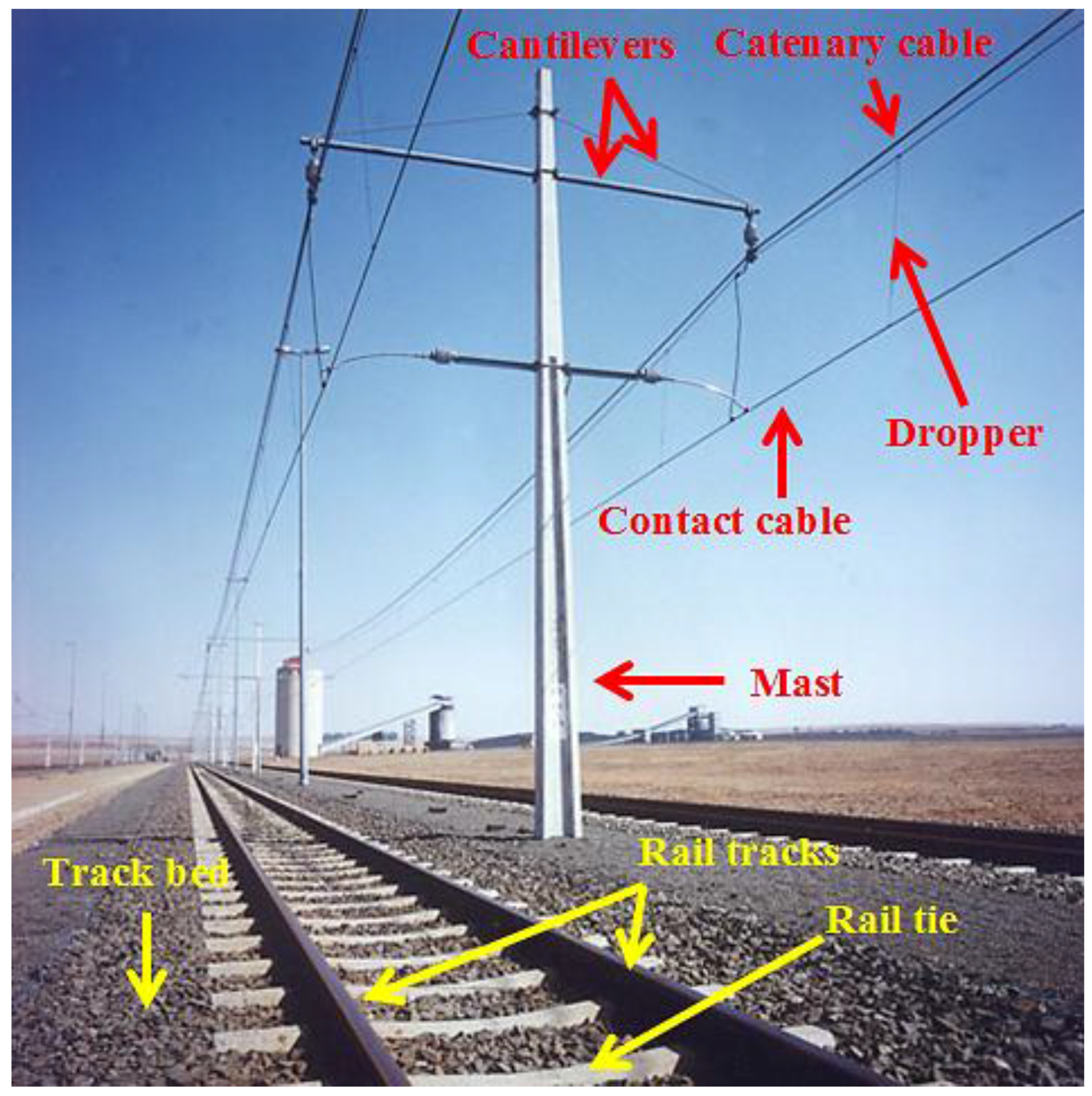
Key components of railroad corridors comprise rail tracks, overhead power cables (contact cables, catenary cables, and return current cables), masts, and cantilevers, shown in Figure 3. Recognition of other components such as ballast, railroad ties, and droppers are not in the scope of this work.

Figure 3. Components of Railroad Infrastructure [27].

Figure 3. Components of Railroad Infrastructure [27].

• Track Bed

The track bed is the surface underlying rail tracks and consists of a sub-grade level topped with ballast, which holds rail tracks in line and on the surface. Ballast consists of sized hard particles easily handled in tamping, which distribute the load, drain well, and resist plant growth [28]. The track bed is not a key element of railroad corridors. It, however, has a key role in the recognition of other components.

The track bed represents the areal extent of the railroad corridors since the rail tracks lie within its areal extent, overhead power cables lie above it and masts are located in its very close proximity. Therefore, the track bed is the first object to be recognized.

• Rail Tracks

Rail tracks are rolled-shaped steel designed to be laid end-to-end in two parallel lines on which trains are able to move. The standard European gauge (spatial offset between a pair of rail tracks) is 1.435 m [29] and the standard European track height is between 142 mm and 172 mm [30].

• Overhead Power Cables

Contact cables, catenary cables, droppers, and return current cables are four elements of the overhead power cables. Contact cables, the lowest in height among all overhead power cables, are energized by electricity and transmit the power to trains. Catenary cables are a system of curve-shaped cables suspended between poles (called masts). They lie immediately above contact cables and hold them in place by droppers. Return current cables lie highest among all power cables and are connected to the topmost part of the masts. Similar to catenary cables, return current cables are curvilinear cables that are suspended from topmost part of the masts.

• Mast and Cantilevers

Masts are poles located in regular spatial intervals in a close proximity of rail tracks. They provide support for the suspended overhead power cables to hold them in place. Cantilevers are metal support tubes that are employed to connect masts to catenaries.

3.2. Recognition of the Track Bed

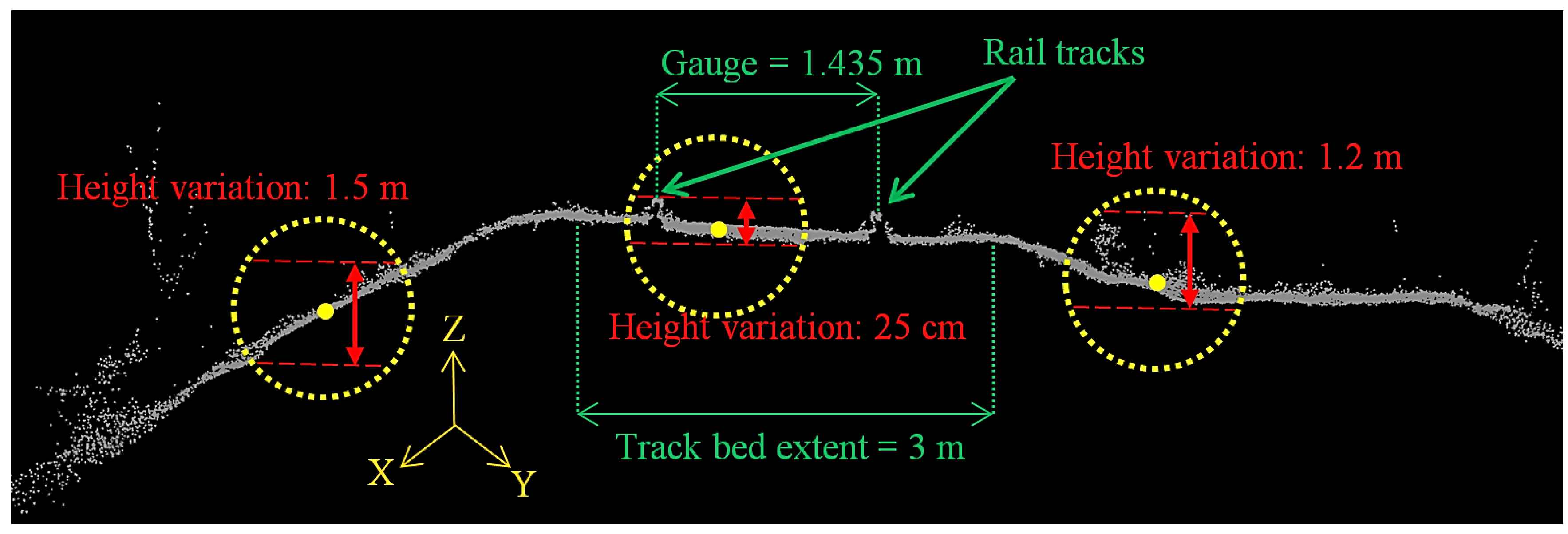
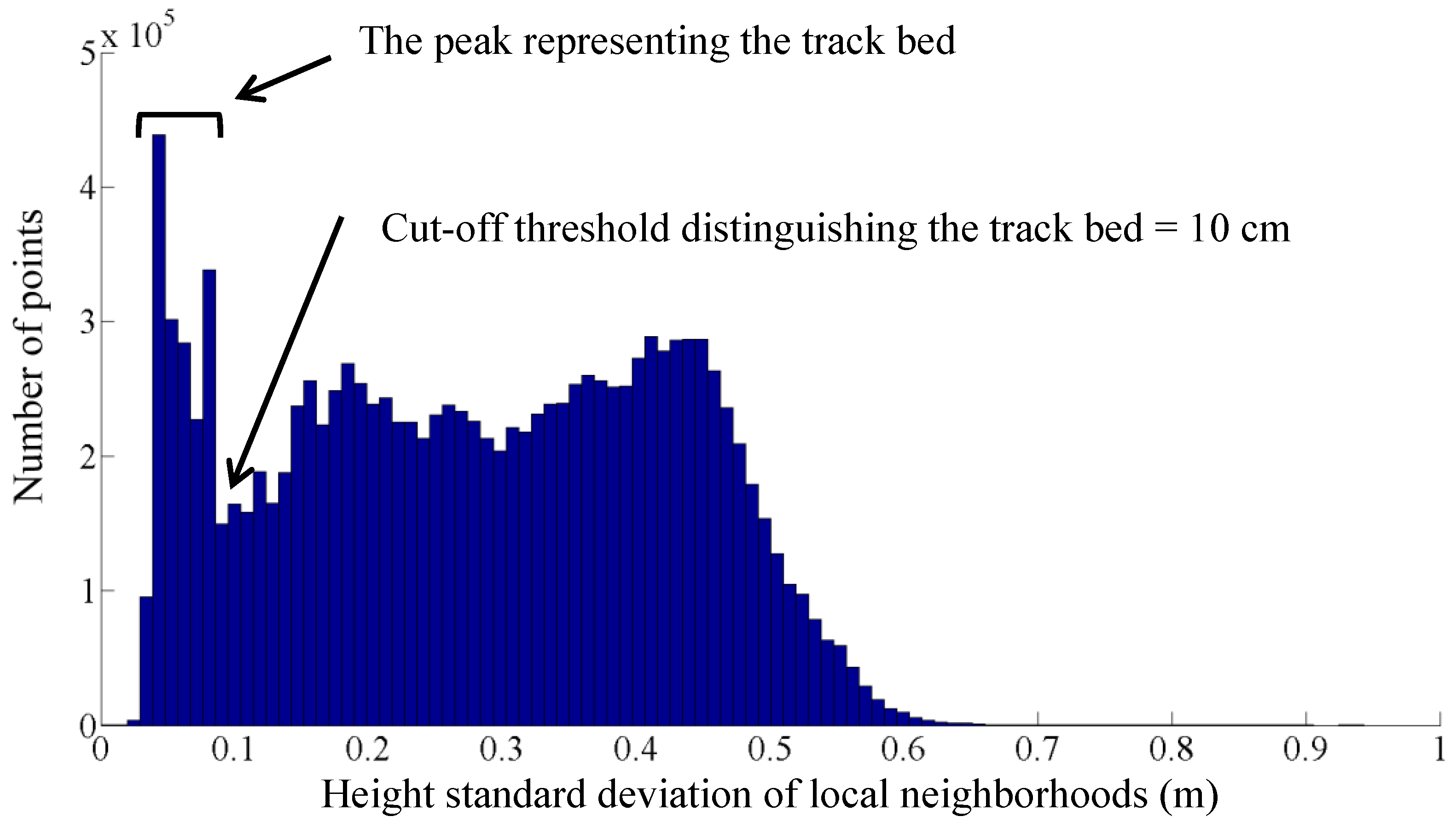
Due to safety reasons, the track bed is designed and constructed to be a surface with the smallest height variation possible to provide a safe and stable platform for trains in motion. Figure 4 shows a side view (vertical cross section) of the track bed that clearly indicates points on track bed have much smaller height variation, compared to other parts of the dataset. The track bed is recognized by identifying points with uniform-height neighbourhood. The developed algorithm recognizes points belonging to the track bed by investigating the histogram of the height standard deviation of each point’s neighbourhood. Such a histogram is indicated in Figure 5. Since points on the track bed have the smallest height variation in the data, they form a peak in the leftmost side of the histogram. The algorithm detects this peak and then looks for a sudden drop in the bin’s value to the right of the peak. The sudden drop in the histogram gradient provides a threshold that differentiates the peak (representing the track bed points) from the remaining histogram (representing non-track bed points). As a result, points whose neighbourhood have a height standard deviation equal to or less than the determined threshold are recognized as track bed candidate points. The neighbourhood size needs to be large enough to provide true properties of local neighbourhoods. Furthermore, if the neighbourhood size is smaller than the track gauge, a maximum of one rail track falls in each neighbourhood that makes the recognition more successful. Herein, the neighbourhood size is considered one meter so that it covers a maximum of one rail track, considering European standard track gauge (1.435 m). In addition, considering the dataset point sampling (detailed in Section 4), one meter neighbourhood size reflects reliable information regarding the local height variation. The bin size of the histogram is one centimeter. It is required to note that bin size only affects the precision of the determined threshold and points on the track bed form a peak on the leftmost part of the histogram regardless of the bin size.

Candidate points need to be further processed to recognize the true track bed points since points on the track bed are not the only points with small height variation. Points on cables and some surrounding vegetation also have a uniform-height neighbourhood. Thus, all candidate points in 20-cm 3D Euclidean distance of one another are clustered. Due to the size of the track bed and its continuity, points on the track bed form the largest segment. Therefore, the largest segment is deemed to belong to the track bed. It should be noted that points that are identified as belonging to the track bed in this section include points on rail tracks as well. Therefore, in Section 3.3 only points that are identified as belonging to the track bed (in this section) are further processed to separate points on rail tracks from points on the track bed.

Figure 4. Height variation in various parts of the railroad corridor. Yellow points and yellow dashed circles represent sample query points and their corresponding 3D spherical neighbourhood and double arrows depict the height variation within each local neighbourhood.

Figure 4. Height variation in various parts of the railroad corridor. Yellow points and yellow dashed circles represent sample query points and their corresponding 3D spherical neighbourhood and double arrows depict the height variation within each local neighbourhood.

Figure 5. Histogram of height standard deviation of local neighbourhoods.

Figure 5. Histogram of height standard deviation of local neighbourhoods.

The clustering distance threshold (20 cm) is selected based on point sampling of the dataset (discussed in Section 4) and the dimensions and spatial offset among various objects in the railroad corridor. It provides reliable information regarding the neighbourhood under inspection without including points from other objects. The 20-cm distance threshold is used for the majority of neighbourhood sizes and distance thresholds of the clustering algorithms in different parts of the proposed methodology in this work. Once a different threshold is used, its exact value is mentioned and its rationale is accordingly justified.

3.3. Recognition of Rail Tracks

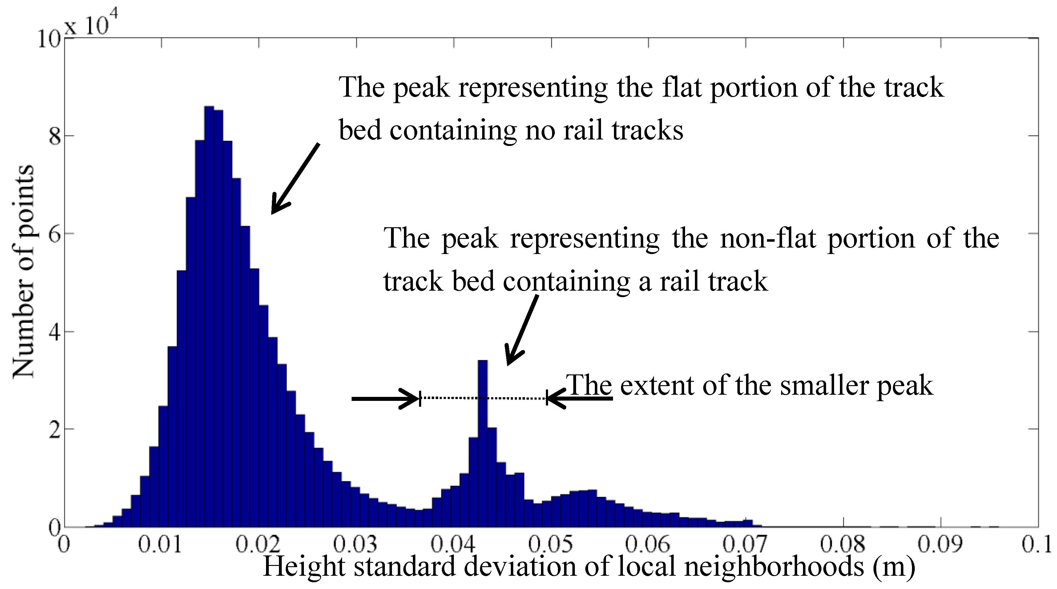
Rail tracks are recognized by considering their three primary properties: causing height variation on the track bed; continuity; and smooth curvature gradient. Continuity and smooth curvature gradient of rail tracks are enforced due to safety restrictions. First, the height variation of points on the track bed is inspected by computing the histogram of the height standard deviation of each point’s neighbourhood. Two main peaks are expected in the histogram; one peak with very small height variation (representing points on flat portion of the track bed with no rails) and another peak with slightly larger height variation (representing points on non-flat portion of the track bed with rail tracks). The former constitutes a larger peak since the number of points on flat portion of the track bed is much larger than the number of points on non-flat portion (rail tracks). Figure 6 indicates such a histogram in which two primary peaks can be conveniently visualized. The developed algorithm automatically recognizes the extent of the smaller peak by seeking for two abrupt drops in the histogram gradient (bin values) to its both left and right sides. Points whose height standard deviation is in the extent of the smaller peak are considered as candidate rail track points. The 20-cm neighbourhood size utilized in previous section is also applicable in this section. That is since the neighbourhood size needs to be larger than rail vertical dimension (height) so that the height variation introduced by rail tracks is reflected in the histogram. As mentioned in the second part of Section 3.1, the height of standard European rails are between 142 mm and 172 mm that is smaller than the considered 20-cm neighbourhood size.

Figure 6. Histogram of height standard deviation of points on the track bed.

Figure 6. Histogram of height standard deviation of points on the track bed.

Afterwards, candidate rail points that are within 20-cm 3D Euclidean distance from one another are clustered. Some false positives are expected due to various reasons such as external objects and grown vegetation on the track bed. Moreover, some parts of rails might be un-recognized, which result in over-segmentation. Therefore, a region growing algorithm is developed to integrate the recognized rail segments and also to exclude false positives. The algorithm starts by considering a random rail segment (let us call it “growing segment” i.e., GS) and finding rail segments within its one-meter neighbourhood (let us call them “candidate segments” i.e., CS). The vector connecting the closest points on a GS and each of its CSs (connecting points) are computed (${\overrightarrow{V}}_i$) and then the direction vector of the GS on its connecting point is calculated (${\overrightarrow{W}}_i$). If the angle between ${\overrightarrow{W}}_i$ and ${\overrightarrow{V}}_i$ is less than 20°, the CS under inspection is integrated with the GS. 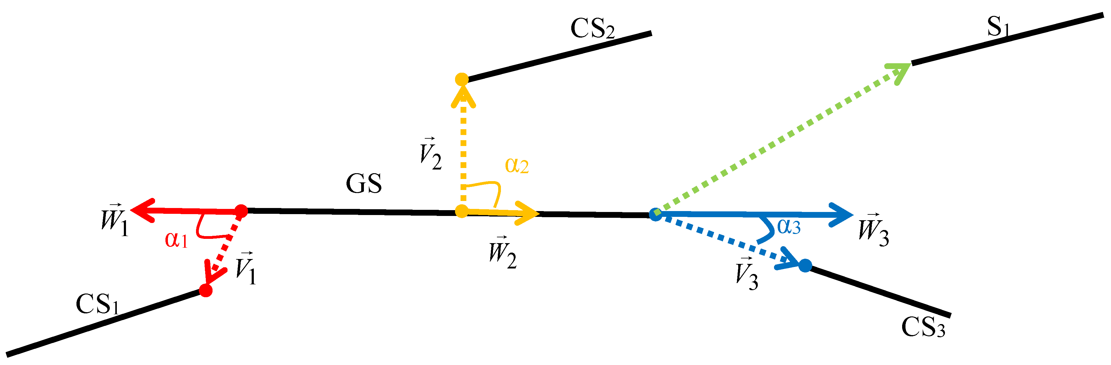Figure 7 indicates a GS with four segments around it, in which the two connecting points of the GS and each of the CSs are shown by different colors. Additionally, the solid arrows represent the direction of the GS on its connecting point (${\overrightarrow{W}}_i$), the dashed arrows represent the vector connecting the closest points of the GS and a CS (${\overrightarrow{V}}_i$), and ${\alpha }_i$ is the angle between these two vectors. ${\alpha }_1$ and ${\alpha }_2$ are too large, implying that the CS₁ and CS₂ are not along the GS and, thus, should not be merged. ${\alpha }_3$; however, is in the acceptable range implying that CS₃ is in line with the GS and should be merged. S₁ is not a candidate segment and is ignored since it is not within one-meter neighbourhood of the GS.

Thresholds utilized in the region growing algorithm are derived from rail tracks properties, such as track gauge and track curvature gradient. Distance threshold (one meter) is selected by considering the track gauge (1.435 m) to avoid integrating points belonging to adjacent rail tracks and the angle threshold (20°) is chosen by considering the maximum curvature of an one-meter long rail track.

Figure 7. The growing rail segment (GS) would be merged only with candidate segment three (CS₃) since other candidate segments are either too far from GS or they are not in line with GS.

Figure 7. The growing rail segment (GS) would be merged only with candidate segment three (CS₃) since other candidate segments are either too far from GS or they are not in line with GS.

3.4. Recognition of Overhead Power Cables

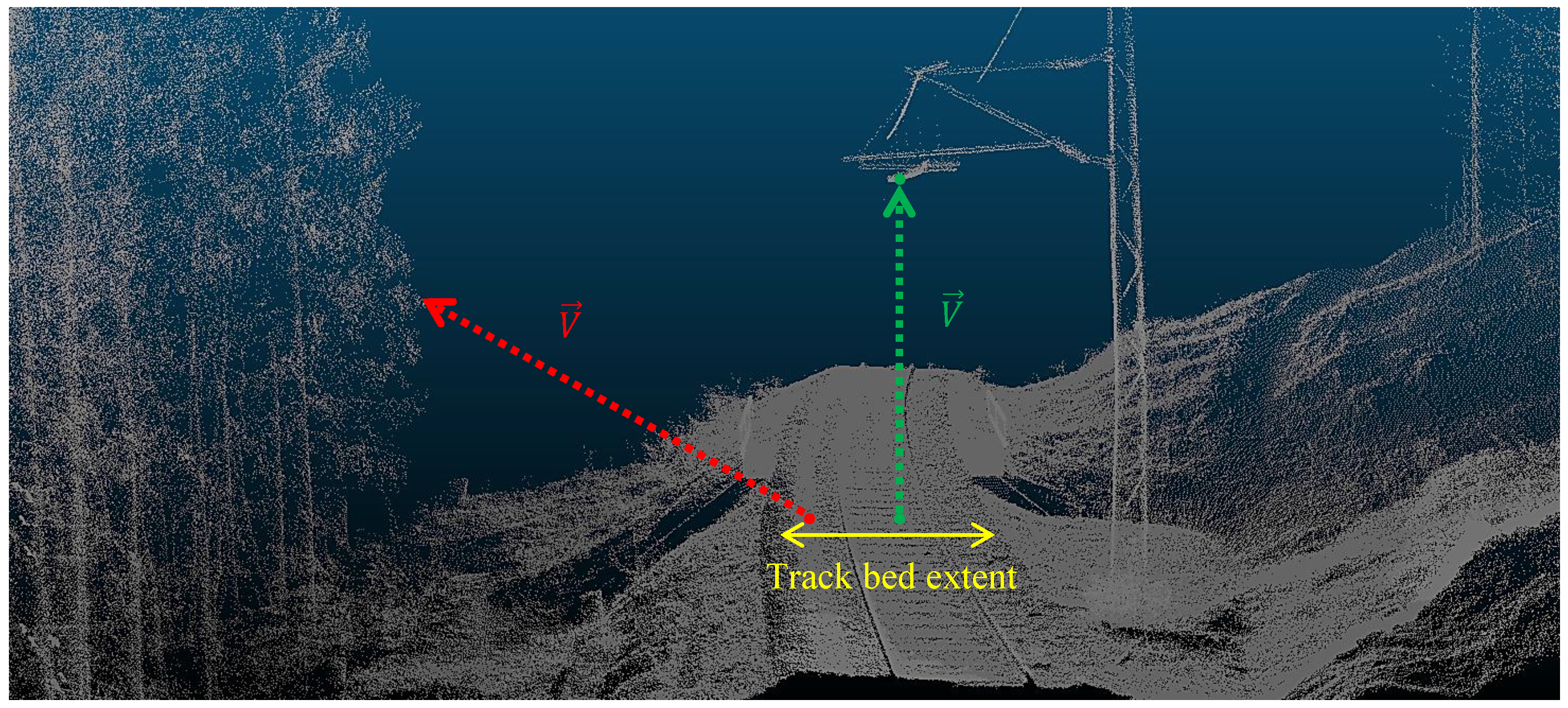
Overhead power cables lie within the areal extent of the track bed and in a certain height above it. First, the 3D vector connecting each non-track bed point to its closest point on the track bed is computed. If the vector is along vertical direction (as in Equation (2)), the non-track bed point is considered to lie above the track bed and is considered for subsequent processing.

$$n{V}_z\ge 0.8$$

(2)

where:

$$n{V}_i=\frac{V_i}{\sqrt{|V_x{|}^2+|V_y{|}^2+|V_z{|}^2}}(\text{Considering\hspace{0.17em}}\overrightarrow{V}=(V_x,V_y,V_z))$$

(3)

$n{V}_z$ is the normalized Z component of vector $\overrightarrow{V}$ and its value is between zero (representing a completely horizontal vector) and one (representing a completely vertical vector). The threshold in Equation (2) is selected according to the spatial offset among the track bed and overhead power cables. An ideal threshold includes only points belonging to cables and excludes other points, such as the ones belonging to surrounding environment. Herein, the priority is given to including all cable points at the expense of including some non-cable points, which can be eliminated in the next step. Equation (2) recognizes points belonging to cables, cantilevers, topmost part of the masts, and some surrounding vegetation as points lying above the track bed. These points are considered for further processing to recognize cables, cantilevers, and masts. Figure 8 indicates a sample part of data in which a point belonging to a cable is connected to its closes point on the track bed by a vertical green dashed arrow while another point belonging to the surrounding environment is connected to its closest point on the track bed with a non-vertical red dashed arrow.

Figure 8. A point above the track bed and within its areal extent is connected to its closest point on the track bed by a vertical green dashed arrow. A point lying outside of the track bed areal extent is connected to its closest point on the track bed by a non-vertical red dashed arrow.

Figure 8. A point above the track bed and within its areal extent is connected to its closest point on the track bed by a vertical green dashed arrow. A point lying outside of the track bed areal extent is connected to its closest point on the track bed by a non-vertical red dashed arrow.

Contact cables appear as straight linear objects while catenary and return current cables appear as curvilinear-shaped objects. Thus, all points identified as lying above the track bed are inspected to find the ones belonging to linear neighbourhood. To this end, three-dimensional PCA is employed by eigenvalue decomposition of the covariance matrix of local neighbourhoods. First, the covariance matrix of local neighbourhoods above the track bed is constructed. Then, eigenvalues of each covariance matrix are computed as follows:

$$\sum V=\lambda V\Rightarrow (\sum -\lambda I)V=0$$

(4)

$$\text{det}(\sum -\lambda I)=0$$

(5)

where Σ: Square 3 × 3 covariance matrix of a local neighbourhood; λ: Scalar eigenvalue; V: 3 × 1 matrix representing an eigenvector ($\overrightarrow{\nu }$) i.e., $V={\left(\begin{array}{ccc}{V}_x& V_y& V_z\end{array}\right)}^T$ and $\overrightarrow{\nu }=\left(V_x,V_y,V_z\right)$; I: Square 3 × 3 identity matrix

Solving Equation (5) results in three (scalar) eigenvalues (${\lambda }_1,{\lambda }_2,{\lambda }_3$; assuming ${\lambda }_1\ge {\lambda }_2\ge {\lambda }_3$). Each eigenvalue (${\lambda }_i$) is then used in Equation (4) to compute its corresponding eigenvector (${\overrightarrow{\nu }}_i$). As a result, three eigenvectors (${\overrightarrow{\nu }}_1,{\overrightarrow{\nu }}_2,{\overrightarrow{\nu }}_3$) are computed. If the following condition is met, the point under study is considered to have a linear neighbourhood and, thus, is considered as a candidate point for belonging to a contact cable:

$$n{\lambda }_1\approx 1andn{\lambda }_2\approx n{\lambda }_3\approx 0$$

(6)

where:

$$n{\lambda }_i=\frac{{\lambda }_i}{{\displaystyle \sum _{j=1}^3{\lambda }_j}}(n{\lambda }_i:{\text{i}}^{\text{th}}\text{ normalized eigenvalue})$$

(7)

Details of PCA and its applications to identify linear patterns in 3D LIDAR data can be found in [31,32], where it is detailed why Equation (6) identifies linear neighbourhoods. Points identified as belonging to a linear neighbourhood include points on contact cables, catenary cables, and return current cables. Thus, they are further processed to identify the points belonging to contact cables and also aggregate them in one segment. To this end, a region growing algorithm is employed. Points identified as belonging to a linear neighbourhood (by the condition in Equation (6)) are considered as seed points. The algorithm starts by randomly choosing a seed point (let us call it $P_{seed}$) and clustering points within 20-cm 3D Euclidean distance of the seed point. The similarity measures for clustering are two following criteria:

$$|H_{P_{seed}}-H_{P_{candidate}}|\le 20cm$$

(8)

$$\alpha \le {20}^{\circ }$$

(9)

where:

$$\alpha =\arcsin (\frac{{\overrightarrow{V}}_{P_{seed}}\times {\overrightarrow{V}}_{P_{candidate}}}{\left|{\overrightarrow{V}}_{P_{seed}}\right|\left|{\overrightarrow{V}}_{P_{candidate}}\right|})$$

(10)

The criterion in Equation (8) checks whether the height of the candidate point is approximately the same as the height of the seed point. The condition in Equation (9) tests if the linear neighbourhoods of the candidate and seed point are parallel. The height and angle thresholds in Equations (8) and (9) are derived from the physical shapes of overhead cables. Contact cables (as straight linear objects) do not have a large height variation (greater than 20 cm) or an abrupt change in their direction vector (greater than 20°) within a 20-cm 3D spherical neighbourhood. However, catenary cables and return current cables do experience such a height variation and direction vector change in such a small neighbourhood due to their curved shape. As a result, points belonging to a contact cable are clustered in one segment while segmentation results of other two types of cables suffer from over-segmentation i.e., each catenary and return current cable is broken into many small linear segments. The length of each segment belonging to catenary or return current cable does not exceed one meter, considering the curved shape of these cables. Therefore, once the length of a linear segment exceeds one meter, it is considered as belonging to a contact cable and the height and direction vector of query points are compared with those of most recently-clustered points (let us call them “edge points”) of the segment rather than the seed point’s height and direction vector. This way, the height and direction vector of the growing segment is updated as it grows.

Figure 9a demonstrates a side view of a growing contact cable segment in which the segmented points are shown by green color and the edge points are indicated by blue color. In this figure, a query point (orange point) is shown that is at the same height as the growing segment’s edge points (blue points), whereas catenary points (red points) lie higher than the growing segment and, thus, are not clustered. Furthermore, red arrows show that the local direction vectors along a catenary cable change (due to their curved shape) that result in over-segmentation. Figure 9b indicates the plan view of the growing segment, which is colorized with the same color scheme as Figure 9a. In this figure, the blue arrow indicates the direction vector of the edge points, the orange arrow points to the direction vector of the query point on a contact cable and the red arrow represents the direction vector of the query point on a mast or a cantilever. The orange point, in this example, is in the line with the edge points and, thus, is clustered in the growing segment while the direction vector of red points makes a large angle with the direction vector of edge points and, thus, red points are not clustered.

Figure 9. (a) A growing contact cable segment is depicted in a side view in which catenary cable points are not clustered due to their height difference. Arrows indicate local direction vectors; (b) The growing segment is indicated in a plan view in which points on mast and cantilevers (red points) are not clustered since they are not in line with the growing segment.

Figure 9. (a) A growing contact cable segment is depicted in a side view in which catenary cable points are not clustered due to their height difference. Arrows indicate local direction vectors; (b) The growing segment is indicated in a plan view in which points on mast and cantilevers (red points) are not clustered since they are not in line with the growing segment.

Catenary cables lie immediately above the contact cables. Thus, the 3D vector connecting each point above the track bed to its closest point on a contact cable is computed. If this vector is vertically distributed (as in Equation (2)), the point under study is considered as belonging to a catenary cable. Afterwards, all points that belong to catenary cables and are in 20-cm 3D Euclidean distance of one another are clustered. Figure 10 displays the location and spatial offset among a catenary cable, a return current cable, and a contact cable.

Return current cables also appear as curvilinear-shaped objects lying highest among objects above the track bed. Thus, points with linear neighbourhoods that lie above the catenary cables are considered as belonging to return current cables. Linear neighbourhoods are recognized by employing eigenvalue analysis as in Equations (4)–(6). The return current cable points that are in 20-cm 3D Euclidean distance of one another are clustered. Since droppers lie between contact and catenary cables, they are almost entirely occluded, which make their recognition not feasible.

Figure 10. Vectors connecting points on a catenary cable to a contact cable (green arrows) are vertical, while vectors connecting other objects to a contact cable (red arrows) are not vertical.

Figure 10. Vectors connecting points on a catenary cable to a contact cable (green arrows) are vertical, while vectors connecting other objects to a contact cable (red arrows) are not vertical.

3.5. Recognition of Masts and Cantilevers

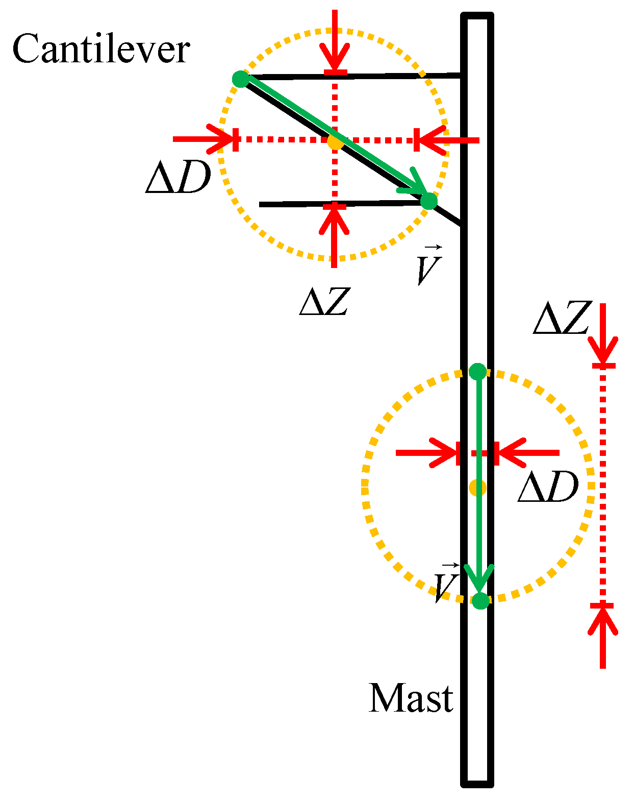
Objects above the track bed consist of overhead power cables, masts, and cantilevers. Overhead power cables are recognized in the previous section. Thus, the remaining points above the track bed are identified as belonging to masts and cantilevers. However, they cover only parts of the masts lying above the track bed. Therefore, a region-growing algorithm is utilized to identify the not-recognized points on masts. To this end, the non-cable points above the track bed are considered as seed points. The algorithm randomly selects a seed point and clusters un-segmented (non-cable) points in 20-cm 3D Euclidean distance of the seed point until it reaches to the local height of the track bed. Each resulting segment contains both a mast and a cantilever, which need to be separated. Masts are vertically distributed objects while cantilevers are distributed along both horizontal and vertical directions. This is evident in Figure 11 in which vertical distribution of a point on a mast and 3D distribution of a point on a cantilever is depicted. To separate the masts from cantilevers in each segment, one-meter 3D spherical neighbourhood of each and every point is investigated and once the following two conditions are satisfied, the point under inspection is considered as belonging to a mast. Otherwise, it is considered to belong to a cantilever.

Figure 11. In contrast to points on cantilevers, neighbourhoods of points on masts are vertically distributed. Orange points and circles represent query points and their 3D spherical neighbourhood:

Figure 11. In contrast to points on cantilevers, neighbourhoods of points on masts are vertically distributed. Orange points and circles represent query points and their 3D spherical neighbourhood:

$$\Delta D\le 20cm$$

(11)

$$n{V}_z\ge 0.8$$

(12)

where $\Delta D$ denotes a neighbourhood extent along horizontal direction and $n{V}_z$ is the normalized Z component of $\overrightarrow{V}$, which connects two farthest points in each neighbourhood. Equation (11) checks if a query neighbourhood is vertically distributed and Equation (12) tests if the vector connecting the two farthest points in each neighbourhood is also vertically distributed. Thresholds in Equations (11) and (12) are selected based on the planimetric dimension of masts that is roughly 20 cm. As a result, points on masts and cantilevers are separated and clustered into different segments.

4. Dataset

The dataset used in this study is acquired by an Optech Lynx mobile mapping system, shown in Figure 12. The imaging unit of this mobile mapper is composed of two 360° field of view laser scanners, two high-resolution cameras, and/or one 360° field of view camera. The navigation unit of the mobile mapping system includes an integrated GNSS/INS system. Table 1 presents the detailed specifications of this mobile mapping system.

Figure 12. An Optech Lynx mobile mapping system [33].

Figure 12. An Optech Lynx mobile mapping system [33].

Table 1. Specifications of Optech Lynx, the mobile mapper used to collect data in this research.

Parameters	Values
Measurement rate	Up to 1.2 million points per second
Range precision	5 mm
Positional accuracy	5 cm
Maximum range	250 m

Table 1. Specifications of Optech Lynx, the mobile mapper used to collect data in this research.

Parameters	Values
Measurement rate	Up to 1.2 million points per second
Range precision	5 mm
Positional accuracy	5 cm
Maximum range	250 m

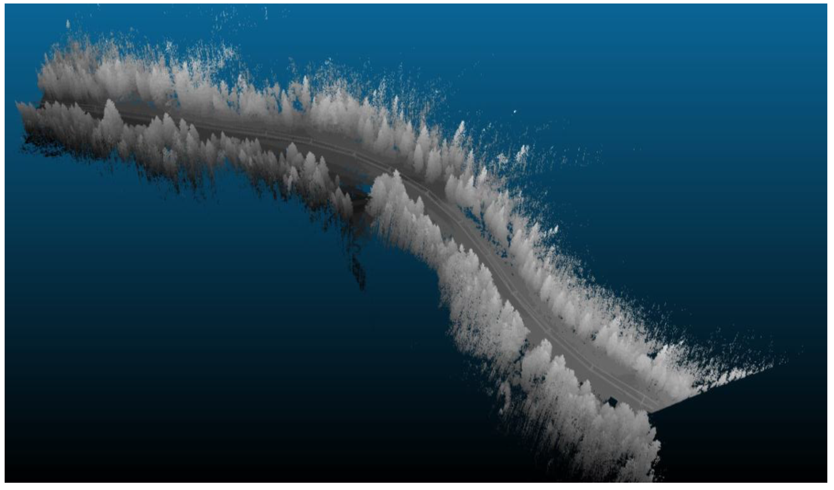
The mobile mapper was mounted on a car and placed on an open-top railcar operating at 125 km/h to avoid interference with the regular train schedule. The collected dataset contains more than 12.5 million points covering about 550 meters of Austrian railroads. The planimetric size of the area is 592 m × 322 m, with 73 m height variation. Figure 13 demonstrates the entire dataset from an oblique view and Figure 14 provides a close-up view of a portion of the dataset. The grey-scale colorization of these two figures is only to provide a decent visualization. The dataset contains only spatial information i.e., 3D co-ordinates of points with no intensity data and no RGB data of the integrated digital cameras. It covers points on railroad infrastructure i.e., track bed, rail tracks, overhead power cables, masts, cantilevers, as well as the surrounding environment, such as the terrain, trees, etc.

Figure 13. LIDAR dataset of Austrian railroad corridor, scanned by an Optech Lynx mobile mapping system.

Figure 13. LIDAR dataset of Austrian railroad corridor, scanned by an Optech Lynx mobile mapping system.

Figure 14. A close-up view of Austrian railroad infrastructure.

Figure 14. A close-up view of Austrian railroad infrastructure.

As is evident in Table 1, the scanner’s high range precision (5 mm) and high positional accuracy (5 cm) propose high quality data in which the noise level of the dataset is quite minimal. The dataset is not cleaned for noise removal and the entire acquired dataset is employed for processing. The point sampling on railroad components in this dataset is presented in Table 2. Various components have different point sampling due to their different dimensions and spatial offset from the LIDAR sensors. Contact and catenary cables have roughly similar point sampling since they are of the same dimensions and almost in the same spatial offset from the scanners. Return current cables have the lowest point sampling due to their thin structure and farther distance from the scanners, compared to other cables. Although masts are distributed along both horizontal and vertical directions, their vertical dimension (height) is much larger than their planimetric dimension. Thus, their point sampling is inspected as the number of points in one meter along vertical direction. Cantilevers are Z-shaped objects composed of three poles whose top pole is usually poorly-sampled due to occlusion (about 15 points/m). Table 2 provides the point sampling of the bottom and the diagonal poles of cantilevers.

Table 2. Point sampling on various components of railroad infrastructure.

Object	Point Sampling
Track bed (around rail tracks)	900 points/m2
Contact cable	28 points/m
Catenary cable	21 points/m
Return current cable	10 points/m
Mast	225 points/m
Cantilever	55 points/m

Table 2. Point sampling on various components of railroad infrastructure.

Object	Point Sampling
Track bed (around rail tracks)	900 points/m2
Contact cable	28 points/m
Catenary cable	21 points/m
Return current cable	10 points/m
Mast	225 points/m
Cantilever	55 points/m

5. Results and Discussion

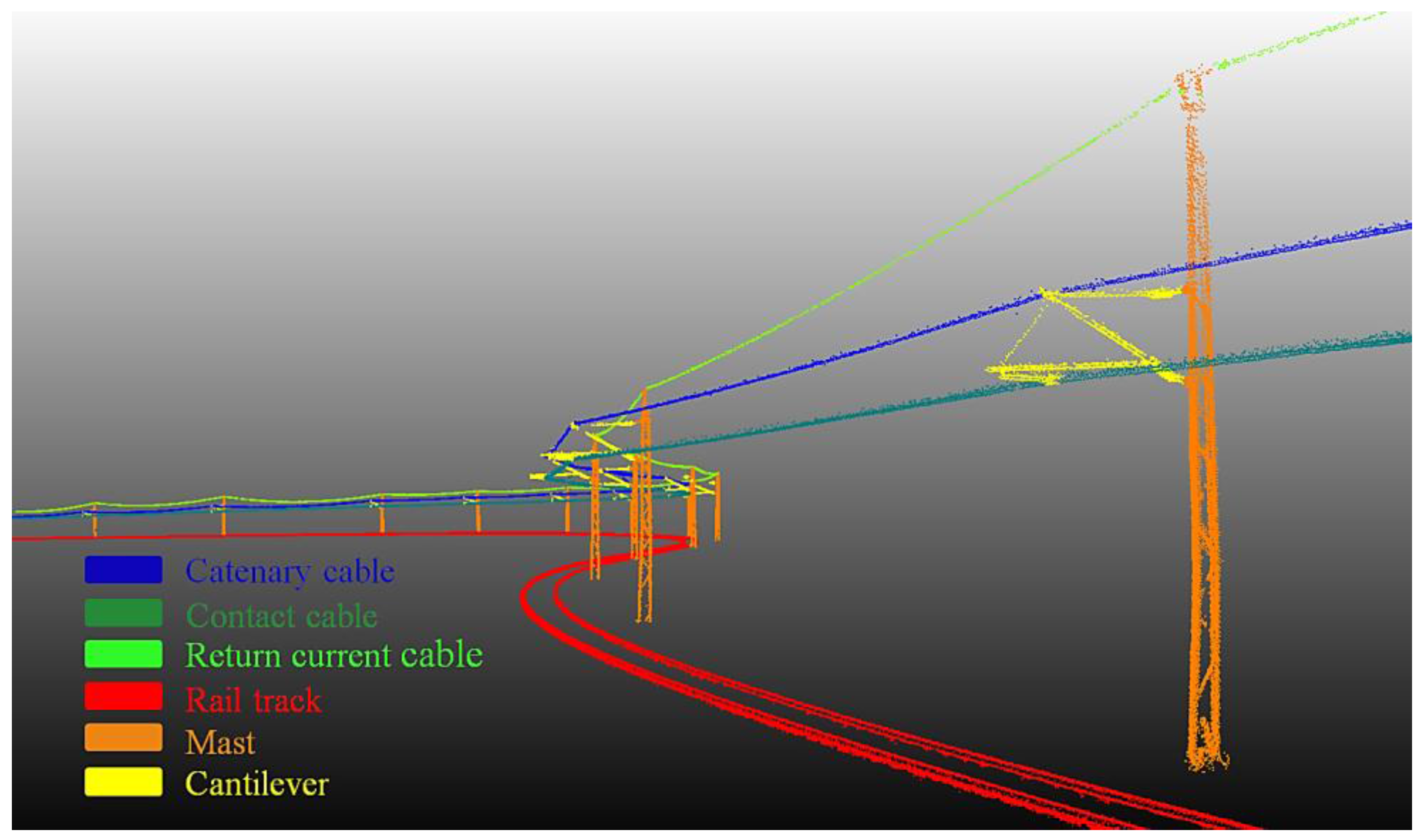
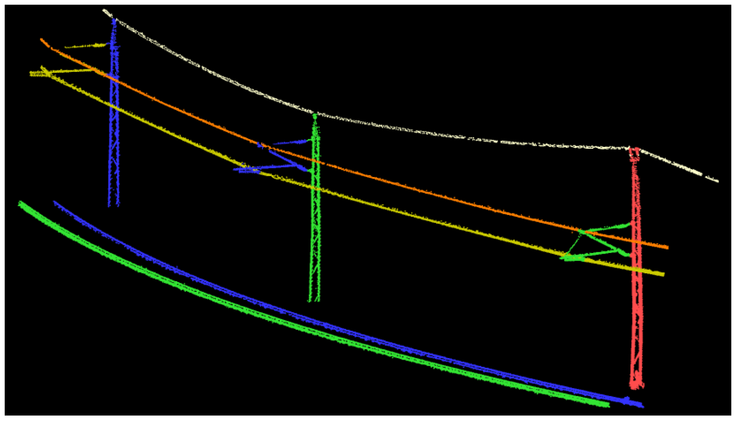
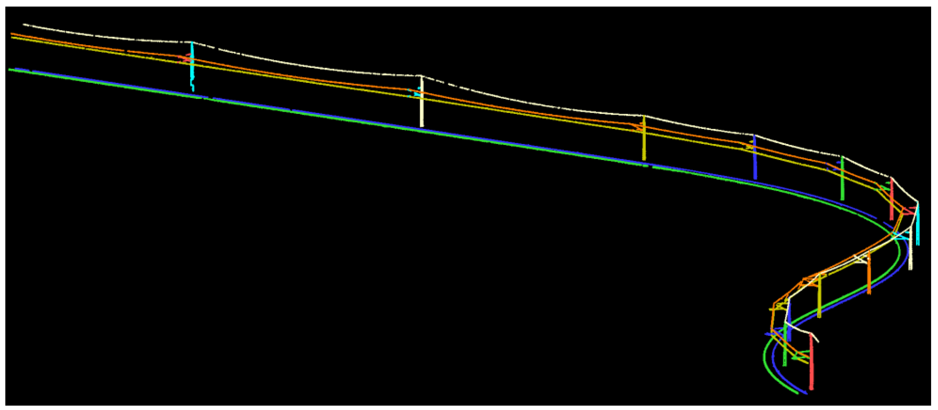
Figure 15 portrays the recognized railroad infrastructure, which is color-coded according to objects’ type. Figure 16 and Figure 17 visualize the recognized railroad components in which each color represents a separate object, regardless of its type.

Figure 15. Recognized railroad infrastructure. The figure is colorized according to objects’ type i.e., different object types are indicated by different colors.

Figure 15. Recognized railroad infrastructure. The figure is colorized according to objects’ type i.e., different object types are indicated by different colors.

Figure 16. Recognized railroad key components (regardless of their types) are visualized by different colors.

Figure 16. Recognized railroad key components (regardless of their types) are visualized by different colors.

Figure 17. A close-up view of the recognized railroad key elements. Each color represents a separate object, regardless of its type.

Figure 17. A close-up view of the recognized railroad key elements. Each color represents a separate object, regardless of its type.

The achieved results are assessed by manual delineation of the objects of interest. The assessment is carried out both at object level and at point cloud level. Table 3 presents the recognition results at object level indicating that all key components of railroad corridors are successfully recognized with no false positives and no false negatives. This corresponds to 100% precision and 100% accuracy at the object level. Precision and accuracy are computed as follows:

$$\text{Precision\hspace{0.17em}}=\frac{tp}{tp+fp}$$

(13)

$$\text{Accuracy\hspace{0.17em}}=\frac{tp+tn}{tp+tn+fp+fn}$$

(14)

where $tp$, $tn$, $fp,$ and $fn$ denote true positive, true negative, false positive, and false negative, respectively.

Table 3. Results at object level in terms of the number of recognized objects.

Object Type	Number of Objects in Data	True Positives	True Negatives	False Positives	False Negatives
Rail track	2	2	29	0	0
Contact cable	1	1	30	0	0
Catenary cable	1	1	30	0	0
Return current	1	1	30	0	0
Mast	13	13	18	0	0
Cantilever	13	13	18	0	0
All objects	31	31	NA	0	0

Table 3. Results at object level in terms of the number of recognized objects.

Object Type	Number of Objects in Data	True Positives	True Negatives	False Positives	False Negatives
Rail track	2	2	29	0	0
Contact cable	1	1	30	0	0
Catenary cable	1	1	30	0	0
Return current	1	1	30	0	0
Mast	13	13	18	0	0
Cantilever	13	13	18	0	0
All objects	31	31	NA	0	0

Table 4 demonstrates the recognition results at point cloud level in terms of accuracy and precision, which are computed as in Equations (13) and (14). Achieved results depict that overall average 96.4% recognition accuracy is obtained. While masts and rail tracks have the highest recognition accuracy (greater than 98%), cantilevers have the lowest accuracy (91%) among all railroad corridor components. In addition, overhead power cables reached an average of 96.43% recognition accuracy.

Table 4. Results at point cloud level in terms of recognition accuracy and precision.

Object	Accuracy (in Percentage)	Precision (in Percentage)
Rail tracks	98.34	98.47
Contact cable	97.66	96.02
Catenary cable	96.92	95.87
Return current cable	94.72	99.63
Masts	99.42	95.17
Cantilevers	91.23	97.43
Average	96.4	97.1

Table 4. Results at point cloud level in terms of recognition accuracy and precision.

Object	Accuracy (in Percentage)	Precision (in Percentage)
Rail tracks	98.34	98.47
Contact cable	97.66	96.02
Catenary cable	96.92	95.87
Return current cable	94.72	99.63
Masts	99.42	95.17
Cantilevers	91.23	97.43
Average	96.4	97.1

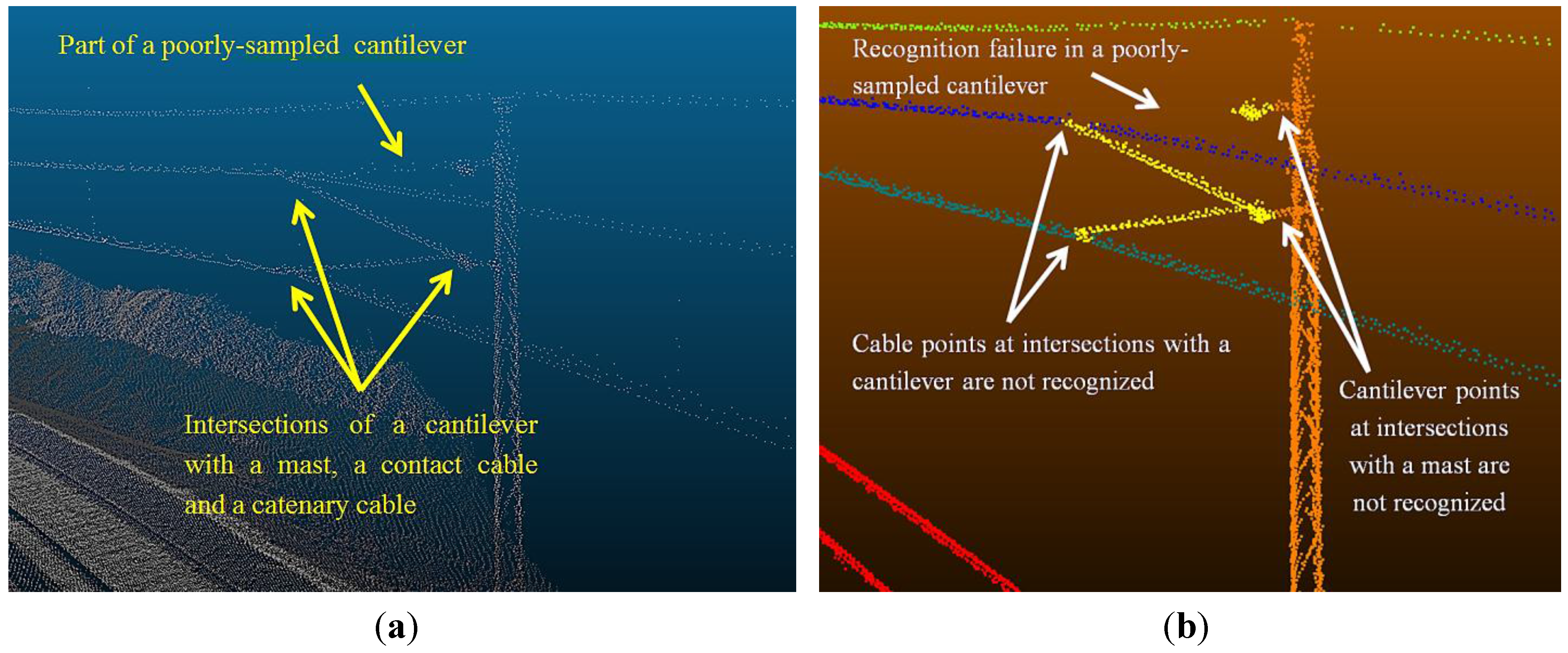
Poor sampling (low point spacing), occlusions, and object intersections are three primary causes of non-perfect recognition. Poor sampling profoundly deteriorates object recognition results. The developed algorithm is not able to fully recognize the poorly-sampled objects since they do not provide sufficient amount of information required for their recognition. This is reflected in the recognition accuracy of the return current cable that is the lowest among all types of cables, provided that return current cable has the lowest point sampling among all objects. Figure 18a indicates a poorly-sampled part of a cantilever and some intersections of objects and Figure 18b depicts the recognition failure in the very same parts.

Figure 18. (a) Some instances of poor sampling, occlusion, and object intersection in the dataset; (b) Object recognition results in the very same areas.

Figure 18. (a) Some instances of poor sampling, occlusion, and object intersection in the dataset; (b) Object recognition results in the very same areas.

Low point spacing can be due to the far distance of the objects from the scanner, small dimensions of an object or occlusion. Occlusion is the shadow effect that occurs once an object blocks a laser beam and prevents it from reaching to another object. Due to the railroad corridors configuration, some objects might be occluded e.g., catenary cables lie immediately above contact cables and are partially occluded. The largest occlusions, however, occur to cantilevers that are located among three objects (i.e., masts, contact cables, and catenary cables) and as a result, they have the lowest recognition accuracy among all objects. Furthermore, the developed algorithm fails at the intersection of objects where the local neighbourhood reflects a structure that is similar to none of the objects at the intersection. The high recognition accuracy of well-sampled objects highlights the negative impact of occlusion and poor sampling on recognition results.

False positives at the point cloud level are presented in Table 4 as recognition accuracy and precision. Rail track false positives occur due to height variations introduced by non-rail objects, such as external objects and vegetation on the track bed. The region growing algorithm employed in rail track recognition filtered out many height variations caused by non-rail objects. However, the ones that are not eliminated are located quite close to rail tracks. Recognition precision of contact cables, catenary cables, and masts are very close to one another since their false positives took place only at their intersections with cantilevers. High precision of cantilevers implies that the recognized cantilevers contain very few false positives. Return current cables have the highest precision, which is primarily due to its (curvilinear) shape and distinctive topology i.e., it is intersected only with masts in rather long spatial intervals. As a result, there are very few false positives in the recognized return current cable.

Thresholds used in this work are derived from approximate dimensions of objects, spatial offset, and topological relationships among objects. In the recognition of each type of object, some thresholds are automatically determined and some are manually determined. For instance, in the track bed and rail track recognition, height standard deviation of points belonging to the track bed and rail tracks are automatically determined by the developed algorithms. Table 5 presents the types, values, and rationale of manually-determined thresholds in which angle and distance thresholds refer to thresholds employed in the region growing algorithms and vector verticality refers to normalized Z component of a query vector.

Table 5. Types and rationale of thresholds used in this work.

Object	Threshold Type	Threshold Value	Rationale
Rail track	Angle threshold	20°	Tracks smooth curvature gradient
	Distance threshold	1 m	Track gauge
Contact cable	Vector verticality	0.8	Railroad corridor configuration
	Angle threshold	20°	Tracks smooth curvature gradient
	Height variation	20 cm	Contact cables straight linear shape
Catenary cable	Vector verticality	0.8	Railroad corridor configuration
Mast	Vector verticality	0.8	Railroad corridor configuration
	Planimetric extent	20 cm	Masts physical shape

Table 5. Types and rationale of thresholds used in this work.

Object	Threshold Type	Threshold Value	Rationale
Rail track	Angle threshold	20°	Tracks smooth curvature gradient
	Distance threshold	1 m	Track gauge
Contact cable	Vector verticality	0.8	Railroad corridor configuration
	Angle threshold	20°	Tracks smooth curvature gradient
	Height variation	20 cm	Contact cables straight linear shape
Catenary cable	Vector verticality	0.8	Railroad corridor configuration
Mast	Vector verticality	0.8	Railroad corridor configuration
	Planimetric extent	20 cm	Masts physical shape

Neighbourhood size is selected in a way to provide reliable information about physical characteristics of an object without including points belonging to other objects. The 20-cm neighbourhood size, which is used in the majority of algorithm steps, provides such reliable information. In track bed recognition and in the last step of masts and cantilevers recognition, one meter neighbourhood size is used, considering the large dimensions of the track bed and masts. Furthermore, specific region-growing algorithms are developed in various parts of methodology to cluster the classified points. The clustering distance threshold in all parts of the methodology is 20 cm, considering topological relationships among objects.

6. Conclusions

This paper proposes a novel methodology for fully-automated recognition of railroad corridor key elements using 3D LIDAR data. Key components of railroad corridors are rail tracks, contact cables, catenary cables, return current cables, masts, and cantilevers. The data was acquired by an Optech Lynx mobile mapping system, which was mounted on a railcar operating at 125 km/h. The dataset covers 550 m of Austrian rural railroad corridor. The proposed methodology achieved 100% accuracy and 100% precision at the object level, implying that all objects of interest, including two rail tracks, thirteen masts, thirteen cantilevers, one contact cable, one catenary cable, and one return current cable were successfully recognized. Furthermore, an average of 96.4% accuracy and an average of 97.1% precision at the point cloud level were obtained. Analysis of the results indicates that poor sampling, occlusions, and object intersections are three primary causes of non-perfect recognition at the point cloud level. The achieved results provide an accurate and precise representation of the current state of the railroad infrastructure.

7. Outlook

This study can be pursued to construct as-built 3D models of railroad corridors. Although the achieved results are sufficient for the intended purposes of this work (safety, maintenance, and future design enhancements), 3D models can provide a more user-friendly environment. To this end, as-built 3D models can be constructed by fitting 3D CAD models to the recognized railroad components.