1. Introduction
CORINE land cover mapping provides the only consistent classification system of long-term land cover data in Europe [
1]. With its 44 classes, some of which are defined as mixed land cover and land use classes, CORINE provides a European scale map with 25 ha minimum mapping unit for land cover and 5 ha for land cover change every 6 years [
2].
CORINE land cover maps are important as a source of operational land cover information for many sectors of the European economy, including risk management for the insurance industry [
3], telecommunications planning, environmental reporting, land use impact assessment on the natural environment [
4], life cycle analysis [
5], biodiversity and habitat conservation [
6], population distribution mapping [
7], crop forecasting [
8], urban heat island studies [
9] and others.
Historically, member states of the European Environment Agency have adopted national approaches for the production of CORINE; with many choosing to follow the Agency’s published Technical Guidelines [
10]. These guidelines foresee a manual digitization of land cover change based on visual interpretation of optical/near-infrared satellite images. This process is both subjective to some extent, even with the internal and external quality assurance and verification steps that are compulsory, and labour intensive. In the current CORINE mapping process to produce a 2012 map, frequent cloud cover has made the provision of optical imagery over the British Isles and parts of Scandinavia very patchy and difficult to fulfil within the specified user requirements.
SAR is an active imaging technique that is not hampered by frequent cloud-cover because microwave radiation penetrates through clouds. The European Space Agency (ESA) has launched the first of its Copernicus Sentinel missions in April 2014. Sentinel-1A provides C-band SAR data in four acquisition modes with a temporal revisit time of 12 days with the first satellite and 6 days once Sentinel-1B has been launched in 2016 [
11]. The acquisition modes are Stripmap (SM), Interferometric Wide-Swath (IW), Extra Wide Swath (EW) and Wave Mode (WV). The SM, IW, and EW modes acquire data at a single transmit polarisation (H or V) and dual receive polarisation (HV or VH). The WV mode only has a single polarisation (HH or VV). The default mode over land is the Interferometric Wide-Swath Mode, which provides a 250 km swath composed of three sub-swaths at 5 m by 20 m spatial resolution in single look. It uses a new type of ScanSAR mode called Terrain Observation with Progressive Scan (TOPS) SAR, which is shrinking the azimuth antenna pattern along track direction.
Several studies have investigated the suitability of SAR for land cover mapping, but few have aimed at the delineation of a large number of classes, and fewer still have analysed C-band SAR data [
12]. Microwave radiation responds to fundamental scattering processes that are determined by surface roughness, soil moisture, vegetation water content and 3D structure of the scattering elements. A C-band SAR-based land cover classification of Kuwait showed a total of 13 classes could be distinguished from ERS-1/2 and Radarsat images [
13]. Vegetation cover, surface roughness, percentage of coarse material in the surface layer and moisture conditions influenced the backscatter. Most SAR classification algorithms use fixed polarimetric indices to detect certain land cover types, despite the large natural variability between observation sites, temporal acquisition, environmental conditions and calibration effects. To improve on previous approaches, a decision-tree-based adaptive land cover classification technique has been developed [
14].
The potential of Sentinel-1 for land cover mapping [
15] was recognised in a study that simulated the planned short revisit and dual-polarization concept of Sentinel-1 with multi-temporal ERS-2 and ENVISAT ASAR AP C-band backscatter data [
16]. Five basic level 2 land cover classes could be mapped consistently and operationally with accuracies greater than 85% covering 75,000 km
2 of Belgium, the Netherlands and Germany [
16]. C-band SAR backscatter is able to map burnt peat land as was shown for the CORINE peat bog class [
17]. Multitemporal/multi-polarization ENVISAT ASAR C-band data were investigated for principal component analysis and classification of five land cover classes in Korea [
18]. Sentinel-1 will provide IW mode acquisitions over land areas, making it suitable for SAR interferometry (InSAR), which offers the retrieval of canopy height models and digital terrain models from SAR and is particularly promising for forest mapping [
19]. Interferometric coherence also discriminates between forest growing stock volume classes [
20].
Some studies cast doubts on the ability of SAR to map land cover with acceptable accuracy. ALOS PALSAR L-band and RADARSAT-2 C-band data were tested for land cover classification in a moist tropical region [
21]. L-band provided 72.2% classification accuracy for a coarse land cover classification system (forest, succession, agro-pasture, water, wetland, and urban) and C-band only 54.7%.
An important feature of SAR images is their image texture, which can be quantified by a range of different statistical measures that are calculated over a moving window of specific size. For example, ALOS PALSAR 50 m FBD data were used to map land cover in Riau province, Sumatra, Indonesia [
22]. The radiometric information in the L-band HH and HV channels alone was a poor classifier, and textural parameters were needed to achieve land cover class discrimination. The SVM classifier in that study showed an agreement over 70% with six land cover classes derived from Landsat [
22]. Very high resolution TerraSAR-X data were used for land cover mapping by specifying the speckle characteristics of the land cover classes: water; open land (farmland, grassland, bare soil); woodland; and urban area, showing overall accuracies of 77%–86% [
23]. A combination of radiometric image bands and texture bands also increased the classification accuracies [
21].
The multi-temporal capabilities of Sentinel-1 are likely to improve its classification accuracy for land cover applications. Riedel
et al. [
24] generated a land use map with 20 crop types of Northern Thuringia with 80.2% overall accuracy from ASAR time-series by including texture information which they retrieved from multi-temporal statistics. Another study used X-band SAR with eleven COSMO-SkyMed HH and HV images for land cover mapping over an agricultural area in Southern Australia [
25]. The temporal information improved the classification results, with an overall accuracy of ca. 82% for 10 classes [
25]. Five land use/land cover types (forests, urban infrastructure, surface water and marsh wetland) were mapped from multi-temporal polarimetric RADARSAT-2 imagery in North-eastern Ontario, Canada [
26]. Wetlands showed a seasonal increase in HH and HV backscatter intensity due to the growth of emergent vegetation over the summer but other classes showed little temporal variation in backscatter. Multi-temporal RADARSAT-2 polarimetric SAR data were used to discriminate high-density residential areas, low-density residential areas, industrial and commercial areas, construction sites, parks, golf courses, forests, pasture, water, and two types of agricultural crops using an object-based support vector machine and a rule-based approach (κ = 0.91) [
27]. In the Brazilian Pantanal, multi-temporal L-band ALOS/PALSAR and C-band RADARSAT-2 data gave an accuracy of 81% for the land cover types of forest, savanna, grasslands/agriculture, aquatic vegetation and open water [
28].
Knowledge-based models have been used to determine hierarchical decision rules to differentiate land cover classes [
29]. In the approach by Dobson
et al. [
29] the classifier produces two levels of classification, first a terrain differentiation into man-made features (urban), surfaces, short vegetation, and tall vegetation, followed by a level 2 differentiation of the tall vegetation class based on foliage and growth form of woody stems (excurrent, decurrent, and columnar tree architecture), leading to overall accuracies over 90% in northern Michigan. The knowledge-based SAR-based classification by Dobson
et al. [
29] was superior to unsupervised classification of multi-temporal AVHRR data. A dictionary- and rule-based model selection approach was developed in an adaptive contextual semi-supervised algorithm for multi-temporal RADARSAT-2 polarimetric SAR (PolSAR) data [
30]. The best overall classification accuracy it achieved was 89.99%.
The synergistic use of optical and SAR data improves classification accuracy. Five land cover classes in the Arctic tundra were mapped with dual-polarized TerraSAR-X (HH/VV), quad-polarized Radarsat-2 and Landsat 8 imagery [
31]. The overall accuracy increased if both SAR and optical data were used (71% unsupervised Landsat 8 and TerraSAR-X; 87% supervised Landsat 8 and Radarsat-2).
Hierarchical decision trees are appealing for land cover mapping but usually require an interpretation by the observer to set the branching rules. To avoid reliance on this a priori knowledge, ensemble classification methods that originate from machine learning are increasingly prominent in the recent literature. One such method is random forests, a machine learning supervised classifier developed by Breiman [
32]. Random forests often provide better land cover classification accuracies than for example the maximum likelihood approach [
33]. In Waske and Brown [
33], boosted decision trees and random forests were applied to multi-temporal C-band SAR data from different study sites and years. Random forests outperformed all other classifiers and reached nearly 84% overall accuracy in rural areas [
33]. Random forest classification has been applied to salt marsh vegetation mapping from quad-polarimetric airborne S- and X-band SAR, elevation and optical data [
34].
This comprehensive literature review shows that most studies have limited themselves to mapping around five land cover classes from SAR, with only a handful of studies expanding the classification scheme to include more classes. Besides, no published studies of real Sentinel-1 data for the mapping of land cover classes are in the public domain at the date this manuscript was written.
This paper examines what is achievable from summer and winter acquisitions of Sentinel-1A dual-polarisation SAR data aided by prior knowledge of past land cover and digital elevation data from the Shuttle Radar Topography Mission.
2. Materials and Methods
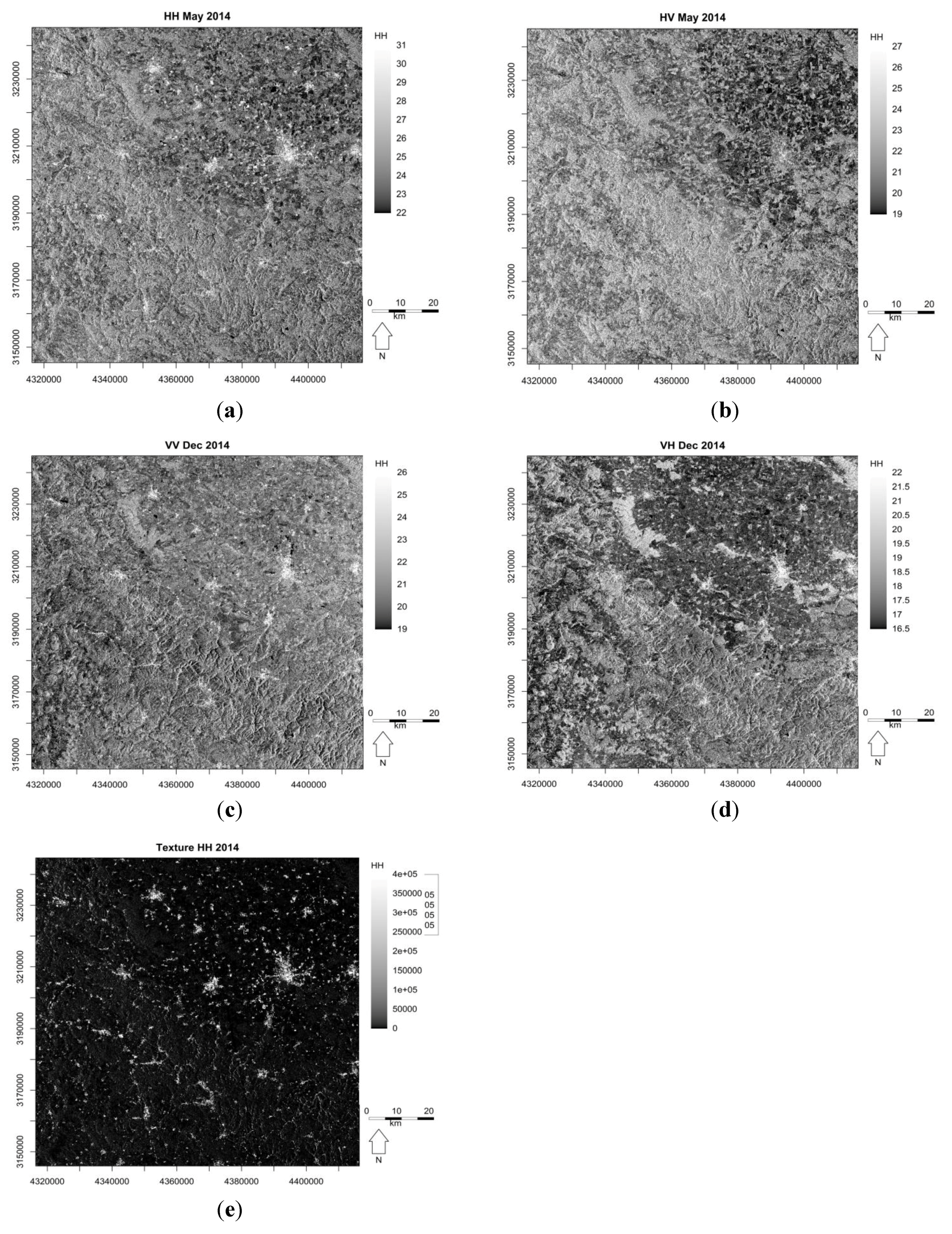
The present study analyses two of the first Sentinel-1A SAR image acquisitions over Thuringia, Germany. The first, uncalibrated Sentinel-1A image was acquired during the ramp-up phase on 2 May 2014 (Scene ID = S1A_IW_GRDH_1SDH_20140502T170314_20140502T170343_000421_0004CC), in ascending orbit at HH and HV polarisations. The second image was acquired on 9 December 2014 (Scene ID = S1A_IW_GRDH_1SDV_20141209T053327_20141209T053352_003638_0044F6), in descending orbit at VV and VH polarisations. Both images were processed to the Standard Level 1 Product, GRDH (ground-range detected, high resolution) by ESA. The images were not fully calibrated because during the Sentinel-1A ramp-up phase the calibration constants were not yet available from ESA, meaning that the backscatter values are not on an absolute scale. The backscatter bands contain Digital Numbers which are converted to the dB scale. The image bands are resampled to 100 m spatial resolution using bilinear interpolation. Texture bands are calculated from the GRDH image products within a moving 5 by 5 pixel window, calculating the variance within each window and them resampling to 100 m spatial resolution.
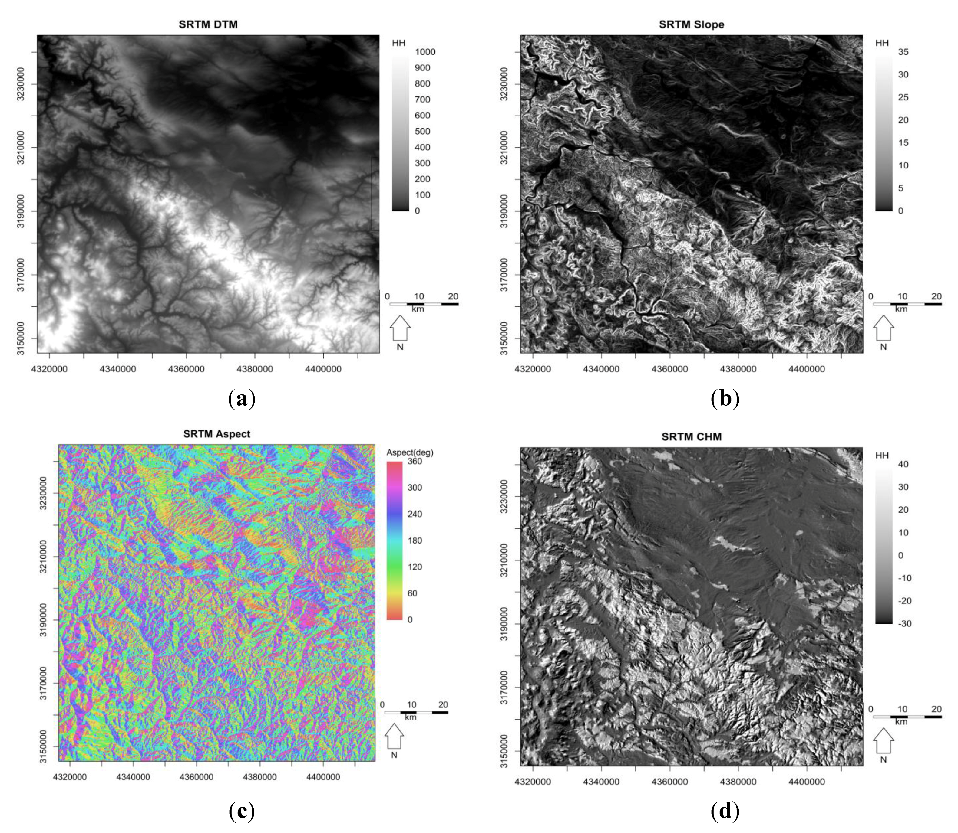
SRTM data [
35,
36,
37,
38] at 100 m spatial resolution were obtained from opentopography.org and SLOPE and ASPECT are calculated from the DTM in order to take into account the prevalence of certain land cover types on specific slopes, aspects or altitudes.
The 2006 CORINE land cover map for Germany was produced using the standard method of visual interpretation based upon the EEA technical guidelines [
10] and obtained as a gridded 100 m resolution product. A hybrid CORINE level 2/level 3 classification scheme of 27 classes is devised (
Table 1), based on knowledge of the scattering mechanisms of C-band SAR and the dependence of certain land cover types on geomorphology. All spatial data are resampled to the 100 m grid with a Lambert Azimuthal Equal Area projection (latitude at projection centre = 52°, longitude at projection centre = 10°, false easting = 4,321,000 m, false northing = 3,210,000 m, GRS80 ellipsoid, units = metre). The hybrid CORINE land cover map 2006 is used for the automatic extraction of pixels as training sites for the classifiers. To minimise edge effects, its polygons were first eroded by 5 pixels along the edges. Polygon erosion results were performed with different numbers of pixels (3, 5 and 7) and 5 pixels lead to eroded polygon areas that are sufficiently free of edge effects and location uncertainty effects from overlaying the CORINE polygon boundaries and the SAR viewing geometry. Up to 20,000 stratified random samples of training pixels are chosen for each CORINE class. A stratified random sampling approach is statistically appropriate for sampling distributions with highly imbalanced sample sizes such as often found in land cover datasets. We explored different caps of the number of training pixels and found that 20,000 was a good compromise between computational efficiency (because larger numbers increase the RF computation time) and coverage of representative areas of land cover types (which can be an issue if too few samples are used from land cover types with large area extent that become under-sampled and hence biased).
The processing of all datasets was implemented in R [
39], using the R packages “randomForest” [
40], “sp” [
41,
42], “caTools”, “gdalUtils”, “rgdal”, “foreign”, “raster”, “fields”, “rasclass” and “mmand”. Four random forest (RF) classifications are performed with different input bands to assess their relative performance:
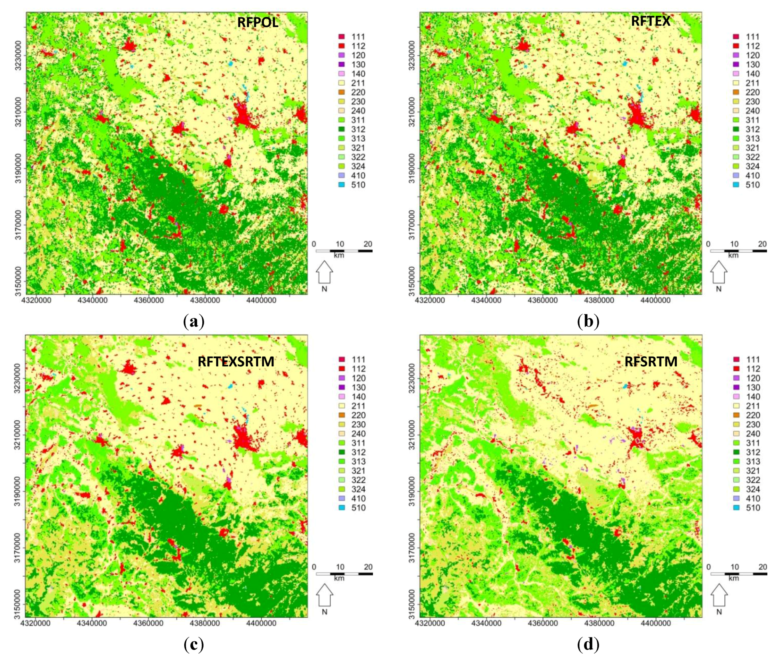
(i) RFPOL classification: A purely radiometric classification with HH and HV polarisations from May 2014 and VV and VH from December 2014.
(ii) RFTEX classification: Radiometric and texture information, with HH and HV polarisations from May 2014 and VV and VH from December 2014, as well as the HH texture band.
(iii) RFTEXSRTM classification: An integrated radiometric and texture classification with auxiliary geomorphometric input bands, using HH and HV polarisations from May 2014 and VV and VH from December 2014, the HH texture band, and the Digital Terrain Model (DTM), Canopy Height Model (CHM) and SLOPE and ASPECT maps from the Shuttle Radar Topography Mission (SRTM).
(iv) RFSRTM classification: A pure terrain classification using only the Digital Terrain Model (DTM), Canopy Height Model (CHM) and SLOPE and ASPECT maps from the Shuttle Radar Topography Mission (SRTM).
The principle of a random forest is the classification of the image layers by constructing a large number of decision trees [
32]. Random forests train classifiers to generate class predictions for unseen data. Randomness is introduced by bootstrapping and random selection of a subset of
m variables to split at each node of a tree. Splitting thresholds are defined using the Gini Index, which is a measure of the child node class homogeneity with respect to the distribution of classes in the parent node. Each object (either a pixel or a polygon) is classified as the class which gets the most “votes” from all the decision trees in the random forest. In the original implementation trees are grown to the largest possible size without pruning [
32].
Each of the RF classifiers used here generated 201 decision trees. All classifiers are post-processed with a 3 by 3 pixel local mode filter to remove isolated pixels and reduce noise in the land cover maps. The accuracy of the classified maps is assessed by calculating the out-of-bag error rates of the random forests for each CORINE class over the training pixels. The out-of-bag error rate is estimated internally by the random forest during the construction of each tree from a different bootstrap sample from the original data. One-third of the pixels (cases) are left out of the bootstrap sample for each tree and are then classified with that tree. A test classification of each pixel is obtained in this way from one-third of all trees. These independent test sets are used to estimate the out-of-bag error rate. It provides an unbiased estimate of the true map accuracy [
32].
Random forests allow the analysis of the variable importance with the Gini coefficient, which is a measure of the homogeneity of a distribution, ranging from 0 (completely homogeneous) to 1 (completely heterogeneous). The Gini coefficient originates from Economics where it is used to describe the inequalities of the distribution of wealth. In random forests, the Gini coefficient is calculated each time a particular input variable is used to split a node. The Gini coefficient for the child nodes are compared to that of the original node. If the split improves the homogeneity of classes, the Gini coefficient will decrease after splitting the node. All decreases in the Gini coefficient that are achieved for the nodes are added up for each input variable. Hence, input variables that result in nodes with higher classification purity have a higher decrease in Gini coefficient overall.
Table 1.
Description of the CORINE level 3 classification scheme with the original level 3 codes and the hybrid CORINE level 2/3 scheme used in this study with recoded class codes.
Table 1.
Description of the CORINE level 3 classification scheme with the original level 3 codes and the hybrid CORINE level 2/3 scheme used in this study with recoded class codes.
| Code | CORINE Level 3 | Recoded | Hybrid CORINE Level 2/3 |
|---|
| 111 | Continuous urban fabric | 111 | Continuous urban fabric |
| 112 | Discontinuous urban fabric | 112 | Discontinuous urban fabric |
| 121 | Industrial or commercial units | 120 | Industrial, commercial and transport units |
| 122 | Road and rail networks and associated land |
| 123 | Port areas |
| 124 | Airports |
| 131 | Mineral extraction sites | 130 | Mine, dump and construction sites |
| 132 | Dump sites |
| 133 | Construction sites |
| 141 | Green urban areas | 140 | Artificial, non-agricultural vegetated areas |
| 142 | Sport and leisure facilities |
| 211 | Non-irrigated arable land | 211 | Non-irrigated arable land |
| 212 | Permanently irrigated land | 212 | Permanently irrigated land |
| 213 | Rice fields | 213 | Rice fields |
| 221 | Vineyards | 220 | Permanent crops |
| 222 | Fruit trees and berry plantations |
| 223 | Olive groves |
| 231 | Pastures | 230 | Pastures |
| 241 | Annual crops associated with permanent crops | 240 | Heterogeneous agricultural areas |
| 242 | Complex cultivation patterns |
| 243 | Land principally occupied by agriculture, with significant areas of natural vegetation |
| 244 | Agro-forestry areas |
| 311 | Broad-leaved forest | 311 | Broad-leaved forest |
| 312 | Coniferous forest | 312 | Coniferous forest |
| 313 | Mixed forest | 313 | Mixed forest |
| 321 | Natural grasslands | 321 | Natural grasslands |
| 322 | Moors and heathland | 322 | Moors and heathland |
| 323 | Sclerophyllous vegetation | 323 | Sclerophyllous vegetation |
| 324 | Transitional woodland-shrub | 324 | Transitional woodland-shrub |
| 331 | Beaches, dunes, sands | 331 | Beaches, dunes, sands |
| 332 | Bare rocks | 332 | Bare rocks |
| 333 | Sparsely vegetated areas | 333 | Sparsely vegetated areas |
| 334 | Burnt areas | 334 | Burnt areas |
| 335 | Glaciers and perpetual snow | 335 | Glaciers and perpetual snow |
| 411 | Inland marshes | 410 | Inland wetlands |
| 412 | Peat bogs |
| 421 | Salt marshes | 420 | Maritime wetlands |
| 422 | Salines |
| 423 | Intertidal flats |
| 511 | Water courses | 510 | Inland waters |
| 512 | Water bodies |
| 521 | Coastal lagoons | 520 | Marine waters |
| 522 | Estuaries |
| 523 | Sea and ocean |
Table 2.
Number of pixels selected randomly for each hybrid CORINE level 2/3 class as training data for the classifiers.
Table 2.
Number of pixels selected randomly for each hybrid CORINE level 2/3 class as training data for the classifiers.
| Class | Description | Number of Pixels in the CLC 2006 Map | Number of Training Pixels |
|---|
| 111 | Continuous urban fabric | 543 | 119 |
| 112 | Discontinuous urban fabric | 50,613 | 8,832 |
| 120 | Industrial, commercial and transport units | 9,117 | 1,143 |
| 130 | Mine, dump and construction sites | 1,641 | 68 |
| 140 | Artificial, non-agricultural vegetated areas | 3,574 | 271 |
| 211 | Non-irrigated arable land | 431,518 | 20,000 |
| 220 | Permanent crops | 1,915 | 395 |
| 230 | Pastures | 80,113 | 14,972 |
| 240 | Heterogeneous agricultural areas | 38,663 | 6,549 |
| 311 | Broad-leaved forest | 102,895 | 20,000 |
| 312 | Coniferous forest | 202,476 | 20,000 |
| 313 | Mixed forest | 58,720 | 13,473 |
| 321 | Natural grasslands | 11,356 | 5,145 |
| 322 | Moors and heathland | 247 | 12 |
| 324 | Transitional woodland-shrub | 1,431 | 132 |
| 410 | Inland wetlands | 395 | 32 |
| 510 | Inland waters | 2,748 | 334 |
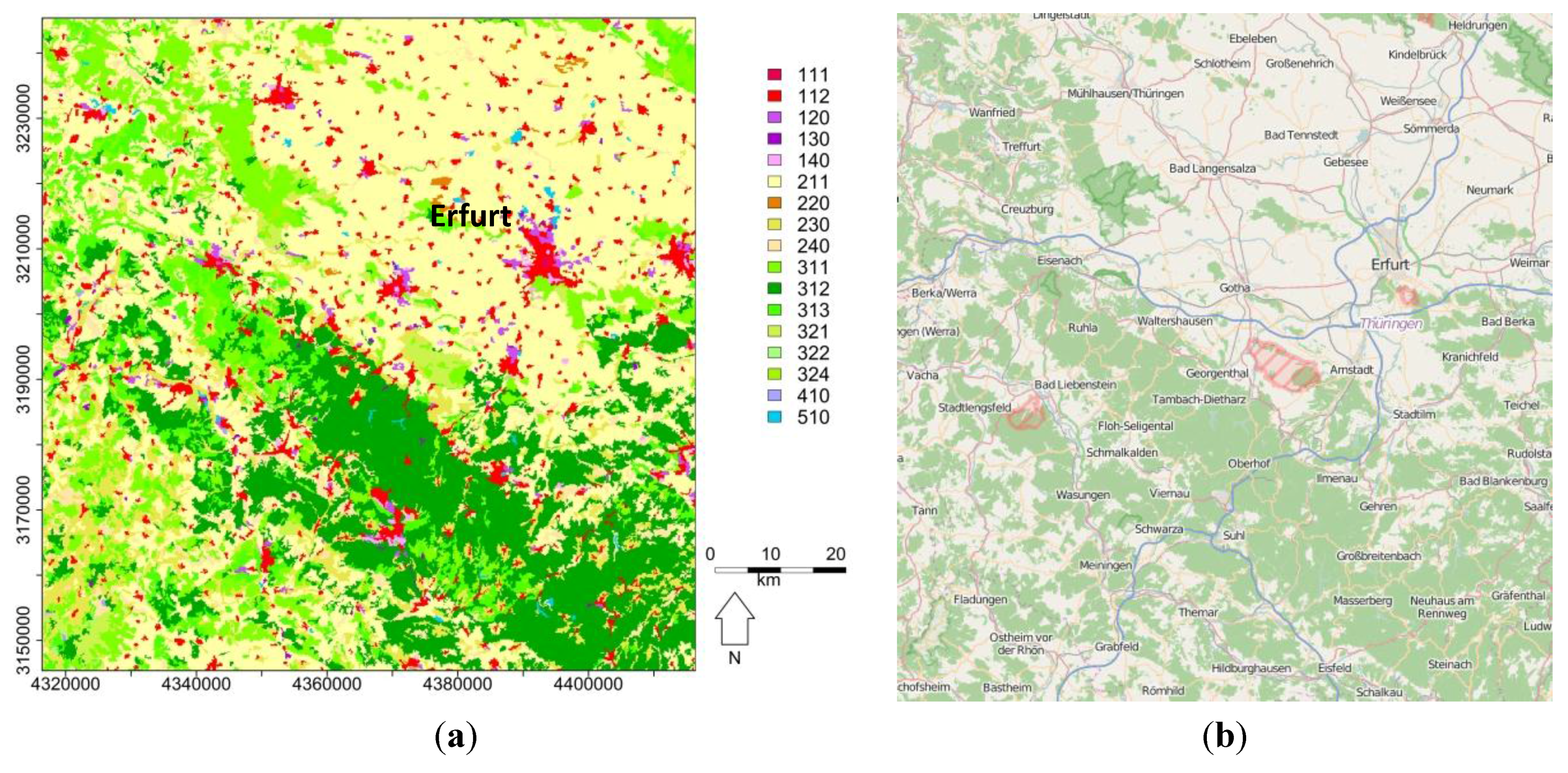
Figure 1.
Maps of the study area in Thuringia, Germany, showing the city of Erfurt. (
a) CORINE Land Cover Map 2006. See
Table 1 for class definitions. (
b) Street map © OpenStreetMap contributors.
Figure 1.
Maps of the study area in Thuringia, Germany, showing the city of Erfurt. (
a) CORINE Land Cover Map 2006. See
Table 1 for class definitions. (
b) Street map © OpenStreetMap contributors.
Table 2 shows the number of training pixels for each CORINE class, it follows the distribution of dominant classes of the overall CORINE map. The number of training pixels per class was capped at a maximum of 20,000 but some classes had fewer pixels in the polygon eroded CORINE image band. Bare rocks were masked out from the analysis due to their small sample size.
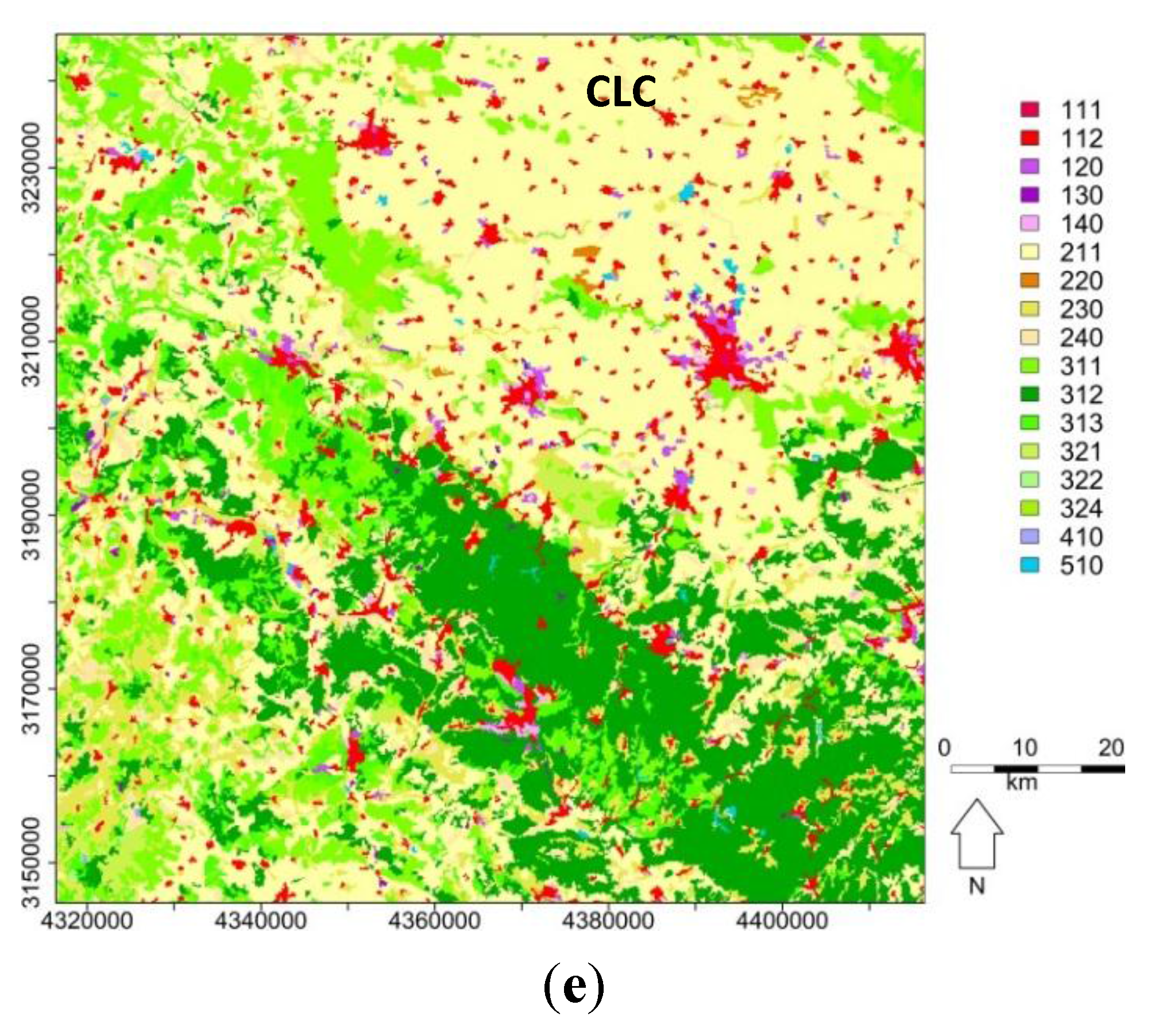
The hybrid CORINE land cover map for the study area and an OpenStreetMap quicklook are shown in
Figure 1. The study area is a homogeneous landscape covered by a large expanse of non-irrigated agricultural land (211), punctuated by permanent crops (220), mainly vineyards and fruit trees, pastures (230) consisting of small linear features on more marginal land often following landscape features such as rivers and the transport network, broadleaf (311), coniferous (312) and mixed forests (313) on the steeper and higher ground and discontinuous urban fabric (112) in the towns and villages.
The largest city appearing in red is Erfurt (
Figure 1). The elevation of the study region varies from 86 m to 973 m (mean = 388 m). After polygon erosion and training pixel selection, the signatures of the hybrid CORINE classes were calculated from the training pixels.
4. Discussion
The best of the classifiers is the RFTEXSRTM random forest, which uses the SAR backscatter images, HH texture band and SRTM bands as inputs. The out-of-bag error rate of the RFTEXSRTM classifier over the training sites is 31.6%, showing an accuracy of 68.4% and a κ = 0.63. Given the large number of land cover classes, this is a relatively low error rate considering that some of the non-matching pixels are likely due to the mapping scale differences and to real land cover change between 2006 and 2014.
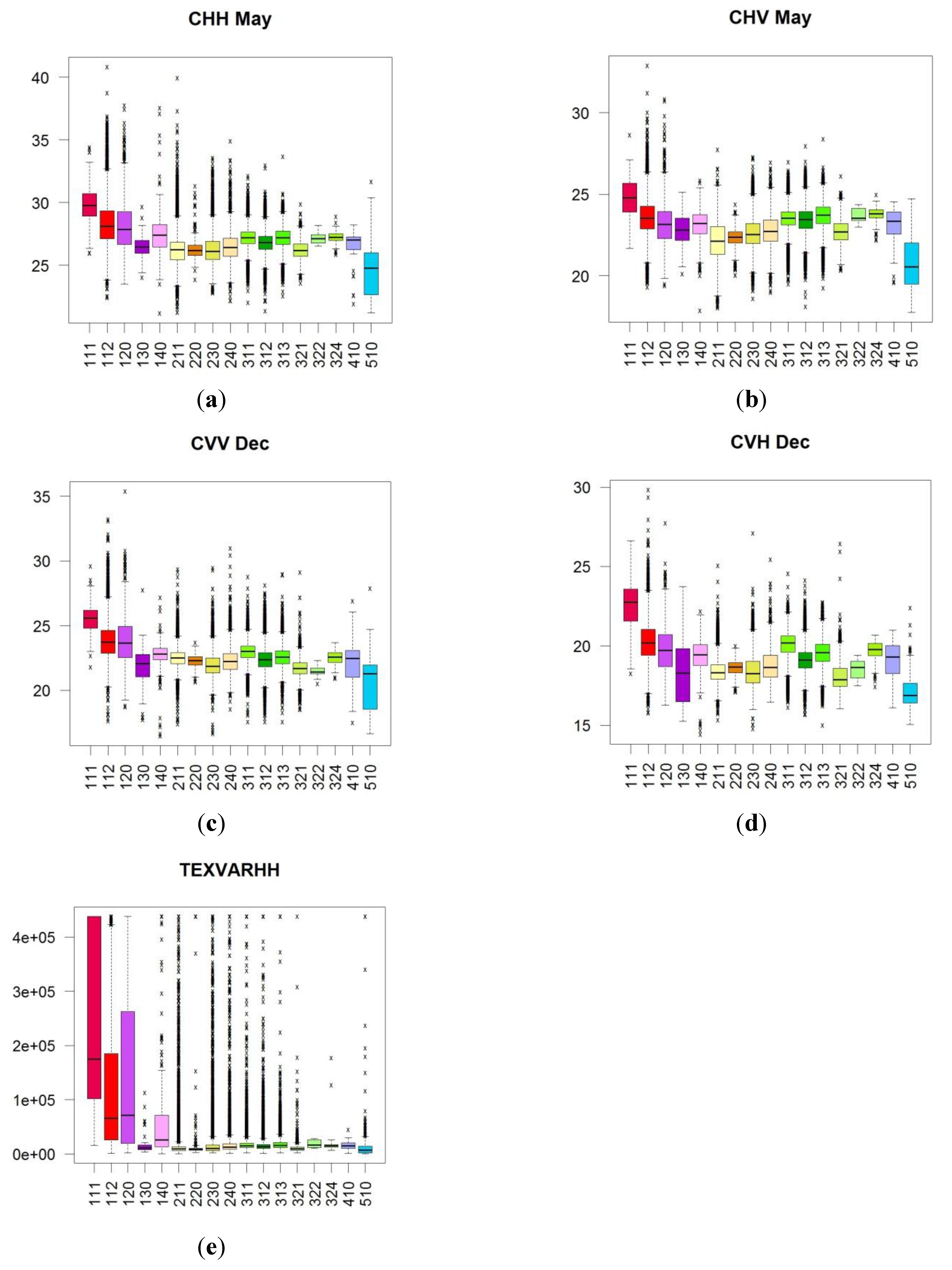
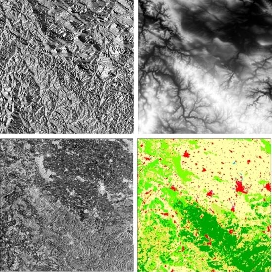
A visual comparison of the SAR texture band at HH polarisation in
Figure 4e with the CORINE land cover map in
Figure 1a shows that the texture is a good discriminator for urban land cover types while the backscatter intensities highlight vegetated areas very distinctively. Sentinel-1A is a C-band radar and hence the backscatter signal will originate from the top layer of any vegetation canopy. The use of a summer and winter acquisition enables a much better discrimination of agricultural cropland (seasonal vegetation cover) and forests (permanent vegetation cover), which would be confused by a single summer acquisition due to the similarities of volume scattering at C-band in forest and agricultural canopies. Single-date C-band radar backscatter intensity bands cannot distinguish very well between forested areas and dense agricultural crops, hence a radiometric classification of a single image is likely to lead to high rates of classification errors.
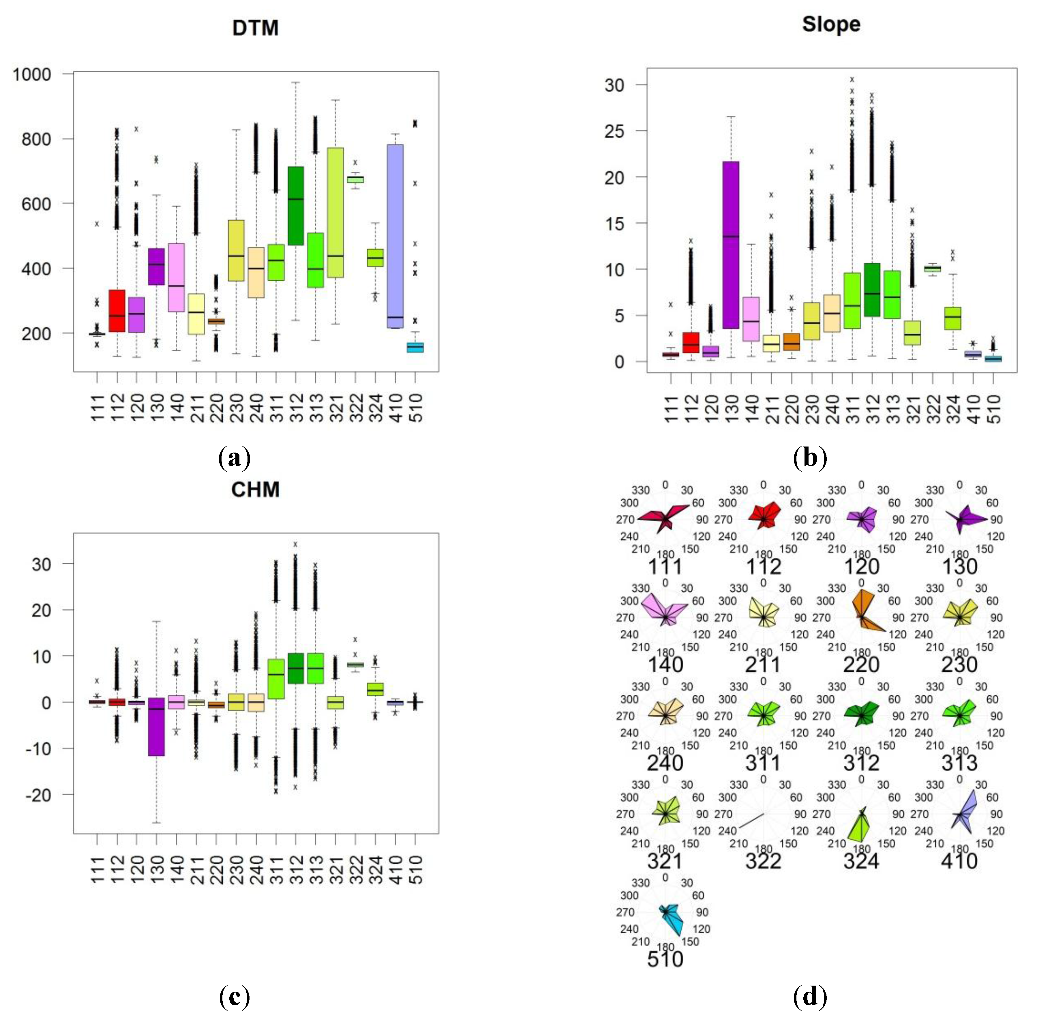
The slope map in
Figure 5b provides a more robust delineation of areas that are covered by forests than the single-date radiometry from SAR because of the structure of the landscapes in this region where steep slopes are often forested. The aspect of a hill side (
Figure 5c) can affect land use decisions, since south-facing slopes have higher insolation than north-facing ones.
Figure 6 shows that the Sentinel-1A imagery shows much more spatial detail than the original CORINE map because of the coarse minimum mapping unit of the CORINE land cover map of 25 ha. This characteristic difference in mapping scale makes a direct comparison of the two datasets difficult.
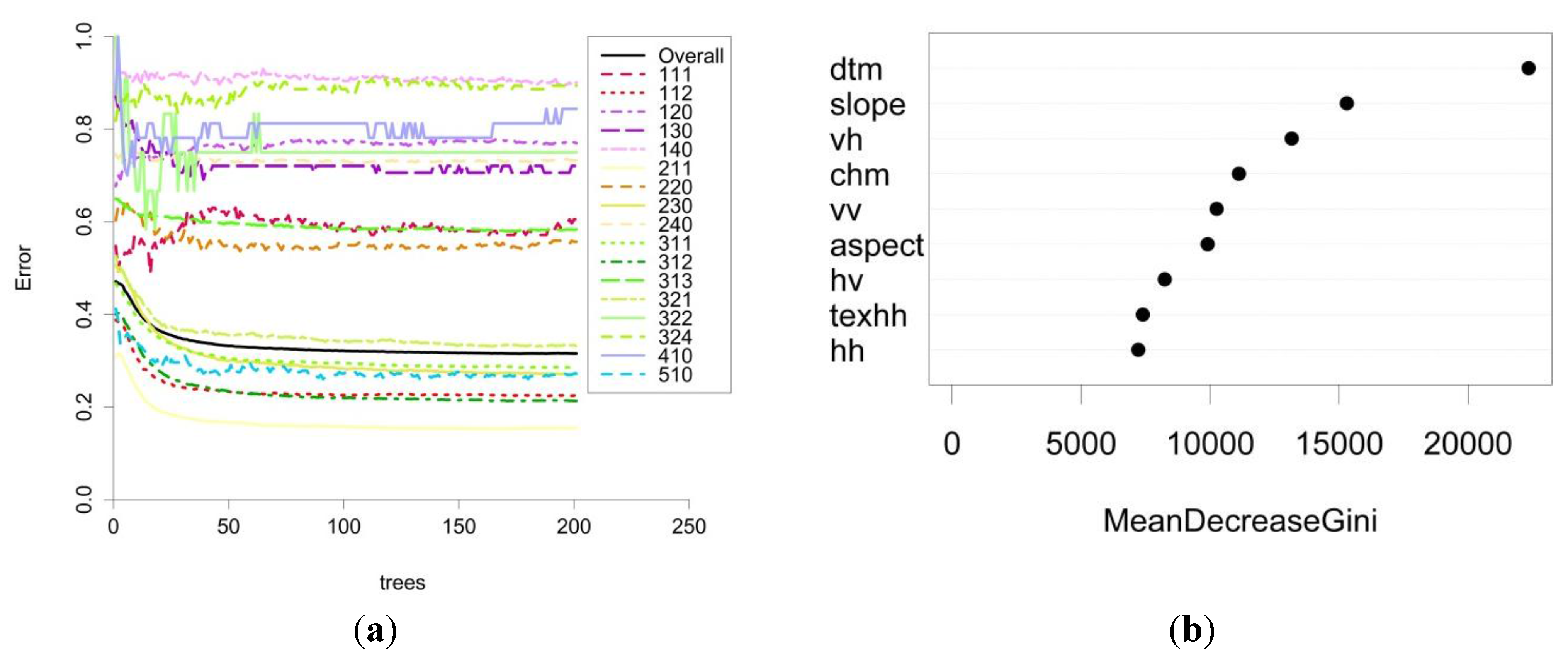
Using too few decision trees in a random forest can deteriorate the classification results. It is therefore important to check how many decision trees are required to achieve a stable error rate of the classification. Generally, the more trees are added, the more accurate the classification. In reality the error rate of the random forest decreases more slowly as more trees are added and approaches a limit when the number of trees is large enough. Here, 201 trees provided a number with stable error rates (
Figure 7a).
The findings of this study show that geomorphometric information on the landscape structure can improve classification accuracy when used in a random forest classification approach. While terrain shape alone cannot discriminate between CORINE land cover types, it can help the random forest classifier to distinguish between agricultural crops and forest cover classes that would otherwise appear very similar in a purely radiometric classification.
5. Conclusions
Several random forest classifications with different combinations of input bands are compared. Post-classification mode filtering was applied to improve the classified maps. The results show that the random forest with all Sentinel-1A SAR intensity bands from May and December, the HH texture band and four SRTM-derived terrain bands (DTM, CHM, SLOPE and ASPECT) gives the highest classification accuracy (68.4%) based on the out-of-bag error rates over the randomly selected CORINE 2006 training sites. The classification approach presented here uses the largest number of land cover classes derived from SAR imagery to date, compared to a thorough review of the literature. 27 classes were defined based on a hybrid level 2/3 CORINE nomenclature, of which 17 were found in the study area. In comparison to other types of landscapes in the CORINE mapped area, such as the heterogeneous landscapes of the UK, the study area is relatively simplistic and provides a good test site. The information content in the geomorphometric data layers is highly dependent on the landscape type studied. The applicability to more complex classes will need to be demonstrated in the future.
In its operational phase, Sentinel-1 Interferometric Wide-Swath Mode data will be the default acquisition mode over land areas. Sentinel-1 will thus provide interferometric digital surface models that could in principle allow the derivation of a DTM, CHM, slope and aspect maps to update the SRTM data. However, even with a 6 day temporal baseline, the temporal decorrelation will hinder the generation of DTMs using C-band. Only a passive Sentinel-1 chaser satellite to acquire bistatic interferometric data can alleviate the temporal decorrelation problem. The achievable accuracy of an elevation dataset from Sentinel-1 would be improved significantly if ESA launched a Sentinel-1 Convoy mission with a receive-only SAR sensor, operating in tandem with Sentinel-1A or 1B as a bistatic SAR.
In conclusion, this study shows that Sentinel-1 is an important data source that can complement land cover mapping, especially under cloudy conditions. Random forests and other machine learning approaches achieve high classification accuracy when used in conjunction with geomorphometric data from a DTM and CHM and prior information on past land cover.
Under such circumstances, an operational SAR-based land cover monitoring service for a rapid mapping of CORINE land cover change is conceivable if the transferability of the method can be demonstrated. Furthermore, the hyper-temporal coverage of Sentinel-1A (and 1B) will allow the computation of multi-temporal metrics. These metrics have the potential to further improve the delineation of CORINE relevant classes as demonstrated in previous studies [
12,
16]. This will provide the focus of future research.


