Article

Self-Guided Segmentation and Classification of Multi-Temporal Landsat 8 Images for Crop Type Mapping in Southeastern Brazil

by
Bruno Schultz
1,2,*,†,
Markus Immitzer
2,†,
Antonio Roberto Formaggio
1,
Ieda Del’ Arco Sanches
1,
Alfredo José Barreto Luiz
3 and
Clement Atzberger
2
1
Divisão de Sensoriamento Remoto (DSR), Instituto Nacional de Pesquisas Espaciais (INPE), Avenida dos Astronautas 1758, São José dos Campos, 12227-010 SP, Brazil
2
Institute of Surveying, Remote Sensing and Land Information (IVFL), University of Natural Resources and Life Sciences, Vienna (BOKU), Peter Jordan Strasse 82, 1190 Vienna, Austria
3
Embrapa Meio Ambiente, Caixa Postal 69, Jaguariúna, 13820-000 SP, Brazil
*
Author to whom correspondence should be addressed.
These authors contributed equally to this work.
Remote Sens. 2015, 7(11), 14482-14508; https://doi.org/10.3390/rs71114482
Submission received: 3 September 2015 / Revised: 16 October 2015 / Accepted: 26 October 2015 / Published: 30 October 2015

Abstract

:
Only well-chosen segmentation parameters ensure optimum results of object-based image analysis (OBIA). Manually defining suitable parameter sets can be a time-consuming approach, not necessarily leading to optimum results; the subjectivity of the manual approach is also obvious. For this reason, in supervised segmentation as proposed by Stefanski et al. (2013) one integrates the segmentation and classification tasks. The segmentation is optimized directly with respect to the subsequent classification. In this contribution, we build on this work and developed a fully autonomous workflow for supervised object-based classification, combining image segmentation and random forest (RF) classification. Starting from a fixed set of randomly selected and manually interpreted training samples, suitable segmentation parameters are automatically identified. A sub-tropical study site located in São Paulo State (Brazil) was used to evaluate the proposed approach. Two multi-temporal Landsat 8 image mosaics were used as input (from August 2013 and January 2014) together with training samples from field visits and VHR (RapidEye) photo-interpretation. Using four test sites of 15 × 15 km2 with manually interpreted crops as independent validation samples, we demonstrate that the approach leads to robust classification results. On these samples (pixel wise, n ≈ 1 million) an overall accuracy (OA) of 80% could be reached while classifying five classes: sugarcane, soybean, cassava, peanut and others. We found that the overall accuracy obtained from the four test sites was only marginally lower compared to the out-of-bag OA obtained from the training samples. Amongst the five classes, sugarcane and soybean were classified best, while cassava and peanut were often misclassified due to similarity in the spatio-temporal feature space and high within-class variabilities. Interestingly, misclassified pixels were in most cases correctly identified through the RF classification margin, which is produced as a by-product to the classification map.

Graphical Abstract

1. Introduction

Monitoring projects yielding agricultural information in near-real-time and covering a large number of crops are important [1,2]. This is particularly true for Brazil, which is one of the largest countries of the world and a main producer and exporter of agricultural commodities [3]. For this reason, in Brazil, the use of remote sensing (RS) data for automated crop classification has been largely explored. Most studies used either moderate spatial resolution data from Moderate Resolution Imaging Spectroradiometer (MODIS) Aqua and Terra satellites [4,5], or images from Landsat and Landsat-like satellites [6,7,8,9]. Field size and crop type are the most important determinants for the sensor selection. Operationally until 2013, in Brazil only sugarcane in Middle-South was remotely monitored (e.g., Canasat Project) [10].
For crop identification, MODIS offers the advantage of a daily revisit frequency. This increases the possibility of obtaining cloud free data [11,12] and makes it possible to track crops along the season. The derived temporal profiles of vegetation indices such as Normalized Difference Vegetation Index (NDVI) can be used for automatic classification and land cover mapping [5,13,14]. The multi-temporal data is also very useful for estimating crop production and yield [15]. However, smaller fields cannot be mapped with this data [16,17,18] as the spatial resolution is too coarse (e.g., 250 m). Luiz and Epiphanio [19] for example, have shown that fields smaller than 10 ha have a high percentage (≥1/3) of mixed pixels at the crop boundaries. Rudorff et al. [18] and Yi et al. [18] have demonstrated that the 6.25 ha MODIS pixel size is not useful to map smallholdings in Rio Grande do Sul State. Lamparelli et al. [16] demonstrated that soybean fields in Paraná State should be at least 30 ha for being efficiently mapped. Unmixing approaches [20,21,22] and blending algorithms [23,24,25,26] are not yet accurate enough to counterbalance the relatively coarse spatial resolution of MODIS and other medium/coarse resolution sensors.
Compared to MODIS, Landsat offers a much better spatial resolution (≈30 m). This contributes positively to crop classification. Cowen et al. [27], for example, stated that the required spatial resolution of remotely sensed data needs to be at least one half the size of the smallest object to be identified in the image. Even in Brazil, fields are sometimes only a few hectare large demonstrating the need for deca-metric sensors like Landsat, ASTER, Sentinel-2, Resourcesat-2 and CBERS-3. The disadvantage of Landsat relates to its low revisit frequency of 16 days (eight days if Landsat-7 and 8 are combined) [28]. Together with cloudiness, this may drastically reduce the number of high quality observations [29].
When pixel sizes are relatively small compared to object sizes, traditional pixel-based classification approaches may not be the best choice for land cover mapping. With such data sets, object-based classification approaches have several advantages compared to pixel-based approaches [30,31,32,33,34]. For example, using object-based image analysis (OBIA), the impact of noise is minimized. At the same time, textural features may be integrated for improving classification results [9,35]. Also, shape and context information can be used for the classification [30,32]. The listed features are not readily available within pixel-based approaches. Consequently, object-based approaches have been widely used for crop classification in Landsat-like images [9,33,36,37,38,39,40,41,42].
Regarding suitable segmentation algorithms, a variety of alternatives exist [43]. All algorithms have advantages and disadvantages, and there is no perfect segmentation algorithm for defining object boundaries [44,45,46]. Many scientific studies rely on the Multiresolution Segmentation algorithm [9,30,34,37,40,41,42,47,48,49,50]. This algorithm starts with one-pixel image segments, and merges neighboring segments together until a heterogeneity threshold is reached [51]. Widely used alternatives include the MeanShift algorithm [52,53] or approaches based on watershed-segmentation [54]. A recent overview of trends in image segmentation is provided in Vantaram and Saber [55].
Using OBIA, the main problem relates to the fine-tuning of segmentation parameters [9,31,41]. Only well-chosen segmentation parameters ensure good segmentation results. Manually defining suitable parameter sets can be a time-consuming approach, not necessarily leading to optimum results [34,48,49]. Obviously, the manual approach is also highly subjective and therefore not always reproducible. A visually appealing segmentation also does not necessarily lead to a good classification [56]. For this reason, in supervised segmentation one integrates the segmentation and classification tasks.
In the implementation of supervised segmentation by Peña et al. [42] a range of segmentation parameters are applied to the multi-spectral imagery followed by an assessment of the geometrical accuracy of the resulting segments. The geometric quality of the segmentation outputs is estimated by applying the empirical discrepancy method, which consists of a comparison of the derived segment boundaries with an already computed ground-truth reference. An alternative approach was recently presented by Stefanski et al. [57]. In their supervised segmentation approach, the most suitable segmentation parameters are identified by running, for each segmentation, a supervised classification and keeping the parameter set minimizing the classification errors (out-of-bag).
In this contribution, we further develop the approach by Stefanski et al. [57] and present a fully automated, supervised segmentation and classification approach combining multiresolution segmentation and Random Forest (RF) classification. The fully autonomous workflow for supervised object-based classification also includes a robust feature selection procedure. Suitable segmentation and classification parameters are automatically identified starting from a fixed set of randomly selected and manually interpreted training samples. Using a large data set of independent validation samples, we demonstrate that the approach leads to a near optimum classification results when mapping five (crop) classes within an agricultural area located in South-East Brazil, using multi-temporal spectral information from the Landsat 8 sensor as input.

2. Material

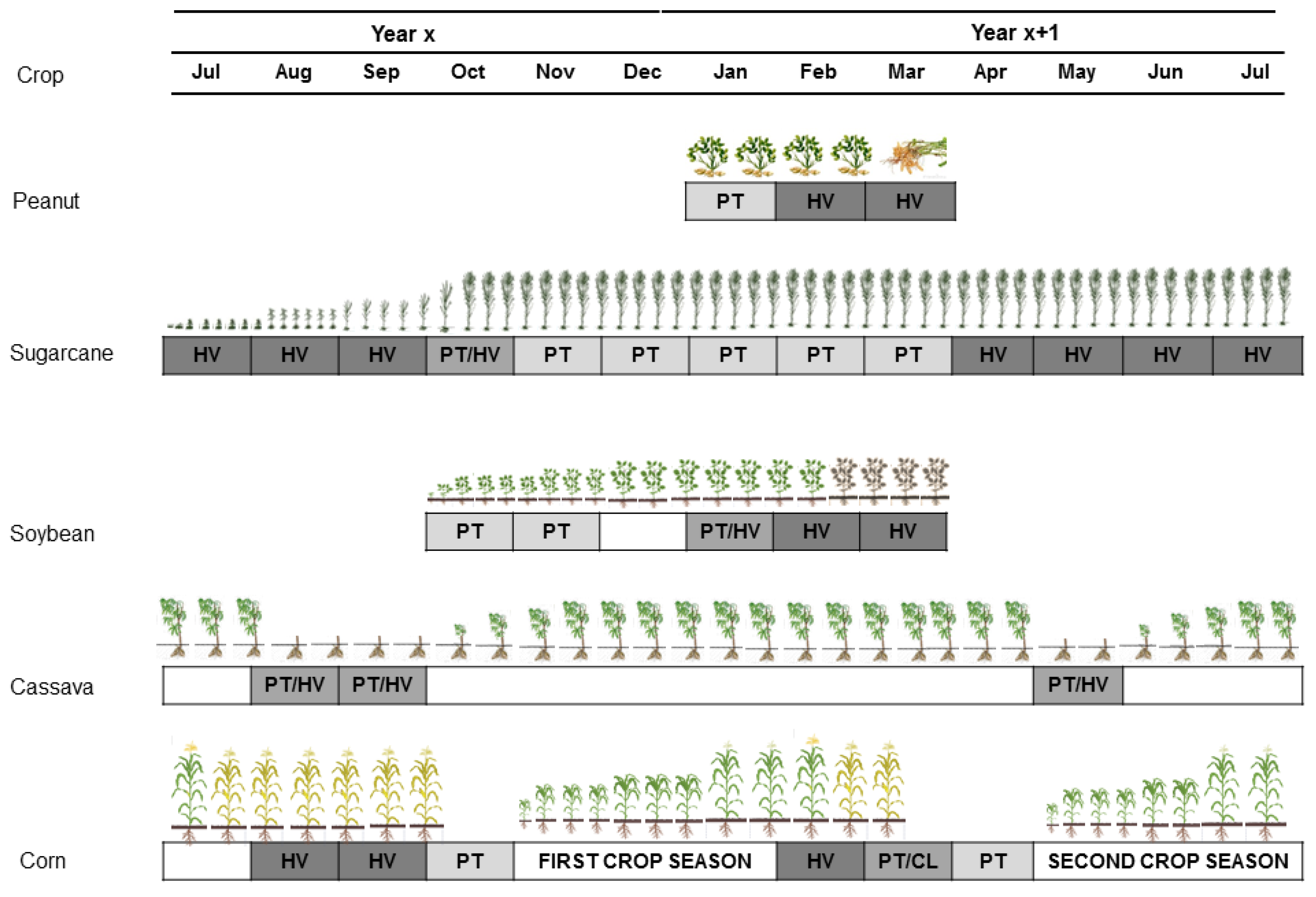
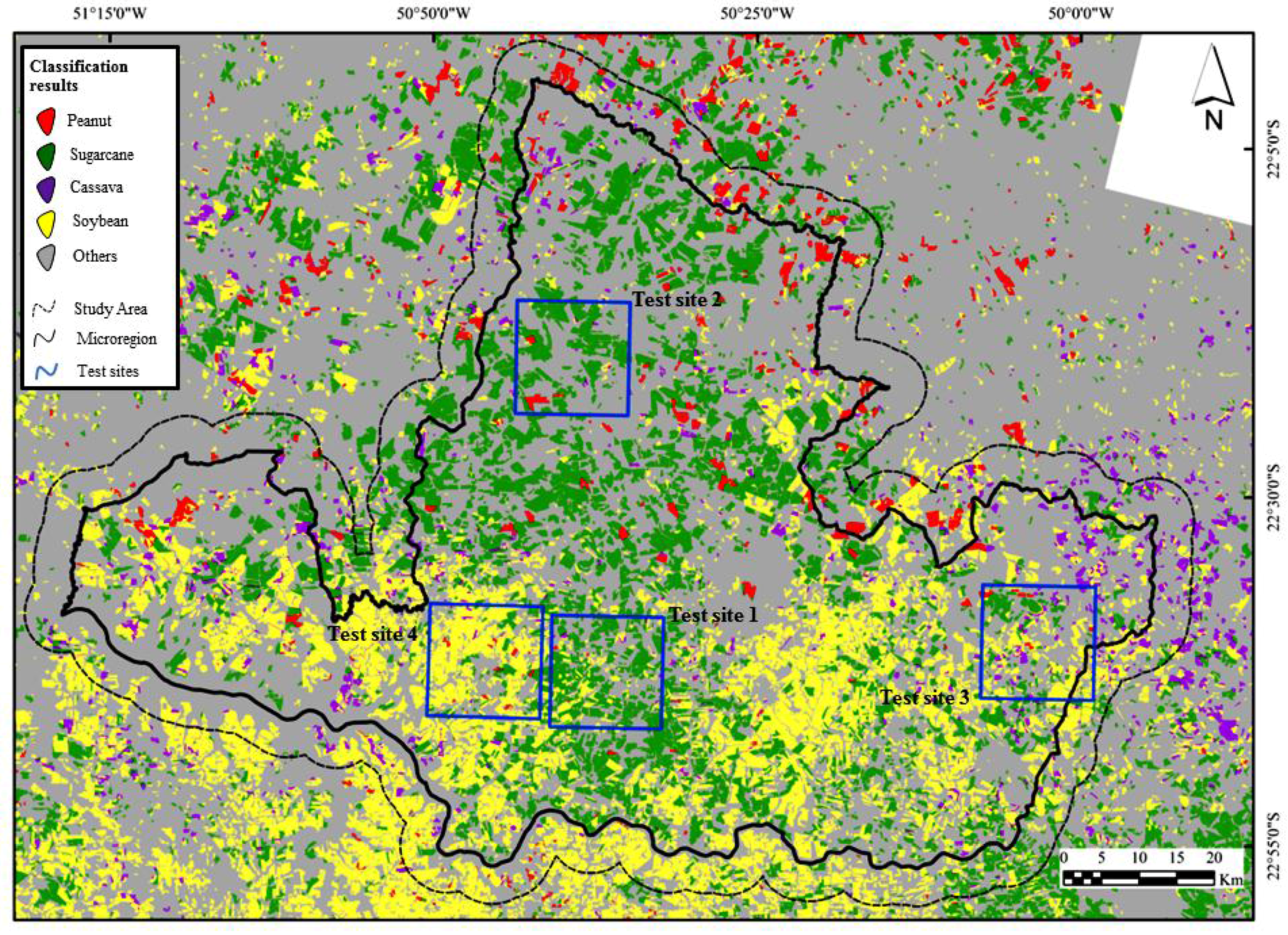
2.1. Study Site and Crop Calendar

The selected study site is located in the Assis microregion in South-East Brazil (south of São Paulo State), one of the major agricultural production areas of the country (mainly sugarcane and a number of summer crops). In Brazil, a microregion is a legally defined administrative unit consisting of groups of municipalities bordering urban areas used by IBGE (Brazilian Institute of Geography and Statistics) [58].
The study region occupies an area of roughly 715.000 ha. The climate in the region is sub-tropical with average annual temperatures of 21.3°C and annual precipitation of 850 mm [59]. Four main soil types are found in the region (Figure 1a). The study site is fully covered by Landsat paths 220 and 221 (rows 75 and 76) (Figure 1b). Terrain is hilly with elevations ranging from 275 to 645 m above sea level (a.s.l.) (Figure 1b). Several other studies were conducted in São Paulo State [6,9,20] but not yet in the Assis microregion.
Figure 1. Soil types (A) and digital elevation model (DEM) (B) of the study area. Soil names are shown according to Word Reference Base (WRB–FAO) and São Paulo Environmental System (2015), respectively. DEM from Advanced Spaceborne Thermal Emission and Reflection Radiometer (ASTER) in 90 m resolution. In (B) are also shown the two Landsat paths covering the study area.
Remotesensing 07 14482 g001
The Assis microregion was selected as a test site because it is typical for Brazilian agricultural production areas with large sugarcane plantations, but also many other (summer) crops, occupying together roughly ¾ of the land. According to the official agricultural production data (from IBGE in 2013 at municipal level), the Assis’ main crops are sugarcane (32%), soybean (20%), corn (20%), cassava (2%) and peanut (1%). The area has thus a very high proportion of agricultural land use. Within the São Paulo State, the region is the largest producer of corn and soybean [58]
The typical crop calendar (double cropping) for the Assis microregion is shown in Figure 2. The average crop cycle length is 100–120 days with multiple sowing and harvesting periods. Thus, the same crops may appear at different times during the year.
Figure 2. Crop calendar of the main crops of the Assis microregion: peanut, sugarcane, cassava, corn and soybean. PT (light grey): planting; HV (dark grey): harvesting; CL (light grey): clearing. In white: crops keep green during the period. Note that field work was done in the first half of March.
Remotesensing 07 14482 g002
Sugarcane and cassava crops are semi-perennial crops and have a much longer vegetative period compared to the other crops of the area. Sugarcane can keep green between 1 and 1.5 years before being harvested. Sugarcane fields are mostly reformed at the beginning of the year using forage plants such as soybean and peanut [10]. The harvest can start at the beginning of April and last until December [60]. Most sugarcane fields are harvested during the month of October [61]. Cassava is planted either in August/September or in May. It can be managed in two different forms: one or two years. For the two-year cassava, the plants are trimmed after one year and then are kept one more year on the field.
Corn is cropped in the Assis microregion mainly as secondary crop (called “Safrinha”). In 2013, almost 74% of the corn areas were planted in March and April after soybean harvest [62]. No information about corn could be collected at the field work because the safrinha season started only in the end of April/beginning of May (Figure 2). Hence, in this study, corn is part of the class others.
Typical appearances of sugarcane, soybean, cassava and peanut fields from Assis microregion are shown in Figure 3 at different times of the year using RapidEye and Landsat 8 imagery. Note that cassava and peanut fields have a similar spectral behavior as soybean (in bands B4, B5 and B6). Photos taken during the field campaign are also shown.
Figure 3. Example images for the classes peanut, cassava, sugarcane, soybean and others (field boundaries in white). Note that the class “others” includes not only agricultural areas but also constructions, water, etc. The photos from the field work were made around 40 days after the “Mid Season” images were taken (e.g., in March). The RapidEye image is shown in band combination 453 and was taken July 2011. The Landsat 8 images are shown in band combination 564 and were taken in August 2013 (Late Season) and January 2014 (Mid Season).
Remotesensing 07 14482 g003

2.2. Satellite Imagery

For this study, Landsat 8 and very high resolution (VHR) RapidEye images were used. Landsat 8 (Operational Land Imager, OLI) records nine spectral bands with a ground sampling distance (GSD) of 30 m [63] (Table 1). RapidEye records the spectral reflectance in five spectral bands at a GSD of 6.5 m [50]:
  • Two multi-spectral Landsat 8 image mosaics were used for image segmentation and classification. Seven additional mosaics from Landsat 7 (Enhanced Thematic Mapper Plus, ETM+) and Landsat 8 (OLI) images were used for the generation of reference information.
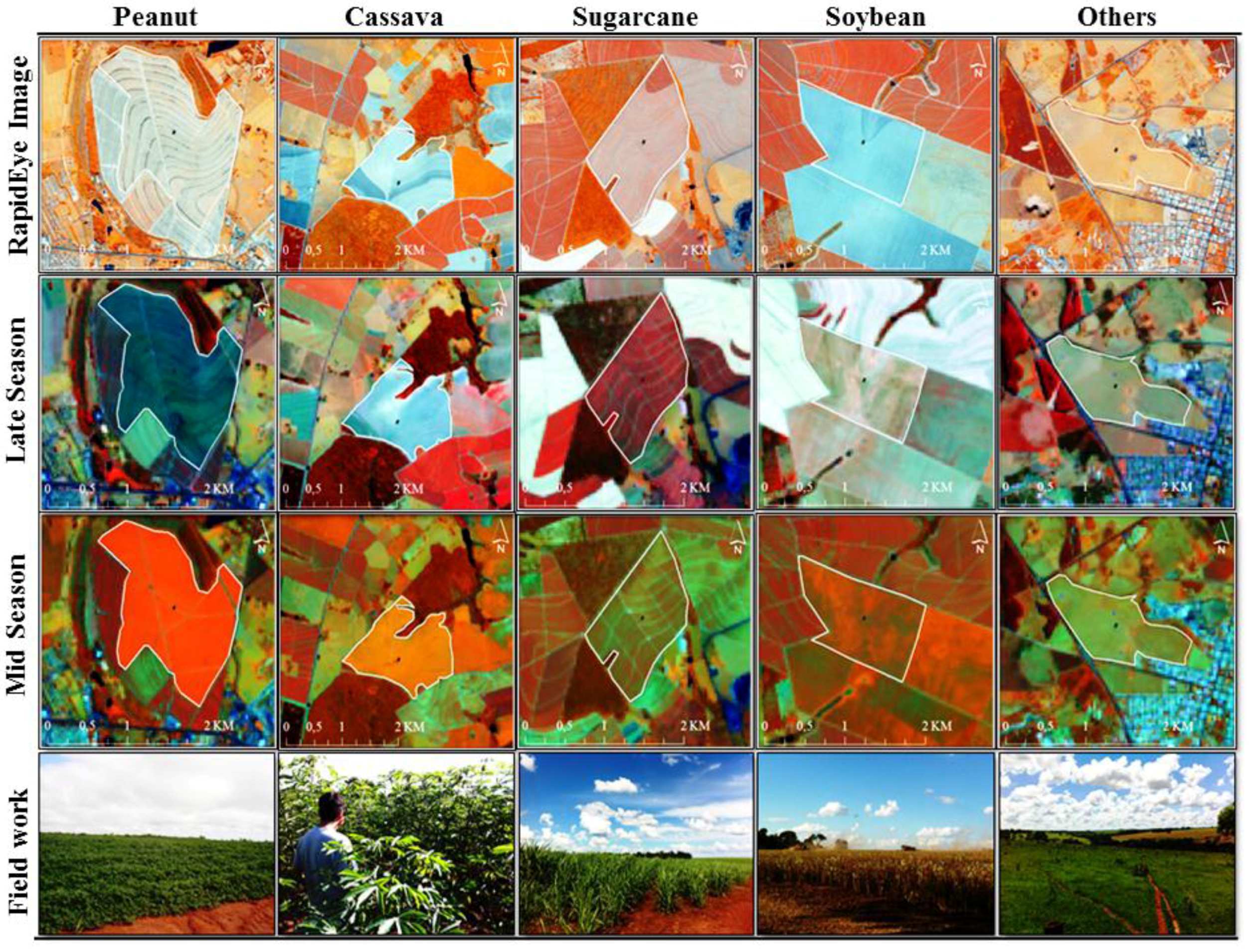
  • One RapidEye mosaic from four images was used as ancillary data for assisting in the visual photo-interpretation and for (manual) field delineation as suggested by Forster et al. [44].
Landsat 8 Imagery. To cover the study area, three Landsat 8 (OLI) scenes from paths 221 and 222 are necessary (paths/rows 222/75, 222/76 and 221/76) (Figure 1b). The two paths result in a nine-day difference of images from adjacent paths. All images were level-one terrain-corrected (L1T) products (USGS, 2014) and derived from USGS web-site (http://earthexplorer.usgs.gov). All images had less than 25% cloud cover.
Table 1. Basic characteristics of Landsat 8 and 7 Operational Land Imager (OLI) and Enhanced Thematic Mapper Plus (ETM+) and RapidEye.
Images DescriptionLandsat 8Landsat 7RapidEye
Sensor nameOperator Land Imager (OLI)Enhanced Thematic Mapper (ETM+)Multispectral Imager (MSI)
Satellite (number)115
Equator Time (hour)±11:00±10:10±10:30
Radiometric resolution (Bits)16812
Ground Sampling Distance (m)30306.5
Spectral bands (nm)
Aerosols430–450----
Blue450–520450–520440–510
Green530–590530–610520–590
Red640–670630–690630–685
Red-Edge----690–730
NIR850–880780–900760–850
SWIR1570–16101550–1750--
2110–22902090–2350--
Panchromatic (PAN)500–680520–900--
Cirrus1360–1380----
For the image segmentation and classification, two Landsat mosaics were created using three Landsat 8 images for each (Table 2):
  • A late-season mosaic combining scenes from 21 August 2013 and 30 August 2013,
  • A mid-season mosaic using scenes from 28 January 2014 and 6 February 2014.
The chosen images had the highest quality from all images of the 2013/2014 growing season. All other images had high cloud coverage.
To create the Landsat 8 mosaics, the two images from Path 222 (222/75 and 222/76) were directly combined (same day imagery). This combined image is hereafter referred to as the “parent” image. The third image (221/76), hereafter named as the “son” image, was acquired nine days later. Using the overlapping parts of parent and the son images, a linear transfer function was derived for each spectral band to radiometrically match the son image to the parent image [40,64].
For the creation of reference samples (see next section), seven other Landsat (OLI/ETM+) mosaics were created in a similar way using the images listed in Table 2:
  • Three mosaics between the late-season and mid-season (from October, November and December), and
  • Four mosaics after mid-season (from February, March, April and May)
VHR Rapid Eye Imagery. RapidEye images were used as ancillary data to manually delineate the crop areas (top row of Figure 3). This data was not used for classification or segmentation. Images from paths 285–288 and rows 15–19 were used (Table 2). Two different dates were necessary to cover the Assis microregion (3 July 2012 and 27 November 2012). The 2012 image collection was acquired from the National Institute for Space Research (INPE) catalog [65].
Table 2. Images (Landsat and RapidEye) used for the study.
Image IdentifierLandsat 8 and 7 (Path/Row)RapidEye (Path/Row)
222/75222/76221/76285/15286/15287/15288/15
16/17/1816/17/1816/17/1816/17/18
Images for manual field delineation21 Aug. 201321 Aug. 201330 Aug. 201303 Jul. 201203 Jul. 201203 Jul. 201227 Jul. 2012
28 Jan. 201428 Jan. 201406 Feb. 2014
Images for visual photo-interpretation21 Aug. 201321.Aug.1330 Aug. 2013--------
08 Oct. 201308 Oct. 201309 Oct. 2013--------
09 Nov. 201309 Nov. 201302 Nov. 2013--------
11 Dec. 201311 Dec. 201304 Dec. 2013--------
28 Jan. 201428 Jan. 201406 Feb. 2014--------
13 Feb. 201313 Feb. 201314 Feb. 2014--------
01 Mar. 201301 Mar. 201310 Mar. 2013--------
02 Apr. 201302 Apr 201311 Apr. 2013--------
04 May 201304 May. 201313 May 2013--------
Images for segmentation and classification21 Aug. 201321 Aug. 201330 Aug. 2013--------
28 Jan. 201428 Jan. 201406 Feb. 2014--------
Total number of consulted images9991111

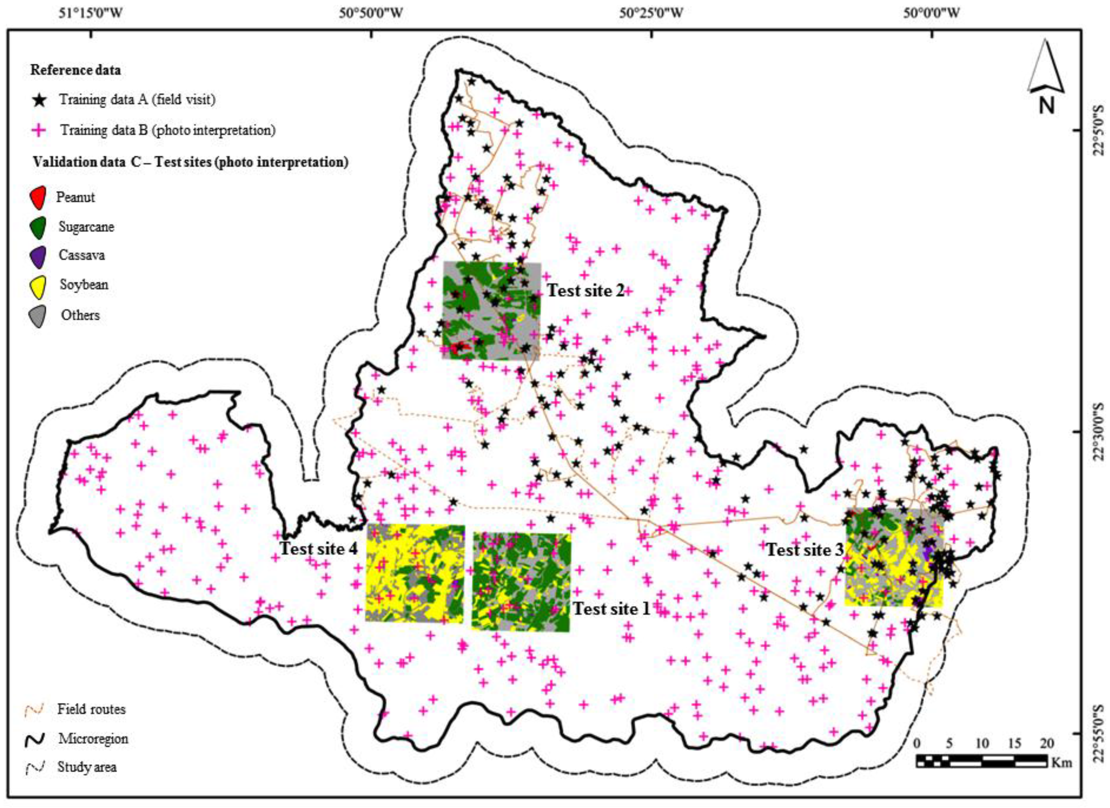
2.3. Reference Data Collection

A large set of reference samples (points and segments) were created for model training and validation (Figure 4 and Table 3):
(A)
Reference samples from field visit (n=177),
(B)
Reference samples obtained through manual photo interpretation (n=500), and
(C)
Manually delineated and interpreted fields (n=2502).
Samples (A) and (B) were pooled and used for model training. The calibrated model was validated using samples (C).
Table 3. Summary of available reference samples for training (A and B) and validation (C) (visually interpreted).
Reference dataData typeInterpretationPeanutSoybeanCassavaSugarcaneOthersTotal
Training samples (A)PointsField visit2433373251177
Training samples (B)PointsPhoto interpretation11921796284500
Validation samples—test sites (C)PolygonsPhoto interpretation96893349512752502
Point samples. During a field campaign (7–12 March 2014), 177 sample locations were identified by GPS, visited and assigned to one of the five classes (samples A—black stars in Figure 4): peanut (24), sugarcane (30), cassava (38), soybean (35) and others (57). Amongst those 177 samples, 91 were pre-defined based on random sampling. The remaining 86 samples were added ad hoc during the field work as three crops (cassava, soybean and peanut) revealed only small spectral differences in the mid-season image. A GPS was used to navigate from one random point to the next.
To limit the travel distance, the field study had to be limited to four municipalities of Assis microregion (Figure 4): Campos, Novos Paulista, Quatá and Paraguaçú Paulista. As the field visit took place almost 1.5 months after the Mid-season image acquisition, care was taken to assign the class label corresponding to the date of image acquisition. Straw and germinating plants resulting from the cropping/harvest process were useful in this respect—as well as detailed agronomical knowledge of the crops and the study region [10,66]. Table 3 summarizes information about the field sampling points.
Figure 4. Reference information collected within the Assis microregion. Reference samples obtained through field visit are shown as black stars. Additional reference samples were obtained through photo-interpretation and are shown as magenta crosses. Four smaller test sites (named TS1 to TS4) were placed within the study area and field boundaries were manually delineated. The resulting segments were visually interpreted to yield reference polygons.
Remotesensing 07 14482 g004
After field work, additional 500 sample points (samples B) were randomly distributed over the Assis microregion and visually interpreted by experienced photo-interpreters using Landsat 8 imagery (Figure 4—red crosses), levering experienced gained during the field. Afterwards, samples (A) and (B) were merged together. We hereafter referred to them as “reference points”. In Figure 4, the two sample sets (A and B) can still be distinguished by their respective symbols.
Test Sites Photo-Interpretation. To permit assessment of segmentation quality and for creating additional reference samples for independent validation, four 15 km × 15 km test sites were placed over the study area (Figure 4). In these four test sites, field boundaries were digitized manually and the resulting segments were visually assigned to one of the five classes (samples C—Table 3). The field boundaries were delineated on the computer screen using RapidEye imagery and Landsat images acquired during mid- and late-season. The fields were digitized and interpreted by experienced photo-interpreters at INPE using a pre-defined visual classification protocol created using false color compositions: (OLI 564) and (ETM+ 453).
The four test sites occupy a total area of 900 km2. A summary of the collected reference polygons (n=2502) is given in Table 4. We will refer to samples (C) as “reference fields”. Note that the reference fields do not enter in the calibration stage (i.e., model development and training) but are solely used for independent model validation. Validation was done at pixel level yielding about 1 million pixels (900 km²) for the 2502 fields.
The first (TS1) and forth test site (TS4) had the largest number of sugarcane and soybean polygons, respectively. These are the two most important crops in the area. The second site (TS2) is important because the parcels in this test site show the highest variability in size and this across the five individual (crop) classes. The particularity of test site TS3 is the high number of cassava and peanut fields, which are almost absent in the other three test sites. Table 4 and Figure 4 also reveal that the spatial distribution amongst the four test sites is very different.
Table 4. Descriptive summary of reference information collected within four test sites (TS1 to TS4). Numbers to which we refer in the text are highlighted. The reported statistics relate to individual polygons. Polygons were manually digitized and visually interpreted. All areas are in ha.
Test SiteMetricsCrops (area in ha)OthersAverage & (total)
PeanutSoybeanCassavaSugarcane
TS 1Average4.6726.308.0140.8029.2833.39
Stand. Dev.--24.283.5550.8140.1228.58
Nº Parcels11267288252(n = 674)
TS 2Average76.0017.6623.95108.6045.0154.24
Stand. Dev.46.4816.01--108.7768.3459.03
N° Parcels613181289(n = 390)
TS 3Average62.9430.8621.8153.7626.0729.64
Stand. Dev.59.7838.7422.6570.4042.6344.66
N° Parcels22191760461(n = 759)
TS 4Average--38.8617.5144.7923.8033.14
Stand. Dev.--37.3513.5546.6732.7837.30
N° Parcels0331867273(n = 679)
allAverage65.1733.6217.9153.9830.5135.97
Stand. Dev.48.4135.8718.1669.9348.1851.03
N° Parcels9689334961275(n = 2502)

3. Methods

A general flowchart of the methodology applied in this work is shown in Figure 5. The various sub-tasks will be outlined in appropriate sub-sections.
Figure 5. Flowchart of the methodology applied in this work.
Remotesensing 07 14482 g005

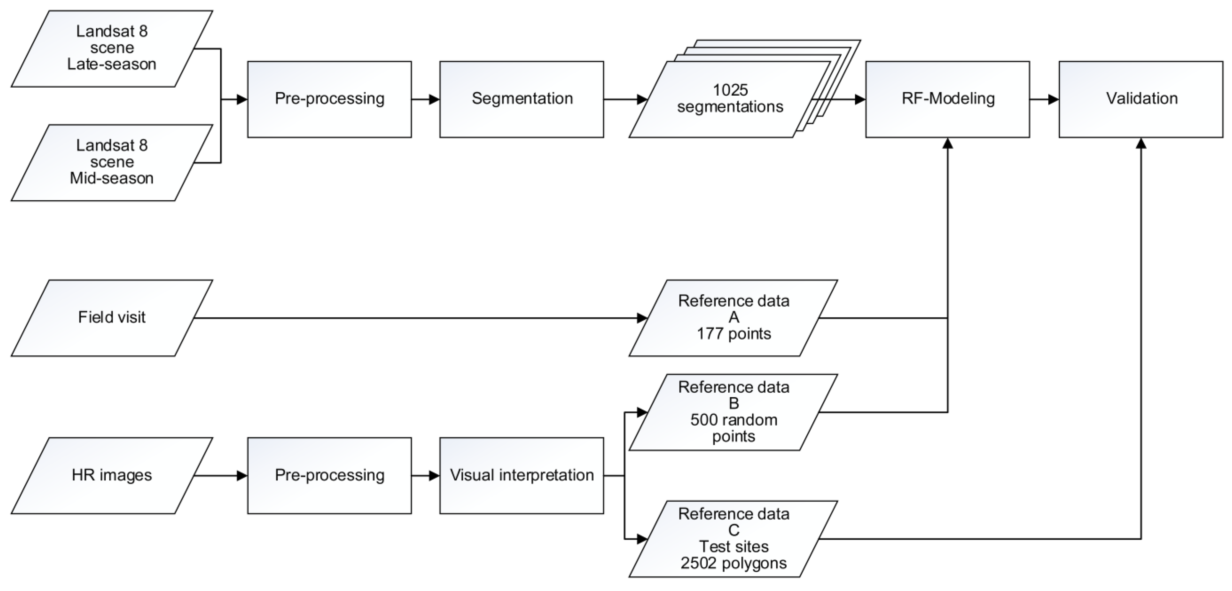
3.1. Image Segmentation and Data Extraction

We used the multiresolution segmentation (MRS) implemented in eCognition Developer 8 software for image segmentation. The software is extensively applied in OBIA studies [30]. MRS is a sequential region merging method starting with single pixels. It groups mutually similar adjacent pixel pairs to form initial segments. These segments are then iteratively merged with neighboring segments as long as the change in heterogeneity is below a user-defined threshold.
We used the two Landsat images as input data by stacking Red, NIR and SWIR 1 bands of the two images. The three bands were selected following several studies [9,10,66]. These three bands also show low inter-band correlation.
Instead of manually fine-tuning the software parameters, a wide range of different MRS were performed by altering parameter levels. We varied the scale value from 50 to 250 (step size 5), the shape and also the compactness weight from 0.1 to 0.9 (step size 0.2). The parameter combinations led to 1025 different segmentations which were exported in shape file format as well as GeoTIFFs.
Afterwards, for each segment and each segmentation, different attributes were calculated and exported in table format. Due to the similar spectral behavior of some classes also texture and shape information were used, which is also recommended by other studies (e.g., [9]):
(1)
The mean value and standard deviation of each spectral band for each of the two dates (6 × 2 × 2 = 24 variables);
(2)
Maximum difference and brightness (2 variables);
(3)
The normalized difference vegetation index (NDVI) for each date (2 variables);
(4)
The maximum, medium and minimum mode of the segments in each spectral band for each date (3 × 6 × 2 =36 variables);
(5)
The quartiles to the segments in each spectral band and each date (5 × 6 × 2 = 60 variables);
(6)
The GLCM (Gray-Level Co-Occurrence Matrix) homogeneity, GLCM contrast, GLCM dissimilarity, GLCM entropy, GLCM angular 2nd moment, GLCM mean, GLCM standard deviation, GLCM correlation for all directions (8 variables); and
(7)
Shape and size information of the shapes (17 variables).
In total, 149 features were extracted for each segment and used in the subsequent classification analysis.

3.2. Classification and Feature Selection

Random Forests (RF) classification [67] was used to generate the supervised classification models. RF is a popular ensemble learning classification tree algorithm, which became very common for remote sensing data classification in the past few years [35,49,68,69,70,71,72].
One main advantage of RF is that the construction of each tree is based on a bootstrap sample of the same size as the input data set (sampling with replacement). The generated trees are applied only to the not drawn samples (out-of-bag data, OOB) and the majority votes of the different trees are used to calculate the model accuracy. Additional benefits of RF are the randomly selection of split candidates, the robustness of the output with respect to the input variables (distribution of variables, number of variables, multi-collinearity of variables) and the provision of importance information for each variable [67,73,74]. The latter characteristic of RF permits the user to rank and select features. Several studies reported that a reduced/optimized feature set further improved the mapping accuracy [35,70,74,75].
The two parameters which have to be set in the RF classifier were chosen as follows:
  • For mtry (the number of input variables) the default setting was kept (i.e., the square root of the number of input variables).
  • Ntree (the number of trees) was fixed to 1000.
For each RF model, we applied a backward feature selection based on the RF importance value “Mean Decrease in Accuracy” (MDA) following the recursive feature elimination procedure described in Guyon et al. [75]. We started with a model based on all available features, calculated the importance values and eliminated the least importance feature. With the remaining variables, a new model was built and again the feature with the smallest importance score was eliminated. This procedure was repeated till only one feature was remaining. The model based on the smallest number of input variables reaching the 97.5th percentile of the classification accuracies of all models was chosen as final model. Note that the feature selection was applied independently for each of the 1025 segmentations.
In addition to the most common class (majority vote), the second most common class of the 1000 trees was also identified for each segment. For first and second class, the number of mentions was counted [76]. The reliability of the classification result was calculated as the difference between the two counts. Values near one (all decision trees point to the same class) imply high reliability; values approaching zero indicate uncertain classification (the two most common classes were equally often classified).
We developed our classification modeling procedure in the open-source statistical software R 3.1.3 [77] and used the additional R packages randomForest [78], raster [79] and caret [80].

3.3. Model Performance and Model Evaluation

The models were evaluated in two ways:
  • Based on the out-of-bag (OOB) samples from the (point) reference data set (i.e., samples A and B—see Table 3)
  • Based on the manually digitized reference fields as an independent validation data set (i.e., samples C—see Table 3 and Figure 4)
The OOB error of the RF models was used for the first model evaluation. For each segmentation, a confusion matrix for the 677 reference points was calculated and the common statistics estimated (e.g., overall accuracy, user’s and producer’s accuracy, kappa).
The test sites were used afterwards as additional, independent validation. In this case, the classification results of the automatic generated segmentation were compared pixel per pixel to the manual delineated and visual classified reference data (Figure 4).

4. Results and Discussion

4.1. Model Accuracy OOB

The distribution of the Overall Accuracy (OA) based on the 1025 different RF-models after feature selection shows a left skewed distribution (negative skew) (Figure 6). The OA varied between 65.8% and 85.8% (Median 81.8%). If segmentation parameters are not properly chosen, this variability would possibly lead to an avoidable loss of classification accuracy. For example, almost half of the 1025 evaluations yield OA between 75% and 85% implying already a 10% range in output accuracy. Overall accuracy and kappa statistics for the 1025 trials are summarized in Table 5.
Figure 6. Distribution of the OOB overall accuracies of the 1025 RF-models based on different segmentations (combining samples A and B). The reported accuracies were obtained after model-specific feature selection in the RF modeling. The best OOB models yields an overall accuracy of 0.858 (kappa = 0.786).
Remotesensing 07 14482 g006
Table 5. Descriptive statistics regarding the overall accuracy (OA) and Kappa coefficient for 1025 segmentation and classifications (OOB results combining samples A and B).
MinMedianMax
OA0.6580.8180.858
Kappa0.4760.7220.786
An overview of the corresponding variation of the class specific classification results can be found in Table 6. The reported values summarize again the results of the 1025 different segmentations and classifications. The highest accuracy values were obtained for peanut (user’s accuracy) and soybean (producer’s accuracy). On average, cassava was classified as the worst. However, even for this (largely) underrepresented crop, some models yield satisfying results.
Amongst the 1025 segmentations/classifications, the model with the highest overall accuracy was identified. The best (OOB) result was obtained for scale = 70, shape = 50 and compactness = 90. This model includes 25 variables (after feature selection) mainly metrics from spectral bands and NDVI values of both images. No texture or shape information is included in the final model. The five most important variables are: 5th Quantile of SWIR 2 from January, NDVI from August, 5th Quantile of Green from January, 50th Quantile of SWIR 1 from January and Max. Difference.
Table 6. Class specific producer and user accuracies amongst the 1025 different segmentations and classifications (out-of-bag (OOB) results combining samples A and B).
Producer’s AccuracyUser’s Accuracy
minmedianmaxminMedianmax
Peanut0.3790.7430.8790.5500.9311.000
Sugarcane0.3910.7600.8970.5610.8190.887
Cassava0.0000.2730.5370.0000.6320.867
Soybean0.8180.9250.9570.7210.8530.909
Others0.5830.8030.8740.5490.7230.786
The confusion matrix in Table 7 presents the detail results of the model with the highest OA of 85.8% and a Kappa value of 0.786. Large differences can be noted between the class specific accuracies. In addition, 87.2% of the sugarcane and 85.9% of the soybean samples were classified correctly. The two other crops show significantly lower producer’s accuracies of 74.3% for peanut and only 37.0% for cassava.
Due to the similar spectral behavior of some of the crops, the usage of two Landsat images is not enough to separate these crops. The inclusion of additional images often fails due to the cloud cover. The availability of additional data from new satellite sensors (CBERS-3, Sentinel-2) may provide remedy.
The various parameter combinations of the segmentation algorithm showed a distinct pattern with respect to the (OOB) classification accuracy (Figure 7). In particular, the scale and shape parameter modified in a systematic way the (subsequent) classification accuracy. Compared to scale and shape, the compactness parameter had overall a much smaller impact.
Best results (black dot in Figure 7) were obtained for scale = 70 and shape = 50. Both, higher and lower values decreased the OA. Note that to some extent, a (too) high scale parameter can be compensated by a decreasing shape value. Worst results were obtained for largely under-segmented images (i.e., high scale) while choosing at the same time high shape (and compactness) values. The somehow rough surface in Figure 7 shows the remaining impact of the (random) sampling. Nevertheless, the main trends are clearly visible.
Table 7. Confusion matrix (OOB) of best classification amongst 1025 segmentations and subsequent RF optimizations (incl. feature selection). The best OOB result was obtained for scale = 70, shape = 50 and compactness = 90. The values in the matrix refer to point samples combining samples A and B.
PeanutSugarcaneCassavaSoybeanOthersSumUser’s Accuracy
Peanut261000270.963
Sugarcane110922121260.865
Cassava002050250.800
Soybean712411071490.738
Others1148113163500.903
Sum3512554128335677
Producer’s accuracy.0.7430.8720.3700.8590.943
Overall accuracy (Kappa) 0.858 (0.786)
Figure 7. Overall accuracies (OOB) for all combinations of scale, shape and compactness parameter tested in this study combining samples A and B. For plotting purposes, the individual results have been grouped into classes and color-coded. The black dot indicates the overall best (OOB) result at scale = 70, shape = 50 and compactness = 90.
Remotesensing 07 14482 g007

4.2. Model Robustness and Transferability to Test Sites

The results reported so far refer to the (OOB) evaluations against (point) samples A and B (Table 3). To test the robustness and transferability of the selected (best) model, the final model was also evaluated against the manually digitized field polygons (see Figure 4 and samples C in Table 3). For this purpose, a wall-to-wall Land Cover (LC) map was produced using the (best) model parameters from the training stage. The resulting map (Figure 8) was subsequently compared (pixel-wise) against the reference classification. The areas with available reference classifications are indicated in Figure 8 by four (blue) rectangles.
Figure 8. Classification results obtained for the study area using the optimum segmentation and RF classification model identified using the (OOB) statistics (e.g., scale = 70, shape = 50 and compactness = 90). The blue rectangles indicate areas for which complete coverage (manually digitized) reference information is available (see Figure 4).
Remotesensing 07 14482 g008
Overall, a good transferability of the automatically identified classification model can be stated (Table 8). When using the parameters optimized using the (point) training samples, the OA in the four test sites decreased only a few percent compared to the OOB results (i.e., 0.793 instead of 0.858, respectively). The decrease in OA was more or less similar for all 1025 segmentation results (Figure 9). The main reason for the observed decrease relates to the fact that the class others shows significantly lower producer accuracy for four test sites. This may be the result of the high intra-class heterogeneity of this class, which is not fully covered by the reference data set.
Regarding the different (crop) classes, strong differences in the classification accuracies remained (Table 8). Compared to the OOB results, the cassava and peanut crops were classified worst and the soybean and sugarcane best. This resulted in a marked underestimation of the surfaces occupied by cassava and peanut.
Figure 9. Transferability of models to four test sites with manually delineated reference fields. The OOB overall accuracies obtained for the (point) samples A and B (n = 677) are shown on the y-axis, for (polygon) samples C (n ≈ 1 million pixels) on the x-axis. Each point in the scatter plot corresponds to one combination of scale, shape and compactness (plus feature selection in the RF classifier). In total, results from 1025 different segmentations and classifications are displayed. The best model and the best mapping parameter set are highlighted as red and green points. In addition, the 1-to-1 line and the regression line (in grey) are shown.
Remotesensing 07 14482 g009
Table 8. Confusion matrix applying the best model parameter set to the four test sites. The values in the matrix are given in km².
PeanutSugarcaneCassavaSoybeanOthersSumUser’s Accuracy
Peanut5.00.10.00.50.35.80.850
Sugarcane1.7179.60.66.978.9267.60.671
Cassava0.40.51.61.61.85.90.267
Soybean2.56.57.3174.341.1231.60.752
Others0.514.22.618.4353.3389.00.908
Sum10.1200.812.0201.7475.4900.0
Producer’s accuracy0.4910.8940.1320.8640.743
Overall accuracy (Kappa) 0.793 (0.680)
In Table 9 and Table 10, we report the results one would obtain when choosing the optimum segmentation parameters using the independent validation data from the test sites. Interestingly, the differences in OA are very small (i.e., OA of 0.801 compared to 0.793). In addition, the “optimum” parameter values are quite similar (Table 9 top). Together this clearly shows that the model selected over the (point) reference samples (A and B) well represents the entire data set and study region. Otherwise, one would see in Table 9 (right side) increased accuracies. The results also demonstrate that the obtained confusions can probably not be reduced with the set of features used in this study. The results are also a clear indication that the OOB error statistics from RF well represent the accuracies one obtains with completely independent samples.
Table 9. Comparison of best parameter sets (and corresponding classification statistics) obtained from reference samples A and B (left) and test sites (C—right). For a fair comparison, the reported classification statistics refer in both cases to the four test sites.
Best Model Parameter SetBest Mapping Parameter Set
scale7065
shape0.500.70
compactness0.900.90
Overall accuracy0.7930.801
Kappa0.6800.692
Producer’s accuracyPeanut0.4910.637
Sugarcane0.8940.890
Cassava0.1320.153
Soybean0.8640.853
Others0.7430.756
User’s accuracyPeanut0.8500.856
Sugarcane0.6710.673
Cassava0.2670.281
Soybean0.7520.782
Others0.9080.907
Table 10. Confusion matrix obtained by selecting the best mapping parameter set from results obtained for the four test sites. The values reported in the matrix are given in km² and refer to the four test sites (sample C).
PeanutSugarcaneCassavaSoybeanOthersSumUser’s Accuracy
Peanut5.00.20.00.50.25.80.856
Sugarcane1.5180.00.58.976.7267.60.673
Cassava0.70.11.71.71.85.90.281
Soybean0.48.16.8181.235.1231.60.782
Others0.213.92.020.2352.7389.00.907
Sum7.8202.310.9212.4466.5900.0
Producer’s accuracy0.6370.8900.1530.8530.756OA0.801
Overall accuracy (Kappa) 0.801 (0.692)

4.3. Exploitation of the Classification Margin

The (per pixel) classification margin between the first and second class amongst the 1000 voting decision trees is shown in Figure 10 for the four test sites (bottom right in each 2 × 2 block). A good correspondence with the (binary) misclassification maps (bottom left) can be stated.
The added value of the classification margin becomes even more evident when comparing classification accuracies within different ranges of this margin (Figure 11). A clear tendency can be seen that classification accuracy increases with increasing classification margin.
Figure 10. Evaluation of the “best” model (identified through reference samples A and B) against the manually delineated and visually interpreted test sites. The selected model was optimized against the (OOB) reference samples not the reference polygons. For each of the four test sites are shown: (a) the reference map, (b) the classification result, (c) the agreement/disagreement between reference and classification, and (d) the classification margin. The higher the classification margin, the more confident the classifier “sees” its decision.
Remotesensing 07 14482 g010
The findings in Figure 10 and Figure 11 demonstrate that the classification margin holds useful information that deserves further exploitation. The margin as an indicator of the classification reliability provides useful information about the quality of the map for the user and it could be also used to improve the classification procedure. For example, the model developer could decide to acquire additional samples in areas of low classification margin or introduce a rejection class. Excluding, for example, all pixels with classification margin ≤40% increases the overall accuracy (of the remaining samples) from 0.79 to 0.85 (not shown).
Figure 11. Evaluation of the information provided by the classification margin for the four test sites samples (C). For each class of classification margin (“majority vote difference”) is shown the frequency of correct and erroneous classification. The values inside the bars indicate the percentage of correct classifications.
Remotesensing 07 14482 g011

5. Conclusions

In this study, we presented and evaluated a novel approach for the combined use of image segmentation and classification with the ultimate aim to improve object-based crop type mapping while minimizing operator inputs. The method was applied to bi-temporal Landsat-8 imagery in order to separate five classes: sugarcane, soybean, cassava, peanut and others. We found acceptable overall accuracies on independent validation samples as well as low internal (out-of-back) errors within the applied random forest (RF) algorithm. One of the main advantages of the approach is that the user input is minimized. Both the choice of segmentation parameters and the feature selection/optimization were fully automated. This reduces work load and provides reproducible results, not possible using traditional approaches heavily relying on manual fine-tuning and expert knowledge. Compared to classical pixel-based classifications, our object-based approach leverages information not present in single pixels such as texture and form, while minimizing the negative impact of sensor noise and other random fluctuations. With the soon available data from the European Sentinel-2 sensor in 10 m spatial resolution, it is reasonable to expect further incentives for using object-based (OBIA) approaches.
In summary, our study permits to draw four main conclusions:
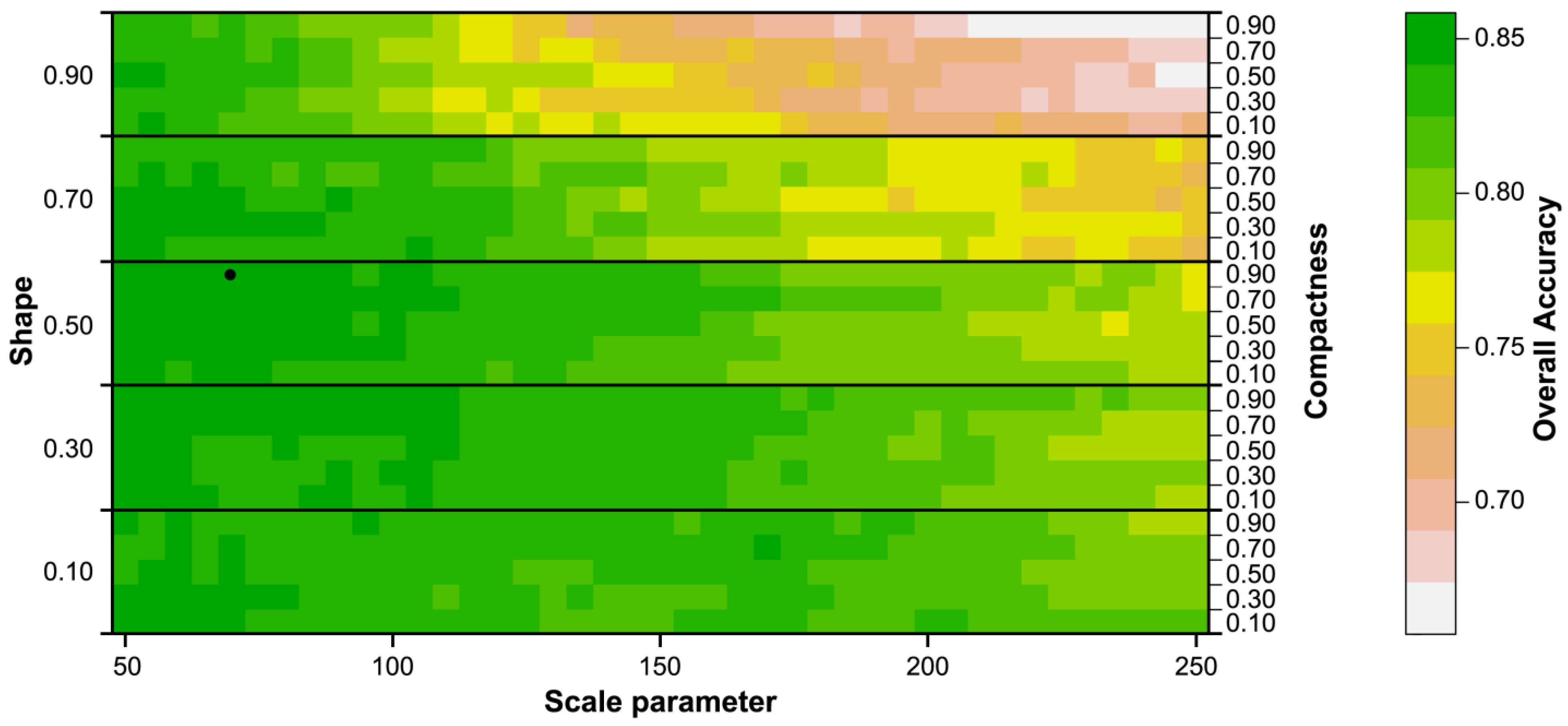
  • Classification results depend to a high degree on the identification of suitable segmentation parameters. In our study, the worst segmentation yielded an overall accuracy (OA) of only 0.66 compared to the best result with OA 0.86 (with kappa of 0.48 and 0.79, respectively). This large spread in classification accuracies underlines that procedures are needed for (automatically) choosing suitable parameter settings. Today, this is mostly done in a manual way (trial-and-error), not necessarily leading to the best possible result.
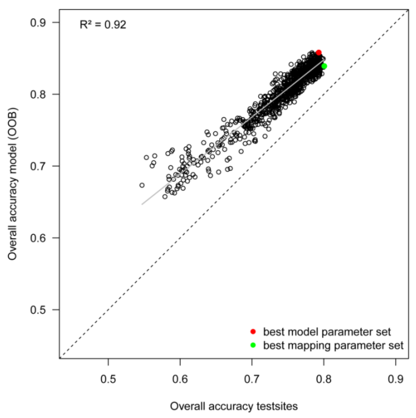
  • It is possible to fully automate the identification of suitable segmentation parameters (as well as input features for the classifier) using a full factorial design framework as chosen for this study (e.g., testing a pre-defined set of parameter combinations within fixed intervals each time optimizing input features using MDA information). The segmentation parameters derived from relatively few training samples were close to those one would have identified directly from another set of validation samples showing the robustness of the approach. The proposed optimization framework can be applied to all type of segmentation algorithms. Obviously, the simple feature selection approach chosen for our study can be replaced by other techniques. In our case, the resulting error surface (e.g., classification accuracy) was smooth enough to permit running a guided optimization procedure (Simplex or similar). It is not clear, however, if this would really speed-up the entire process.
  • For regions similar to the Assis study area with sub-tropical climate, soybean and sugarcane can be classified with acceptable accuracy using two Landsat scenes acquired in January/February and August. However, using such acquisition dates, it was not possible to correctly map cassava and (to a lesser extend) peanut. The spectral signatures of these two crops were too similar for permitting a successful discrimination and mapping. Additional information would be required to map peanut and cassava with acceptable accuracy. The added-value of additional scenes also from other satellite sensors (e.g., Sentinel-2) deserves being tested in future work. In our study, additional scenes could not be processed due to persistent cloud coverage during the vegetative period.
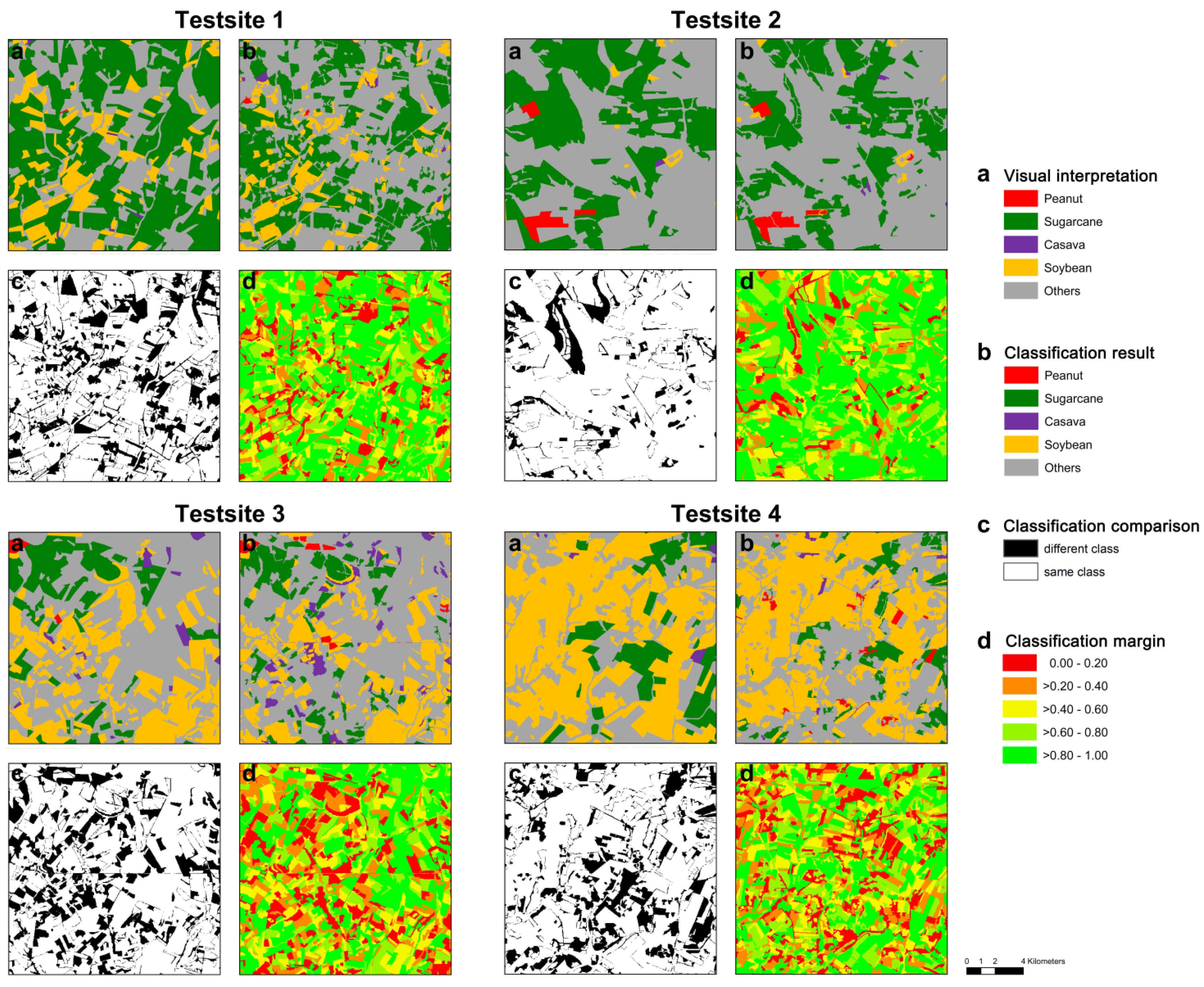
  • The classification margin—produced as a by-product using the Random Forest (RF) classifier—provides valuable information to the land cover (LC) map and deserves more attention. We were able to demonstrate (at pixel level) that the margin between first and second most often selected class (majority vote) closely reflects the accuracy of the final LC map. We found a close (linear) relation between the classification accuracy at pixel level and classification margin, with only 48% of the pixels being correctly classified in the worst case (margin <10%), while >92% of the pixels were correctly classified in the best case (margin >90%).
As part of the next steps, we plan to speed up the processing, for example, by using alternative segmentation algorithms (e.g., mean shift). In the same spirit, we will also investigate the usage of other texture features such as wavelets. Wavelets are known to considerably reduce processing time while providing information not present in GLCM. The highest time-savings can probably be achieved by optimizing the feature extraction for the segments. For this, a separation of the feature extraction part from the segmentation step is foreseen. Finally, we plan to compare the proposed method of supervised segmentation against unsupervised segmentation optimizations based on variance and Moran’s I. If both methods yield similar results, considerable savings in processing time could be realized. A speedup of processing would be highly welcome to take full advantage of upcoming satellite data such as Sentinel-2.

Acknowledgments

The authors are grateful for the funding provided through the INPE project (development and implementation of a satellite-based agricultural monitoring system for Brazil Project number 402.597/2012-5) within the Program “Science without Borders” from CNPq (National Council for Scientific and Technological Development). The authors are grateful to three anonymous reviewers who offered valuable recommendations and comments.

Author Contributions

All authors conceived and designed the study; Bruno Schulz, Antonio Roberto Formaggio did the field work and photo interpretation. Bruno Schulz and Markus Immitzer performed the data processing; Markus Immitzer, Bruno Schulz and Clement Atzberger analyzed the results; Bruno Schulz, Clement Atzberger and Markus Immitzer wrote the paper. Antonio R. Formaggio, Ieda D. Sanches and Alfredo J.B. Luiz revised the paper.

Conflicts of Interest

The authors declare no conflict of interest.

References

  1. Atzberger, C. Advances in remote sensing of agriculture: Context description, existing operational monitoring systems and major information needs. Remote Sens. 2013, 5, 949–981. [Google Scholar] [CrossRef]
  2. Becker-Reshef, I.; Justice, C.; Sullivan, M.; Vermote, E.; Tucker, C.; Anyamba, A.; Small, J.; Pak, E.; Masuoka, E.; Schmaltz, J.; et al. Monitoring global croplands with coarse resolution earth observations: The Global Agriculture Monitoring (GLAM) project. Remote Sens. 2010, 2, 1589–1609. [Google Scholar] [CrossRef]
  3. FAO. Food and Agriculture Organization of the United Nations—Statistics Division. Available online: http://faostat3.fao.org/browse/Q/QC/E (accessed on 10 May 2015).
  4. Arvor, D.; Meirelles, M.; Dubreuil, V.; Bégué, A.; Shimabukuro, Y.E. Analyzing the agricultural transition in Mato Grosso, Brazil, using satellite-derived indices. Appl. Geogr. 2012, 32, 702–713. [Google Scholar] [CrossRef]
  5. Arvor, D.; Jonathan, M.; Meirelles, M.S.P.; Dubreuil, V.; Durieux, L. Classification of MODIS EVI time series for crop mapping in the state of Mato Grosso, Brazil. Int. J. Remote Sens. 2011, 32, 7847–7871. [Google Scholar] [CrossRef]
  6. Ippoliti-Ramilo, G.A.; Epiphanio, J.C.N.; Shimabukuro, Y.E. Landsat-5 Thematic Mapper data for pre-planting crop area evaluation in tropical countries. Int. J. Remote Sens. 2003, 24, 1521–1534. [Google Scholar] [CrossRef]
  7. Rizzi, R.; Rudorff, B.F.T. Estimativa da área de soja no Rio Grande do Sul por meio de imagens Landsat. Rev. Bras. Cartogr. 2005, 3, 226–234. [Google Scholar]
  8. Sugawara, L.M.; Rudorff, B.F.T.; Adami, M. Viabilidade de uso de imagens do Landsat em mapeamento de área cultivada com soja no Estado do Paraná. Pesqui. Agropecuária Bras. 2008, 43, 1763–1768. [Google Scholar] [CrossRef]
  9. Vieira, M.A.; Formaggio, A.R.; Rennó, C.D.; Atzberger, C.; Aguiar, D.A.; Mello, M.P. Object Based Image Analysis and Data Mining applied to a remotely sensed Landsat time-series to map sugarcane over large areas. Remote Sens. Environ. 2012, 123, 553–562. [Google Scholar] [CrossRef]
  10. Rudorff, B.F.T.; Aguiar, D.A.; Silva, W.F.; Sugawara, L.M.; Adami, M.; Moreira, M.A. Studies on the rapid expansion of sugarcane for ethanol production in São Paulo State (Brazil) using Landsat data. Remote Sens. 2010, 2, 1057–1076. [Google Scholar] [CrossRef]
  11. Justice, C.O.; Townshend, J.R.G.; Vermote, E.F.; Masuoka, E.; Wolfe, R.E.; Saleous, N.; Roy, D.P.; Morisette, J.T. An overview of MODIS Land data processing and product status. Remote Sens. Environ. 2002, 83, 3–15. [Google Scholar] [CrossRef]
  12. Justice, C.O.; Vermote, E.; Townshend, J.R.G.; DeFries, R.; Roy, D.P.; Hall, D.K.; Salomonson, V.V.; Privette, J.L.; Riggs, G.; Strahler, A.; et al. The Moderate Resolution Imaging Spectroradiometer (MODIS): Land remote sensing for global change research. IEEE Trans. Geosci. Remote Sens. 1998, 36, 1228–1249. [Google Scholar] [CrossRef]
  13. Brown, J.C.; Kastens, J.H.; Coutinho, A.C.; de Castro Victoria, D.; Bishop, C.R. Classifying multiyear agricultural land use data from Mato Grosso using time-series MODIS vegetation index data. Remote Sens. Environ. 2013, 130, 39–50. [Google Scholar] [CrossRef]
  14. Galford, G.L.; Mustard, J.F.; Melillo, J.; Gendrin, A.; Cerri, C.C.; Cerri, C.E.P. Wavelet analysis of MODIS time series to detect expansion and intensification of row-crop agriculture in Brazil. Remote Sens. Environ. 2008, 112, 576–587. [Google Scholar] [CrossRef]
  15. Rembold, F.; Atzberger, C.; Savin, I.; Rojas, O. Using low resolution satellite imagery for yield prediction and yield anomaly detection. Remote Sens. 2013, 5, 1704–1733. [Google Scholar] [CrossRef] [Green Version]
  16. Lamparelli, R.A.; de Carvalho, W.M.; Mercante, E. Mapeamento de semeaduras de soja (Glycine max (L.) Merr.) mediante dados MODIS/Terra e TM/Landsat 5: um comparativo. Eng. Agríc. 2008, 28, 334–344. [Google Scholar] [CrossRef]
  17. Rudorff, C.M.; Rizzi, R.; Rudorff, B.F.T.; Sugawara, L.M.; Vieira, C.A.O. Spectral-temporal response surface of MODIS sensor images for soybean area classification in Rio Grande do Sul State. Ciênc. Rural 2007, 37, 118–125. [Google Scholar] [CrossRef]
  18. Yi, J.L.; Shimabukuro, Y.E.; Quintanilha, J.A. Identificação e mapeamento de áreas de milho na região sul do Brasil utilizando imagens MODIS. Eng. Agríc. 2007, 27, 753–763. [Google Scholar] [CrossRef]
  19. Luiz, A.J.B.; Epiphanio, J.C.N. Amostragem por pontos em imagens de sensoriamento remoto para estimativa de área plantada por município. Simpósio Bras. Sensoriamento Remoto 2001, 10, 111–118. [Google Scholar]
  20. Atzberger, C.; Formaggio, A.R.; Shimabukuro, Y.E.; Udelhoven, T.; Mattiuzzi, M.; Sanchez, G.A.; Arai, E. Obtaining crop-specific time profiles of NDVI: the use of unmixing approaches for serving the continuity between SPOT-VGT and PROBA-V time series. Int. J. Remote Sens. 2014, 35, 2615–2638. [Google Scholar] [CrossRef]
  21. Lobell, D.B.; Asner, G.P. Cropland distributions from temporal unmixing of MODIS data. Remote Sens. Environ. 2004, 93, 412–422. [Google Scholar] [CrossRef]
  22. Ozdogan, M. The spatial distribution of crop types from MODIS data: Temporal unmixing using Independent Component Analysis. Remote Sens. Environ. 2010, 114, 1190–1204. [Google Scholar] [CrossRef]
  23. Gao, F.; Masek, J.; Schwaller, M.; Hall, F. On the blending of the Landsat and MODIS surface reflectance: Predicting daily Landsat surface reflectance. IEEE Trans. Geosci. Remote Sens. 2006, 44, 2207–2218. [Google Scholar] [CrossRef]
  24. Hilker, T.; Wulder, M.A.; Coops, N.C.; Seitz, N.; White, J.C.; Gao, F.; Masek, J.G.; Stenhouse, G. Generation of dense time series synthetic Landsat data through data blending with MODIS using a spatial and temporal adaptive reflectance fusion model. Remote Sens. Environ. 2009, 113, 1988–1999. [Google Scholar] [CrossRef]
  25. Singh, D. Evaluation of long-term NDVI time series derived from Landsat data through blending with MODIS data. Atmósfera 2012, 25, 43–63. [Google Scholar]
  26. Wu, M.; Niu, Z.; Wang, C.; Wu, C.; Wang, L. Use of MODIS and Landsat time series data to generate high-resolution temporal synthetic Landsat data using a spatial and temporal reflectance fusion model. J. Appl. Remote Sens. 2012, 6, 063507–1. [Google Scholar]
  27. Cowen, D.J.; Jensen, J.R.; Bresnahan, P.J.; Ehler, G.B.; Graves, D.; Huang, X.; Wiesner, C.; Mackey, H.E. The design and implementation of an integrated geographic information system for environmental applications. Photogramm. Eng. Remote Sens. 1995, 61, 1393–1404. [Google Scholar]
  28. Powell, S.L.; Pflugmacher, D.; Kirschbaum, A.A.; Kim, Y.; Cohen, W.B. Moderate resolution remote sensing alternatives: A review of Landsat-like sensors and their applications. J. Appl. Remote Sens. 2007. [Google Scholar] [CrossRef]
  29. Whitcraft, A.K.; Becker-Reshef, I.; Killough, B.D.; Justice, C.O. Meeting earth observation requirements for global agricultural monitoring: An evaluation of the revisit capabilities of current and planned moderate resolution optical earth observing missions. Remote Sens. 2015, 7, 1482–1503. [Google Scholar] [CrossRef]
  30. Blaschke, T. Object based image analysis for remote sensing. ISPRS J. Photogramm. Remote Sens. 2010, 65, 2–16. [Google Scholar] [CrossRef]
  31. Duro, D.C.; Franklin, S.E.; Dubé, M.G. A comparison of pixel-based and object-based image analysis with selected machine learning algorithms for the classification of agricultural landscapes using SPOT-5 HRG imagery. Remote Sens. Environ. 2012, 118, 259–272. [Google Scholar] [CrossRef]
  32. Hay, G.J.; Castilla, G. Geographic Object-Based Image Analysis (GEOBIA): A new name for a new discipline. In Object-Based Image Analysis; Blaschke, T., Lang, S., Hay, G.J., Eds.; Lecture Notes in Geoinformation and Cartography; Springer: Berlin/Heidelberg, Germany, 2008; pp. 75–89. [Google Scholar]
  33. Löw, F.; Duveiller, G. Defining the spatial resolution requirements for crop identification using optical remote sensing. Remote Sens. 2014, 6, 9034–9063. [Google Scholar] [CrossRef]
  34. Myint, S.W.; Gober, P.; Brazel, A.; Grossman-Clarke, S.; Weng, Q. Per-pixel vs. object-based classification of urban land cover extraction using high spatial resolution imagery. Remote Sens. Environ. 2011, 115, 1145–1161. [Google Scholar] [CrossRef]
  35. Toscani, P.; Immitzer, M.; Atzberger, C. Texturanalyse mittels diskreter Wavelet Transformation für die objektbasierte Klassifikation von Orthophotos. Photogramm. Fernerkund. Geoinf. 2013, 2, 105–121. [Google Scholar] [CrossRef]
  36. Devadas, R.; Denham, R.J.; Pringle, M. Support vector machine classification of object-based data for crop mapping, using multi-temporal Landsat imagery. Int. Arch. Photogramm. Remote Sens. Spat. Inf. Sci. 2012, 39, 185–190. [Google Scholar] [CrossRef]
  37. Dronova, I.; Gong, P.; Clinton, N.E.; Wang, L.; Fu, W.; Qi, S.; Liu, Y. Landscape analysis of wetland plant functional types: The effects of image segmentation scale, vegetation classes and classification methods. Remote Sens. Environ. 2012, 127, 357–369. [Google Scholar] [CrossRef]
  38. Formaggio, A.R.; Vieira, M.A.; Renno, C.D. Object Based Image Analysis (OBIA) and Data Mining (DM) in Landsat time series for mapping soybean in intensive agricultural regions. In Proceedings of the IEEE International Geoscience and Remote Sensing Symposium (IGARSS), Munich, Germany, 22–27 July 2012; pp. 2257–2260.
  39. Formaggio, A.R.; Vieira, M.A.; Rennó, C.D.; Aguiar, D.A.; Mello, M.P. Object-Based Image Analysis and Data Mining for mapping sugarcane with Landsat imagery in Brazil. Int. Arch. Photogramm. Remote Sens. Spat. Inf. Sci. 2010, 38, 553–562. [Google Scholar]
  40. Long, J.A.; Lawrence, R.L.; Greenwood, M.C.; Marshall, L.; Miller, P.R. Object-oriented crop classification using multitemporal ETM+ SLC-off imagery and random forest. GIScience Remote Sens. 2013, 50, 418–436. [Google Scholar]
  41. Peña-Barragán, J.M.; Ngugi, M.K.; Plant, R.E.; Six, J. Object-based crop identification using multiple vegetation indices, textural features and crop phenology. Remote Sens. Environ. 2011, 115, 1301–1316. [Google Scholar] [CrossRef]
  42. Peña, J.M.; Gutiérrez, P.A.; Hervás-Martínez, C.; Six, J.; Plant, R.E.; López-Granados, F. Object-based image classification of summer crops with machine learning methods. Remote Sens. 2014, 6, 5019–5041. [Google Scholar] [CrossRef]
  43. Dey, V.; Zhang, Y.; Zhong, M. A review on image segmentation techniques with remote sensing perspective. Int. Arch. Photogramm. Remote Sens. Spat. Inf. Sci. 2010, 38, 31–42. [Google Scholar]
  44. Forster, D.; Kellenberger, T.W.; Buehler, Y.; Lennartz, B. Mapping diversified peri-urban agriculture—Potential of object-based versus per-field land cover/land use classification. Geocarto Int. 2010, 25, 171–186. [Google Scholar] [CrossRef]
  45. Muñoz, X.; Freixenet, J.; Cufı́, X.; Martı́, J. Strategies for image segmentation combining region and boundary information. Pattern Recognit. Lett. 2003, 24, 375–392. [Google Scholar] [CrossRef]
  46. Yan, L.; Roy, D.P. Automated crop field extraction from multi-temporal Web Enabled Landsat Data. Remote Sens. Environ. 2014, 144, 42–64. [Google Scholar] [CrossRef]
  47. Baatz, M.; Schäpe, A. Multiresolution Segmentation: An optimization approach for high quality multi-scale image segmentation. In Angewandte Geographische Informationsverarbeitung XII; Strobl, J., Blaschke, T., Griesebner, G., Eds.; Wichmann Verlag: Karlsruhe, Germany, 2000; pp. 12–23. [Google Scholar]
  48. Liu, D.; Xia, F. Assessing object-based classification: Advantages and limitations. Remote Sens. Lett. 2010, 1, 187–194. [Google Scholar] [CrossRef]
  49. Stumpf, A.; Kerle, N. Object-oriented mapping of landslides using Random Forests. Remote Sens. Environ. 2011, 115, 2564–2577. [Google Scholar] [CrossRef]
  50. Taşdemir, K.; Milenov, P.; Tapsall, B. A hybrid method combining SOM-based clustering and object-based analysis for identifying land in good agricultural condition. Comput. Electron. Agric. 2012, 83, 92–101. [Google Scholar] [CrossRef]
  51. Benz, U.C.; Hofmann, P.; Willhauck, G.; Lingenfelder, I.; Heynen, M. Multi-resolution, object-oriented fuzzy analysis of remote sensing data for GIS-ready information. ISPRS J. Photogramm. Remote Sens. 2004, 58, 239–258. [Google Scholar] [CrossRef]
  52. Bo, S.; Ding, L.; Li, H.; Di, F.; Zhu, C. Mean shift-based clustering analysis of multispectral remote sensing imagery. Int. J. Remote Sens. 2009, 30, 817–827. [Google Scholar] [CrossRef]
  53. Comaniciu, D.; Meer, P. Mean shift: A robust approach toward feature space analysis. IEEE Trans. Pattern Anal. Mach. Intell. 2002, 24, 603–619. [Google Scholar] [CrossRef]
  54. Beucher, S. The watershed transformation applied to image segmentation. Scanning Microsc. Suppl. 1992, 6, 299–299. [Google Scholar]
  55. Vantaram, S.R.; Saber, E. Survey of contemporary trends in color image segmentation. J. Electron. Imaging 2012. [Google Scholar] [CrossRef]
  56. Oliveira, J.C.; Formaggio, A.R.; Epiphanio, J.C.N.; Luiz, A.J.B. Index for the Evaluation of Segmentation (IAVAS): An application to agriculture. Mapp. Sci. Remote Sens. 2003, 40, 155–169. [Google Scholar] [CrossRef]
  57. Stefanski, J.; Mack, B.; Waske, B. Optimization of object-based image analysis with random forests for land cover mapping. IEEE J. Sel. Top. Appl. Earth Obs. Remote Sens. 2013, 6, 2492–2504. [Google Scholar] [CrossRef]
  58. IBGE Sistema IBGE de Recuperação Automática. Available online: http://www.sidra.ibge.gov.br (accessed on 8 March 2015).
  59. Alvares, C.A.; Stape, J.L.; Sentelhas, P.C.; de Moraes Gonçalves, J.L.; Sparovek, G. Köppen’s climate classification map for Brazil. Meteorol. Z. 2013, 22, 711–728. [Google Scholar] [CrossRef]
  60. Aguiar, D.A.; Rudorff, B.F.T.; Silva, W.F.; Adami, M.; Mello, M.P. Remote sensing images in support of environmental protocol: Monitoring the sugarcane harvest in São Paulo State, Brazil. Remote Sens. 2011, 3, 2682–2703. [Google Scholar] [CrossRef]
  61. De Aguiar, D.A.; Rudorff, B.T.F.; Rizzi, R.; Shimabukuro, Y.E. Monitoramento da colheita da cana-de-açúcar por meio de imagens MODIS. Rev. Bras. Cartogr. 2008, 4, 375–383. [Google Scholar]
  62. IEA Intituto de economia agricola: Área e Produção de milho de primeira safra, de segunda safra e irrigado, em 2014, no estado de São Paulo. Available online: http://ciagri.iea.sp.gov.br/nia1/ (accessed on 8 March 2015).
  63. Roy, D.P.; Wulder, M.A.; Loveland, T.R.; Woodcock, C.E.; Allen, R.G.; Anderson, M.C.; Helder, D.; Irons, J.R.; Johnson, D.M.; Kennedy, R.; et al. Landsat-8: Science and product vision for terrestrial global change research. Remote Sens. Environ. 2014, 145, 154–172. [Google Scholar] [CrossRef]
  64. Cihlar, J. Land cover mapping of large areas from satellites: Status and research priorities. Int. J. Remote Sens. 2000, 21, 1093–1114. [Google Scholar] [CrossRef]
  65. INPE. Available online: http://cbers2.dpi.inpe.br/ (accessed on 8 March 2015).
  66. Sanches, I.D.; Epiphanio, J.C.N.; Formaggio, A.R. Culturas agrícolas em imagens multitemporais do satélite Landsat. Agric. Em São Paulo 2005, 52, 83–96. [Google Scholar]
  67. Breiman, L. Random forests. Mach. Learn. 2001, 45, 5–32. [Google Scholar] [CrossRef]
  68. Immitzer, M.; Atzberger, C.; Koukal, T. Tree species classification with Random Forest using very high spatial resolution 8-band WorldView-2 satellite data. Remote Sens. 2012, 4, 2661–2693. [Google Scholar] [CrossRef]
  69. Pal, M. Random forest classifier for remote sensing classification. Int. J. Remote Sens. 2005, 26, 217–222. [Google Scholar] [CrossRef]
  70. Rodríguez-Galiano, V.F.; Chica-Olmo, M.; Abarca-Hernandez, F.; Atkinson, P.M.; Jeganathan, C. Random Forest classification of Mediterranean land cover using multi-seasonal imagery and multi-seasonal texture. Remote Sens. Environ. 2012, 121, 93–107. [Google Scholar] [CrossRef]
  71. Waske, B.; Braun, M. Classifier ensembles for land cover mapping using multitemporal SAR imagery. ISPRS J. Photogramm. Remote Sens. 2009, 64, 450–457. [Google Scholar] [CrossRef]
  72. Immitzer, M.; Atzberger, C. Early Detection of Bark Beetle Infestation in Norway Spruce (Picea abies, L.) using WorldView-2 Data. Photogramm. Fernerkund. Geoinf. 2014, 2014, 351–367. [Google Scholar] [CrossRef]
  73. Breiman, L. Manual on Setting up, Using, and Understanding Random Forests V3.1; University of California at Berkeley: Berkeley, CA, USA, 2002. [Google Scholar]
  74. Hastie, T.; Tibshirani, R.; Friedman, J. The Elements of Statistical Learning: Data Mining, Inference, and Prediction, 2nd ed.; Springer: New York, NY, USA, 2009. [Google Scholar]
  75. Guyon, I.; Weston, J.; Barnhill, S.; Vapnik, V. Gene selection for cancer classification using support vector machines. Mach. Learn. 2002, 46, 389–422. [Google Scholar] [CrossRef]
  76. Vuolo, F.; Atzberger, C. Improving land cover maps in areas of disagreement of existing products using NDVI time series of MODIS—Example for Europe. Photogramm. Fernerkund. Geoinf. 2014, 2014, 393–407. [Google Scholar] [CrossRef]
  77. R Core Team. R: A Language and Environment for Statistical Computing; R Foundation for Statistical Computing: Vienna, Austria, 2015. [Google Scholar]
  78. Liaw, A.; Wiener, M. Classification and regression by randomForest. R News 2002, 2, 18–22. [Google Scholar]
  79. Hijmans, R.J. Raster: Geographic Data Analysis and Modeling R package. 2014.
  80. Kuhn, M.; Wing, J.; Weston, S.; Williams, A.; Keefer, C.; Engelhardt, A.; Cooper, T.; Mayer, Z. Caret: Classification and Regression Training R package. 2014.

