Mapping Cropping Practices of a Sugarcane-Based Cropping System in Kenya Using Remote Sensing

Abstract

Over the recent past, there has been a growing concern on the need for mapping cropping practices in order to improve decision-making in the agricultural sector. We developed an original method for mapping cropping practices: crop type and harvest mode, in a sugarcane landscape of western Kenya using remote sensing data. At local scale, a temporal series of 15-m resolution Landsat 8 images was obtained for Kibos sugar management zone over 20 dates (April 2013 to March 2014) to characterize cropping practices. To map the crop type and harvest mode we used ground survey and factory data over 1280 fields, digitized field boundaries, and spectral indices (the Normalized Difference Vegetation Index (NDVI) and the Normalized Difference Water Index (NDWI)) were computed for all Landsat images. The results showed NDVI classified crop type at 83.3% accuracy, while NDWI classified harvest mode at 90% accuracy. The crop map will inform better planning decisions for the sugar industry operations, while the harvest mode map will be used to plan for sensitizations forums on best management and environmental practices.

1. Introduction

International agreements like the Rio Convention, as well as national legislation and regional policies, require the management of rural areas both for agricultural production and for other uses (reduction of greenhouse gas emission, carbon sequestration, biodiversity conservation, etc.) on a large scale. The last decade has seen the rapid development of research on the topic of ecosystem services and, increasing awareness of the economic value of ecosystem goods and services among decision-makers. Remotely sensed data offers a unique opportunity to provide environmental information with complete coverage, at different spatial and temporal resolutions. A key advantage of remote sensing is the capability to perform synoptic, spatially continuous and frequent observations resulting in large data volumes and multiple datasets at varying spatial and temporal resolutions [1].

Farming practices directly affect the provision of ecosystem services. Mapping these practices is thus a challenge both for researchers in agro-ecology and decision-makers. Tillage systems for instance drastically impact on greenhouse gas emission by agriculture [2], and influence the development of classification method for mapping tillage practices at a regional scale [3]. In the case of sugar cane, mulching crop residues at harvest, instead of burning it, significantly contributes to sustained land productivity, increased organic matter in soils [4], and decrease in greenhouse-gas emission [5,6].

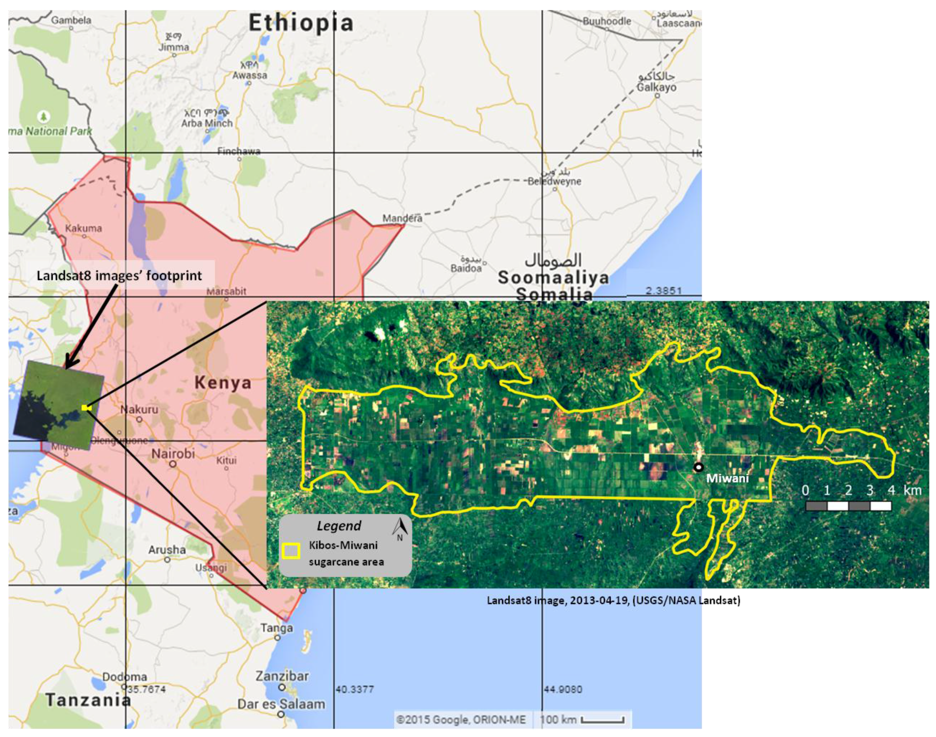
The sugarcane landscape in Kenya is composed of small-scale farmers (below five hectares (ha)) whose land is heavily fragmented and large-scale farmers (over 5 ha), with both sugarcane and food crops in respective agronomic fields and a diversified crop calendar. A baseline survey by KESREF [7] revealed that the minimum agronomic field size for a small scale holder was 0.2 ha with more than three food crops in the farm associated with high levels of crop rotation. Variability in crop type introduces variations in crop residues and harvest type within the same landscape. Characterizing cropping practices (type of crop and harvest mode) in such heterogeneous fields is thus important to ensure that information on cropping practices at field level is identified for enhanced planning of sugarcane census, harvesting and transport operations [8]. We proposed to identify suitable remote sensing indices to map cropping practices (crop type and harvest mode) in a complex agricultural landscape in Kenya, based on free remote sensing images. Mapping cropping practices for the sugarcane landscape in Kenya will be crucial in providing area under sugarcane crop. Area under sugarcane is a critical function of the yearly cane census [9] which is a key input in the planning process. The sugar industry therefore requires spatially explicit tools to provide reliable and precise information on area under sugarcane and location of sugarcane fields to improve accuracy in monitoring sugarcane production and yield estimates [8,10]. Moreover, in a landscape where 85% of sugarcane is grown among other land uses, mapping of cropping practices is vital in ensuring improved planning and management of the diversified natural resources. Additionally, mapping of cropping practices in a landscape that is diverse in topography is difficult especially where the spatial and temporal information of these practices is required unless modern tools are utilized.

Until today, mapping sugarcane acreage in Kenya is undertaken using manual methods while utilizing the theodolites and tape measure. This method although acceptable by the geospatial fraternity, is tedious, usually associated with disadvantages that accrue from manual methods such as; gross error, high costs for retaining officers in the fields and long periods that the exercise takes to complete, which contribute to inaccuracy in real time representation [11]. Physical methods for such mapping approaches only capture spatial extend for accessible areas [12]. Except the crop suitability maps in existence today, there are no maps showing the sugarcane cropped fields and/or harvest mode in Kenya and this constrains planning for farm inputs such as fertilizer distribution by the government. Moreover, inaccessibility of certain areas in the landscape reduces accuracy in physical approaches. It is therefore important to present precise estimations of such acreage using modern tools that are able to capture both temporal and spatial variations in sugarcane area that accrue from crop cycles and expansion of this production area.

Remote sensing data is sensitive to the land surface components (water, vegetation, soil) which can be used to map land cover, subsequently describing surface type and conditions in every point of space, on regular basis [13]. Remote sensing imagery, when converted into useful information and integrated with data from geographical information systems (GIS), can increase accuracy in monitoring spatial and temporal dynamics as well as crop development [10], and provide area measurements. Recent studies have used remote sensing images to map sugarcane fields through automatic classification of Landsat images [14], through a rule-based classifier applied to SPOT image time series [15] or through an object based image analysis (OBIA) approach on high resolution image time series [16] to categorize sugarcane fields into similar age units. In countries where sugarcane is distributed over large areas and in large fields, like in Brazil, Thenkabail et al. [17] suggested the need for automated methods to map sugarcane fields and other land uses using time series Moderate Resolution Imaging Spectroradiometer (MODIS) 250 m images, coupled with Landsat 30 m images.

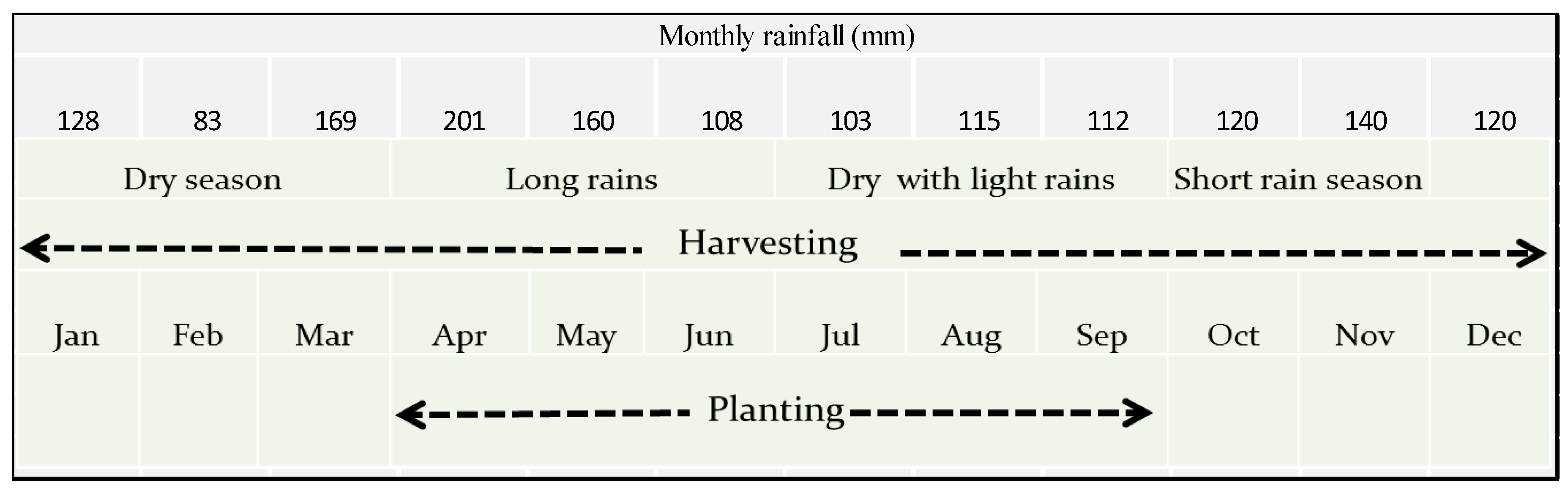
In Kenya where sugarcane fields are small, 30 m Landsat image can be useful in locating sugarcane fields of similar age. In the recent past, Landsat 30 m Normalized Difference Vegetation Index (NDVI) has facilitated exploration of the spatial variability of heterogeneous landscapes [18]. However, the multiple planting and harvesting calendar [19] in Kenya complicates land use mapping, necessitating the need for temporal series of satellite images for identification of which fields contain sugarcane [13,20]. The combination of varied spatial resolutions and temporal satellite images in mapping such fields minimizes inaccuracies in mapping disparate fields from a single image. To a large extend, although the Kenya sugar industry prohibits burnt cane harvesting because it depletes soil nutrients [21], this practice is still rampant in sub humid agro-ecological zones and on small scales in humid areas, usually being attributed to the need to maximize on harvested stalk [22]. Moreover, if burnt stalk is not harvested and milled within 48 h, the sucrose is usually destroyed, limiting the possibility to extract sugar that is already produced in deficit for the nation’s demand [8]. Characterizing this harvest mode is therefore important for improved decision-making, planning for harvesting operations and enhanced sugarcane productivity. In Brazil, the MODIS images facilitated detection of sugarcane harvest and harvest mode using the Normalized Difference Vegetation Index (NDVI) [23]. Lebourgeois et al. 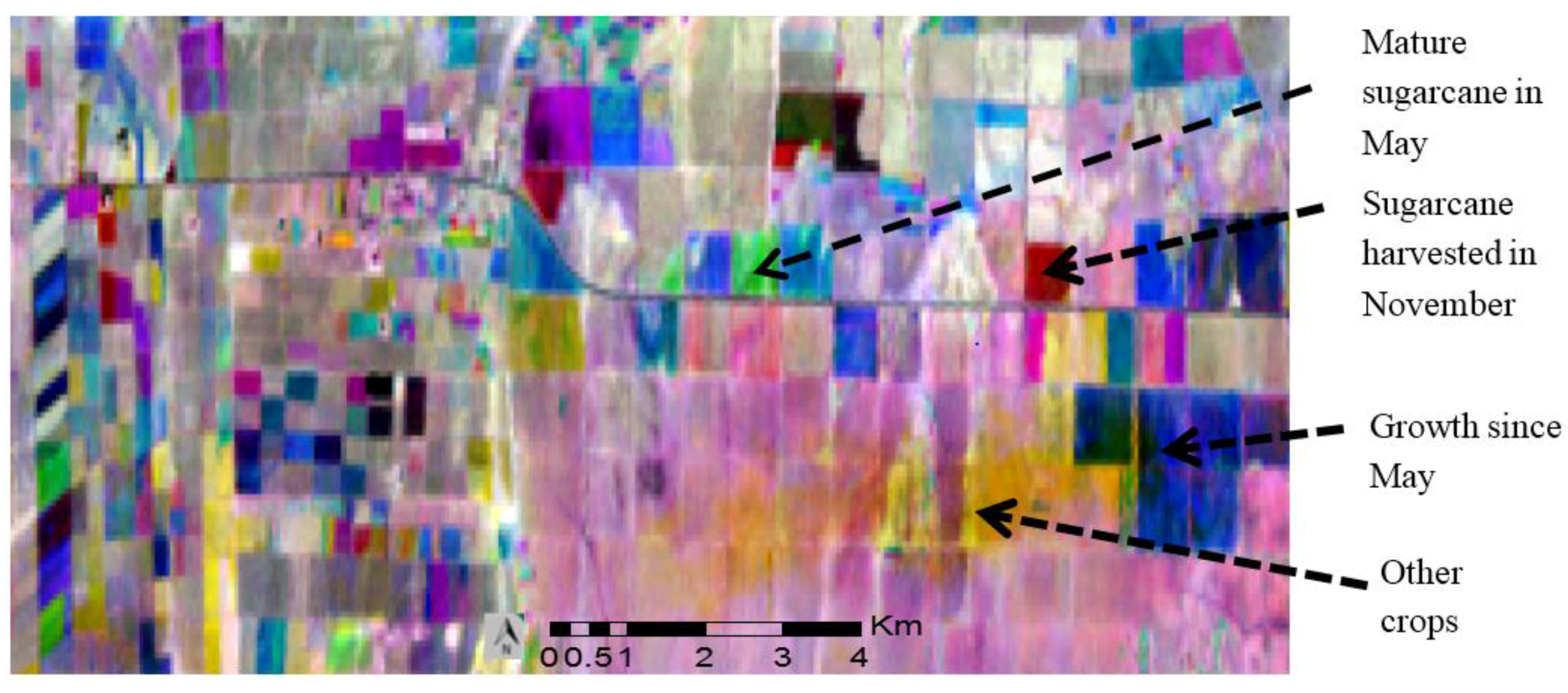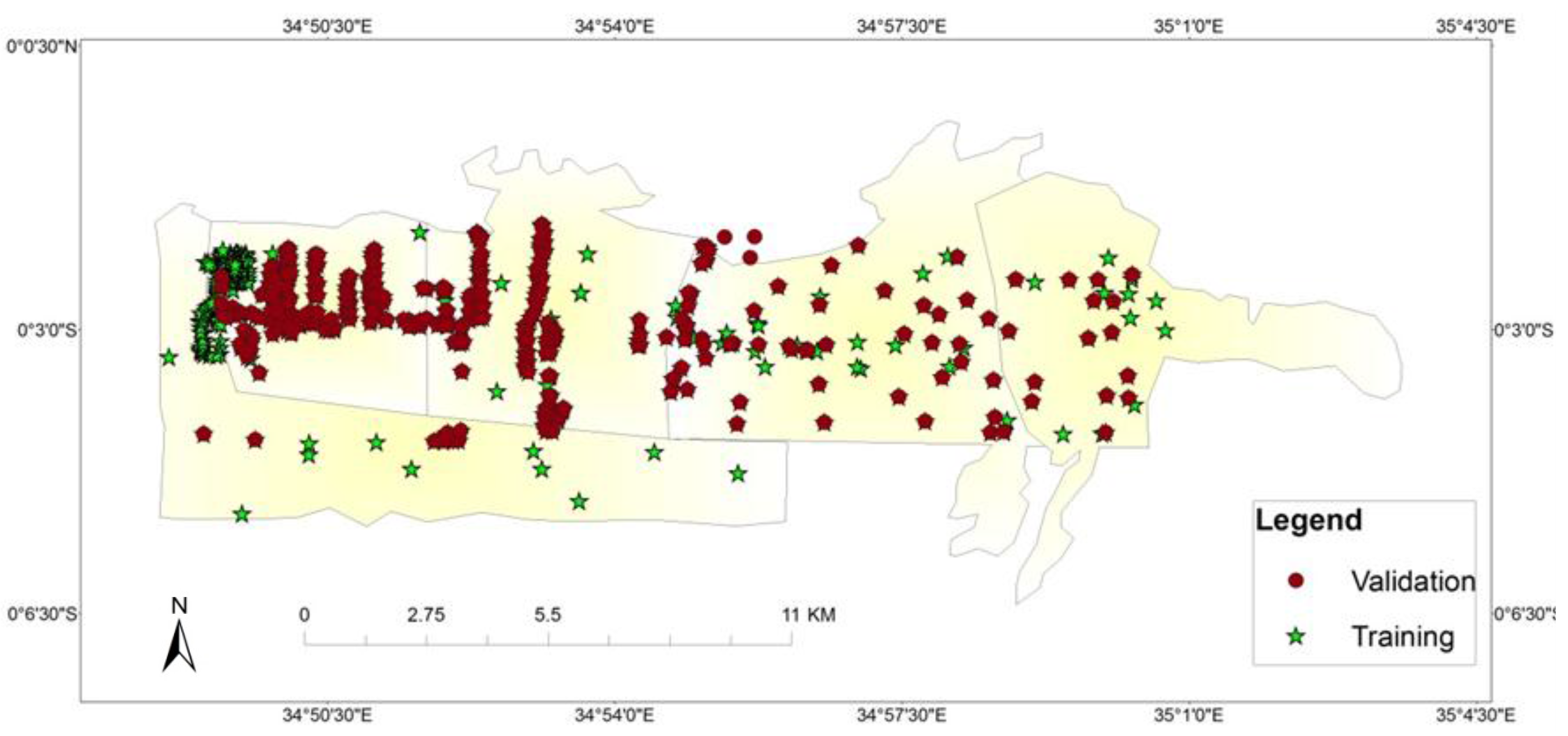[24] showed that the signal measured in the Short Wave InfraRed band (SWIR) was a good indicator of the presence of sugarcane harvest residues on the ground. Production area in western Kenya, displays a heterogeneous landscape due to different crop types, different cropping calendars and sugarcane harvest mode. Because of its ability to distinguish fields with sugarcane from other crops through time and different cropping practices, we used a complete year time series of Landsat8 images to develop an original method for mapping the spatial and temporal dynamics in the landscape; and ground data for classification training and validation.

2. Material and Methods

2.1. Study Area

The study covers Kibos-Miwani sugarcane zone in Kenya (Figure 1) at a local landscape scale within a space of 104 km² and located between 34.8°E to 35.08°E and 0.01°S to 0.11°S. The area has an altitude of 1000 m above sea level, receiving rainfall of between 1400 mm and 1550 mm and an average size of land measuring 3 hectares (ha). The main crop in the zone is sugarcane, besides maize and horticultural crops. Different sugarcane varieties are planted in the months of April and September congruent with the bimodal rainfall in March to June and September to December [9,25]. According to KESREF surveys of October 2013, harvesting of this crop is either by burning (over 70%) before cutting the stalks or by green harvest modes (cutting with trash). It is the diversified planting dates and different harvesting modes that provide an enabling environment to undertake mapping of cropping practices (crop type and harvest mode) in this zone.

Figure 1. Location of Kibos-Miwani sugar zone (Data source: ©2015 Google, USGS/NASA Landsat).

Figure 1. Location of Kibos-Miwani sugar zone (Data source: ©2015 Google, USGS/NASA Landsat).

2.2. Data

2.2.1. Ground Survey Data

Figure 2 illustrates the monthly rainfall, cropping calendar and harvesting culture. Planting is undertaken between April and September due to the bimodal rainfall received in western Kenya [19], maturity lasts between 14 and 18 months, while harvesting is conducted throughout the year depending on rainfall, variety and crop cycle (plant crop (for first planted crop) or ratoon (regrowth after each harvest since sugarcane is a perennial crop)). It is observed that planting occurs during the month with increased rainfall.

Figure 2. Sugarcane cropping calendar in western Kenya.

Figure 2. Sugarcane cropping calendar in western Kenya.

The choice of variety to plant depends on availability of seed cane within the agro-ecological zone. Well-managed ratoon crops exceed three cycles depending on sugarcane yield and influence of the miller on contracted farmers. During the planting season, other food crops are also planted which mature within a maximum of six months. The continuous harvesting is aimed at providing a regular supply of sugarcane to the factories throughout the year and minimizing cane surplus that the milling capacity of factories may not handle.

Cropping practices: Random sampling was used to collect data on cropping practices in Kibos-Miwani zone using a questionnaire for oral interview and the differential global positioning system (DGPS) for encoding the central positions of fields for interviewed farmers. During the survey, 384 farmers were interviewed based on a random sample of the population size of 4000 farmers. This number of sampled farmers was calculated according to [26] formula that was developed for selecting a representative sample in an investigation from large populations:

n₀ = Z² p q/e²

(1)

where

• n₀ = sample size;
• Z² = abscissa of the normal curve that cuts off an area of desired confidence level at the tails;
• e = desired level of precision;
• p = maximum variability of farmers that will be studied;
• q = 1 − p.

In this study, Z = 1.96 (for 95%); e = 0.05, p = 0.5, q = 0.5; leading to a theoretical number n₀ of 384 farmers to be interviewed.

In total, 1280 fields (800 sugarcane fields and 480 other land cover) belonging to this set of farmers (located by the GPS) were used to create the three following datasets: land cover type (sugarcane or other), planting and harvesting dates, and mode of harvesting. The “other” land cover referred to in this study consist of other crops, natural vegetation (shrubs and pasture), roads and buildings. These data were collected during a ground survey conducted in October 2013, and from Kibos Sugar Factory database:

-

The ground survey data were composed of 831 observations, where 530 fields were sugarcane and 301 fields were other land cover. These fields were encoded during a ground survey conducted between 14 and 18 October 2013. Figure 3 illustrates the location of the surveyed fields in Kibos-Miwani zone, showing location of those used for training (75%) and those used for validation (25%).

-

The Kibos Sugar Factory database was composed of 449 fields, where 270 fields were sugarcane fields and 179 fields were other land cover. These data were adopted from the existing land use data set compiled on 15 August 2013 by Kibos Sugar factory. Attributes for these fields (planting and harvesting date) were entered in our database in accordance with the factory office record. The factory data was relevant since it was collected within the study time frame of this research.

Figure 3. Ground survey points collected in Kibos-Miwani. The field survey was conducted from 14 to 18 October 2013. Seventy-five percent of the points were used for land use classification training the other 25% were used for classification validation.

Figure 3. Ground survey points collected in Kibos-Miwani. The field survey was conducted from 14 to 18 October 2013. Seventy-five percent of the points were used for land use classification training the other 25% were used for classification validation.

2.2.2. Satellite Data and Preprocessing

A complete one-year time series (April 2013–March 2014) of 20 Landsat 8 Operational Land Imager (OLI) images were downloaded through the online Data Pool at the NASA Land Processes Distributed Active Archive Center (LP DAAC: https://lpdaac.usgs.gov/get_data). Landsat 8 products consist of nine spectral bands with a spatial resolution of 30 m for Bands 2 to 9. The resolution for Band 8 (panchromatic) is 15 m and was used to enhance field boundaries. Approximate scene size is 170 km north–south by 183 km east–west. Table 1 summarizes Landsat 8 bands that were used in this study. The images were acquired orthorectified and geo-referenced in WGS84 UTM zone 36S.

Table 1. Landsat 8 Operational Land Imager (OLI) bands used in this study.

Bands	Wavelength (micrometers)	Resolution (m)
Band 4–Red	0.64–0.67	30
Band 5-Near Infrared (NIR)	0.85–0.88	30
Band 6-ShortWave InfraRed (SWIR 1)	1.57–1.65	30
Band 8-Panchromatic	0.50–0.68	15

Table 1. Landsat 8 Operational Land Imager (OLI) bands used in this study.

Bands	Wavelength (micrometers)	Resolution (m)
Band 4–Red	0.64–0.67	30
Band 5-Near Infrared (NIR)	0.85–0.88	30
Band 6-ShortWave InfraRed (SWIR 1)	1.57–1.65	30
Band 8-Panchromatic	0.50–0.68	15

2.3. Methods

2.3.1. Landsat 8 Image Analysis

Image processing was performed using ERDAS Imagine® (Intergraph Corp.: Norcross, GA USA).

Subset of the Landsat image, and band selection (Red, NIR and SWIR) was performed based on the extent of the study area. The multispectral bands were merged with the panchromatic band using the Brovey transform algorithm resulting in multispectral images at 15 m spatial resolution. Cloud and cloud shadow masks were then prepared based on the grow properties drawing tool that was able to trace out areas covered with clouds and shadows.

Two vegetation indices were derived using the following formula [27,28]:

NDVI = (NIR–RED)/(NIR + RED) [27]

(2)

NDWI = (SWIR–NIR)/(SWIR + NIR) [28]

(3)

The NDVI (Normalized Difference Vegetation Index), which is the normalized difference between the near infrared (NIR) and visible RED reflectance, is responsive to changes in vegetation cover and greenness. Higher NDVI values reflect greater vigor and photosynthetic capacity (or greenness) of dense vegetation canopy, whereas low NDVI values are reflective of vegetative stress or senescence, or low vegetation cover.

The NDWI (Normalized Difference Water Index), derived from the NIR and shortwave Infrared (SWIR) channels, responds to changes in both the water content (absorption of SWIR radiation) and structure (reflectance of NIR radiation) in vegetation canopies, respectively. In a different study, SWIR index was used in detection of a harvest because it separates harvested residues from any other crop status [24]. In this study, the SWIR band is used to compute the NDWI index due to its ability to detect moisture conditions of vegetation over large areas [29].

A map layer showing the limits of agronomic fields was digitized from the 15 m multispectral Landsat 8 image of 19 April 2013, in ArcGIS 10.1 software. The points encoded during the survey were added to this digitized layer. NDVI and NDWI images were sequentially stacked to generate two images of 20 layers each (20 dates between April 2013 to March 2014). The median and standard deviation of these time series values were then extracted for each digitized field using the zonal attribute function. Cloud pixels were set to 0, and were not taken into account in the statistics.

2.3.2. Mapping Cropping Practices

Cropping practices (in this document) imply the crop type and sugarcane harvest mode. To understand the spatial and spectral variability of the land cover types and crop conditions (type of crop, harvest mode), the two following analysis were performed: (1) true color composites of different sets of Landsat 8 images were examined for color, pattern, shape, and texture to visualize and interpret the land cover type and detect a harvest; and (2) the temporal variations of NDVI and NDWI were analyzed to identify the best index to detect crop type and harvest mode in Kibos-Miwani.

A map for sugarcane was produced using the temporal stack of NDVI images, following [30] methodology, extracted from the 20 Landsat NDVI images with assumption that NDVI time series was a good descriptor of land cover type. This approach captures sugarcane fields of different ages from temporal series, hence diminishes inaccuracies in mapping disparate fields from a single image that would classify harvested fields as bare land.

Sugarcane crop is highly variable in space because of diverse planting and harvesting dates; and variable crop cycles therefore we processed the classification map in two steps:

First, the Landsat time series was classified using ground survey points (composed of type of crop, harvest type and harvest date) and a supervised classification into five classes of “sugarcane” at different ages, and one class of “other” (Table 2), using a maximum likelihood classifier algorithm. The six characterized units were assigned class names based on field surveyed attributes. Seventy-five percent of the 1280 data points (960 points, where 600 were sugarcane and 360 were other land cover) were used as training data identify each thematic class, while 25% of the data (320, where 200 were sugarcane and 120 were other land cover points from the ground survey) were used for validation of the classified map.

Table 2. Distribution of survey points used in classification of five of “sugarcane” classes at different ages, and one class of “other”.

Class Name	Age (Months)	Number of Points
Sugarcane #1	0–2	131
Sugarcane #2	3–5	129
Sugarcane #3	6–8	150
Sugarcane #4	9–11	100
Sugarcane #5	Over 12	90
Other	--	360
All	--	960

Table 2. Distribution of survey points used in classification of five of “sugarcane” classes at different ages, and one class of “other”.

Class Name	Age (Months)	Number of Points
Sugarcane #1	0–2	131
Sugarcane #2	3–5	129
Sugarcane #3	6–8	150
Sugarcane #4	9–11	100
Sugarcane #5	Over 12	90
Other	--	360
All	--	960

Secondly, post-classification was conducted by recoding and management of the assigned classes (five sugarcane classes and “other”) through the spatial analyst tool of the ArcGIS software based on the majority filter criteria. This resulted into one sugarcane class, and “other land cover” class, which formed the sugarcane map for Kibos-Miwani.

We investigated the best index for characterizing the harvest mode. For each surveyed field, we used the field data on harvest date and harvest mode to compute differences in NDWI and NDVI between each two dates for the 20 image dates. First, we assumed that the highest change in NDVI and NDWI occurs at harvest. Therefore, for each surveyed field we computed NDVI and NDWI difference in values before and after the harvest, for both burnt and green harvest fields separately. Secondly, we checked the significance of the NDVI and NDWI differences for the burnt and green harvested fields using a t-test. Further, we plotted the frequency of occurrence of the most significant spectral variable at 99% confidence level and fitted the plots with a Gaussian model to check for the threshold value that distinguishes between burnt and green harvest.

The accuracy of the classified image is assessed by comparing the classified map with the reference map. Moreover, accuracy assessment provides information on the product quality and identifies probable sources of errors. A confusion matrix is a standardized method to represent the accuracy of classification results derived from remote sensed data by calculating accuracy measurements which include [31]: overall accuracy, producer’s accuracy (number of pixels of the classification class/total pixels in the ground class), user’s accuracy ( number of correct pixels of the sampled class/total pixels in the classification class), the omission error (1-Producer’s Accuracy), and the commission error (1-User’s Accuracy).

-

For the sugarcane map, we evaluated accuracy of the classification by creating a confusion matrix based on the 25% of the unused ground data (320 points).

-

For the harvest mode map, we evaluated accuracy of the classification by creating a confusion matrix based on the 25% of the unused ground data (200 points).

3. Results and Discussion

3.1. Spatial Variability

A color-composition of 15 m NDVI Landsat images is displayed in Figure 4 showing varied cropping practices such as fields with young crop whose germination commenced in May, those harvested in November, mature crop that is due for harvest and other cover crops within Kibos-Miwani. These results have revealed multiple planting and harvesting dates at pixel level, between fields in the area with different types of crops, vegetated and harvested fields exemplified on the image composite. In this study, the variable NDVI pattern in different fields is an indicator of different types and ages of crops in the area where environmental conditions such as the dry season may affect mature crops thereby reducing their NDVI. This finding complements the cropping calendar of Kibos-Miwani, where food crops are planted during the same period as sugarcane. Vintrou et al [32] also found that low NDVI may indicate start of growth season, for young crop, or for crop of higher age, low NDVI may depict crop stress or start of maturation. Landsat 8 images have demonstrated spatial variability in vegetation conditions at the pixel scale with vegetated, harvested, planted fields and natural vegetation being identified on the image composite for the selected months. We assert that these cropping practices are the main driver of these local variations.

Figure 4. Landsat 8 NDVI colored composite image (R: May 2013; G: September 2013; B: November 2013). The image is located at 34°30′E–35°E and 0°S–0°45′S.

Figure 4. Landsat 8 NDVI colored composite image (R: May 2013; G: September 2013; B: November 2013). The image is located at 34°30′E–35°E and 0°S–0°45′S.

3.2. Sugarcane Classification

The NDVI image was used in characterization of the land cover map. Figure 5 shows a classified NDVI image of Kibos-Miwani into six classes. Five classes are “sugarcane” that results from variation in sugarcane age and one for “other” class (Table 3).

Figure 6 is zoomed-in area “A” of Figure 5, showing the high spatial heterogeneity in the landscape.

Figure 5. The classified Landsat image of Kibos-Miwani showing six land cover classes: five classes of “Sugarcane” based on different stages (represented by #) of the crop, and one class of “Other”.

Figure 5. The classified Landsat image of Kibos-Miwani showing six land cover classes: five classes of “Sugarcane” based on different stages (represented by #) of the crop, and one class of “Other”.

Table 3. Confusion matrix of the classified Landsat image for Kibos-Miwani (after post-classification). The overall accuracy is in bold.

--		Classification
		Sugarcane	Other	Unclassified	Line Total	Producer’s Accuracy	Omission Error
Ground Truth	Sugarcane	160	22	18	200	80.0%	20.0%
	Other	7	108	5	120	90.0%	10.0%
	Row total	167	130	23	320	--	--
	User’s accuracy	95.8%	83.1%	--	--	83.8%	--
	Commission error	4.2%	16.9%	--	--	--	--

Table 3. Confusion matrix of the classified Landsat image for Kibos-Miwani (after post-classification). The overall accuracy is in bold.

--		Classification
		Sugarcane	Other	Unclassified	Line Total	Producer’s Accuracy	Omission Error
Ground Truth	Sugarcane	160	22	18	200	80.0%	20.0%
	Other	7	108	5	120	90.0%	10.0%
	Row total	167	130	23	320	--	--
	User’s accuracy	95.8%	83.1%	--	--	83.8%	--
	Commission error	4.2%	16.9%	--	--	--	--

The spatial heterogeneity between sugarcane fields in Figure 6 is assumed to imply that crop management such as planting date, weed control, harvesting mode are the drivers of these local variations [7,18]. Figure 7 shows the classified Landsat image of Kibos-Miwani after post classification. The figure illustrates two classes, sugarcane and other, and shows that over 85% of the landscape is under sugarcane.

A majority filter was then applied on the classified image in Figure 7 to enhance boundaries for the two classes (Figure 8). Spatial variability deplored in the fields is a confirmation to results of a study that showed that sugarcane landscapes are spatially heterogeneous due to variable cropping practices [18,33].

Figure 6. A zoom on the classified Landsat image of Kibos-Miwani sugar zone in area “A”.

Figure 6. A zoom on the classified Landsat image of Kibos-Miwani sugar zone in area “A”.

Figure 7. A classified Landsat image of Kibos-Miwani sugar zone after re-coding of all sugarcane and other pixels in two classes: sugarcane and other cover.

Figure 7. A classified Landsat image of Kibos-Miwani sugar zone after re-coding of all sugarcane and other pixels in two classes: sugarcane and other cover.

The sugarcane classification accuracy was based on data that were not used for classification. Results derived from the confusion matrix (Table 3) give an overall classification accuracy of 83.8%. The class “sugarcane” has a user’s accuracy of 95.8%, while the class “other” has a user’s accuracy of 83.1%.

The results of this classification show that sugarcane class has 20% omission error and 4.2% commission error, while the “other” class has 10% omission error and 16.9% commission error. Only 6% of the sugarcane data set was not classified. Although these results are very good, these errors are assumed to accrue from the coarse scale (30 m) used over a landscape that is composed of very small fields and diverse cropping practices.

Figure 8. The sugarcane image, obtained using a majority filter applied on the classified Landsat time series (Figure 7).

Figure 8. The sugarcane image, obtained using a majority filter applied on the classified Landsat time series (Figure 7).

3.3. Sugarcane Harvest Mode Classification

The harvest mode map was obtained through a characterization of spectral indices selected through a t-test. Table 4 shows results of the t-test on the values of two spectral indices, NDWI and NDVI, before and after the harvest for sampled fields (n = 28). Results show that, at harvest time, changes in NDWI are high (mean = 0.41) for burnt harvest and low (mean = 0.10) for green harvest. The differences for green and burnt harvest modes are significantly different for NDWI_Diff (p = 0.000), while they are not significant for NDVI_Diff (p = 0.345). These results show that NDWI is useful in description of sugarcane harvest mode and that NDWI can be used as a unique descriptor of the harvest mode of sugarcane fields.

Table 4. Statistics of changes in NDWI and NDVI values for green and burnt harvest fields, and p-value for testing the difference between the two harvest modes (Diff = value difference between before and after harvest; std = standard deviation).

--	NDWI_Diff	NDVI_Diff
Mean Green harvest	0.10	0.26
Std Green harvest	0.06	0.08
Mean Burnt harvest	0.41	0.24
Std Burnt harvest	0.12	0.07
p-value (difference Green/Burnt harvest)	0.000	0.345

Table 4. Statistics of changes in NDWI and NDVI values for green and burnt harvest fields, and p-value for testing the difference between the two harvest modes (Diff = value difference between before and after harvest; std = standard deviation).

--	NDWI_Diff	NDVI_Diff
Mean Green harvest	0.10	0.26
Std Green harvest	0.06	0.08
Mean Burnt harvest	0.41	0.24
Std Burnt harvest	0.12	0.07
p-value (difference Green/Burnt harvest)	0.000	0.345

Table 4 illustrates the mean and standard deviation of these results which show that at harvest time, NDWI values between green and burnt harvest are significantly different, presenting negative values after a burnt harvest and positive values after a green harvest, while NDVI is not. These results are similar to recent studies that used NDWI to monitor spatial variations in moisture conditions of vegetation over large areas and found negative NDWI values on burnt harvest [28] and on vegetation stress [29,34,35]. We infer that on burnt harvest, moisture in the soil evaporates and this is compared to drought stress in crops.

Findings of this study associate harvest with crop stress due to drought that drains water from vegetation. We infer that NDWI is a good indicator for harvest mode while NDVI may be used to distinguish crop type.

Inferring that NDWI is a good indicator for harvest mode, we draw the frequency in value occurrence for differences in NDWI before and after harvest (NDWI_Diff), for green and burnt (Figure 9). The NDWI_Diff frequency of occurrence shows that at harvest, approximately 90% of the green harvested fields have NDWI_Diff below 0.27 while approximately 90% of the burnt harvested fields have NDWI above 0.27. We infer that NDWI_Diff value of 0.27 is a threshold for separating the burnt and green harvest classes.

The significance in NDWI value differences at harvest has facilitated the use of NDWI in field-by-field classification of the harvest mode map. Pixels with NDWI_Diff > 0.27 were classified as burnt harvest, while NDWI_Diff ≤ 0.27 were classified as green harvest. The classified harvest mode (green harvest and burnt harvest) map is displayed in Figure 10.

Figure 9. The bars correspond to the frequency distribution of NDWI differences between the mean field values measured before and after the harvest, for the green and burnt modes. The lines correspond to Gauss-fitted frequencies.

Figure 9. The bars correspond to the frequency distribution of NDWI differences between the mean field values measured before and after the harvest, for the green and burnt modes. The lines correspond to Gauss-fitted frequencies.

Figure 10. Map of the sugarcane harvest mode and other cover in Kibos-Miwani.

Figure 10. Map of the sugarcane harvest mode and other cover in Kibos-Miwani.

Table 5 shows the fraction area covered by each class. Area under green harvest mode accounts for 25% of the total area, while area under burnt harvest accounts for 75% of the total area. These results confirm ground information, where, burnt harvest is a dominant practice in Kibos-Miwani with 74.5% coverage compared to 25.5% for green harvest mode.

Results derived from the confusion matrix (Table 6) give an overall classification accuracy of 90%. The class “green harvest” has a user accuracy of 88%, while the class “burnt harvest” has a user’s accuracy of 92%.

Table 5. The harvest mode and the percentage coverage in Kibos.

Harvest Mode	Total (ha)	% Coverage
Green	2284	25.5
Burnt	6672	74.5

Table 5. The harvest mode and the percentage coverage in Kibos.

Harvest Mode	Total (ha)	% Coverage
Green	2284	25.5
Burnt	6672	74.5

Table 6. Confusion matrix of Kibos-Miwani after post classification of sugarcane fields into burnt and green harvest modes. The overall accuracy is in bold.

--		Classification
		Green Harvest	Burnt Harvest	Line Total	Producer’s Accuracy	Omission Error
Ground Truth	Green Harvest	90	8	98	91.8%	8.2%
	Burnt Harvest	12	90	102	88.2%	11.8%
	Row total	102	98	200	--	--
	User’s Accuracy	88.2%	91.8%	--	90.0%	--
	Commission error	11.8%	8.2%	--	--	--

Table 6. Confusion matrix of Kibos-Miwani after post classification of sugarcane fields into burnt and green harvest modes. The overall accuracy is in bold.

--		Classification
		Green Harvest	Burnt Harvest	Line Total	Producer’s Accuracy	Omission Error
Ground Truth	Green Harvest	90	8	98	91.8%	8.2%
	Burnt Harvest	12	90	102	88.2%	11.8%
	Row total	102	98	200	--	--
	User’s Accuracy	88.2%	91.8%	--	90.0%	--
	Commission error	11.8%	8.2%	--	--	--

Other studies have recommended classification accuracies of 59% [12,36] and 80% [30]. The accuracy realized in this study (90%) therefore implies that NDWI is an effective descriptor of the harvest mode.

4. Conclusions and Perspectives

This research has investigated the spatial and temporal information contained in the satellite images in terms of cropping practices in a sugarcane-based cropping system.

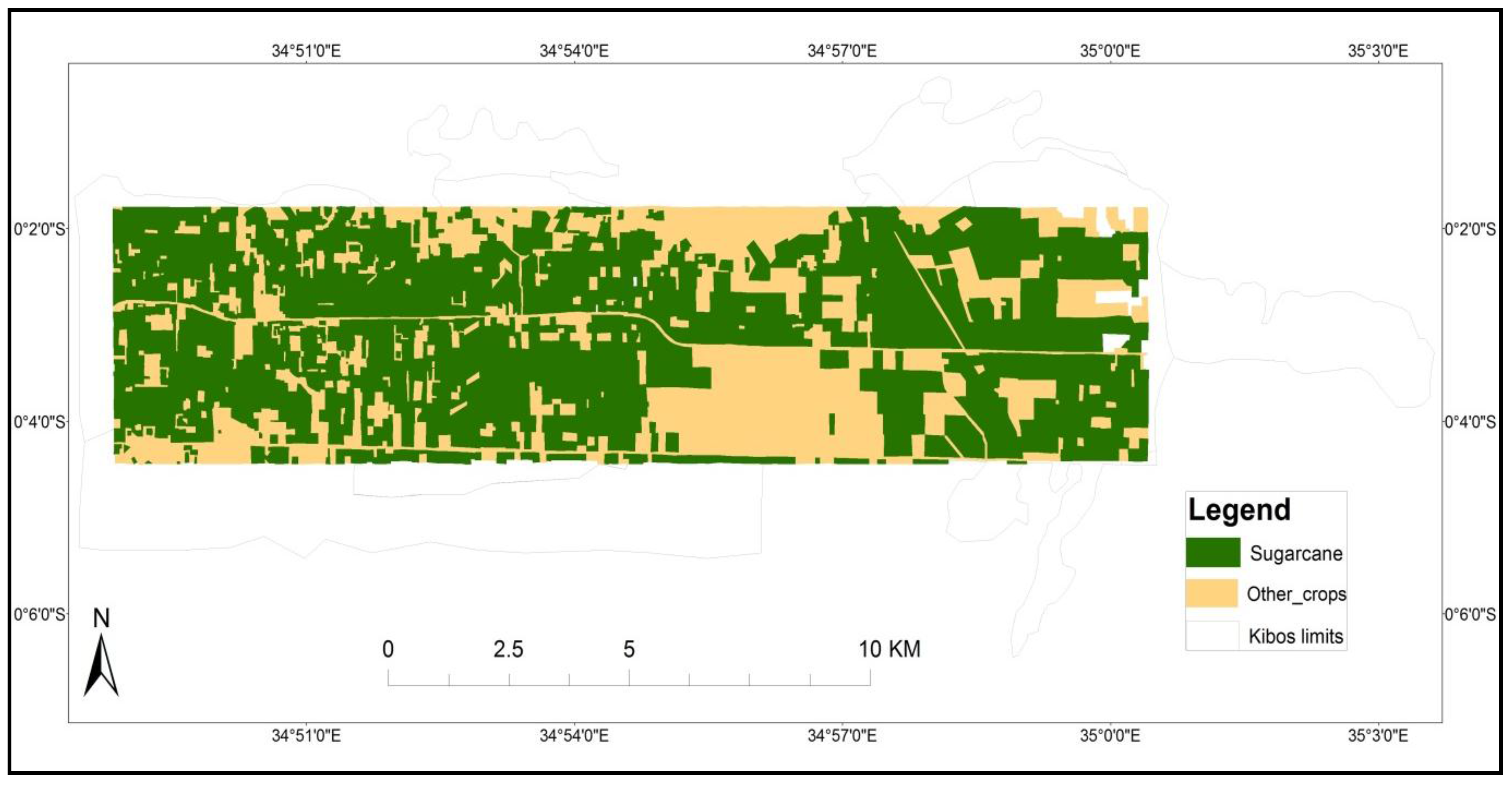
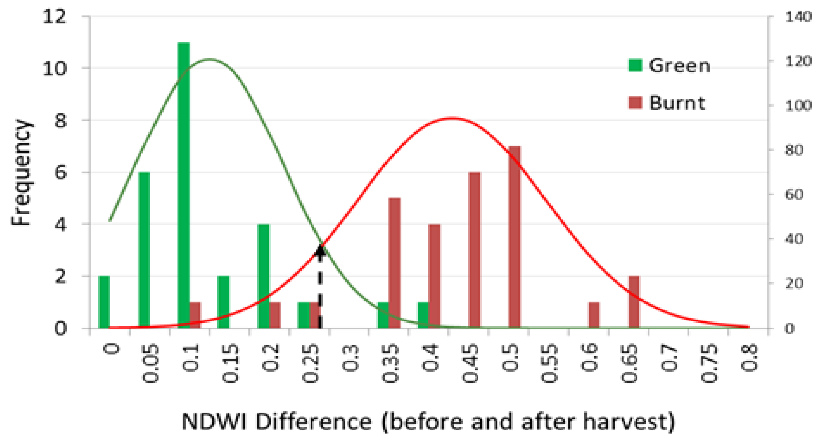
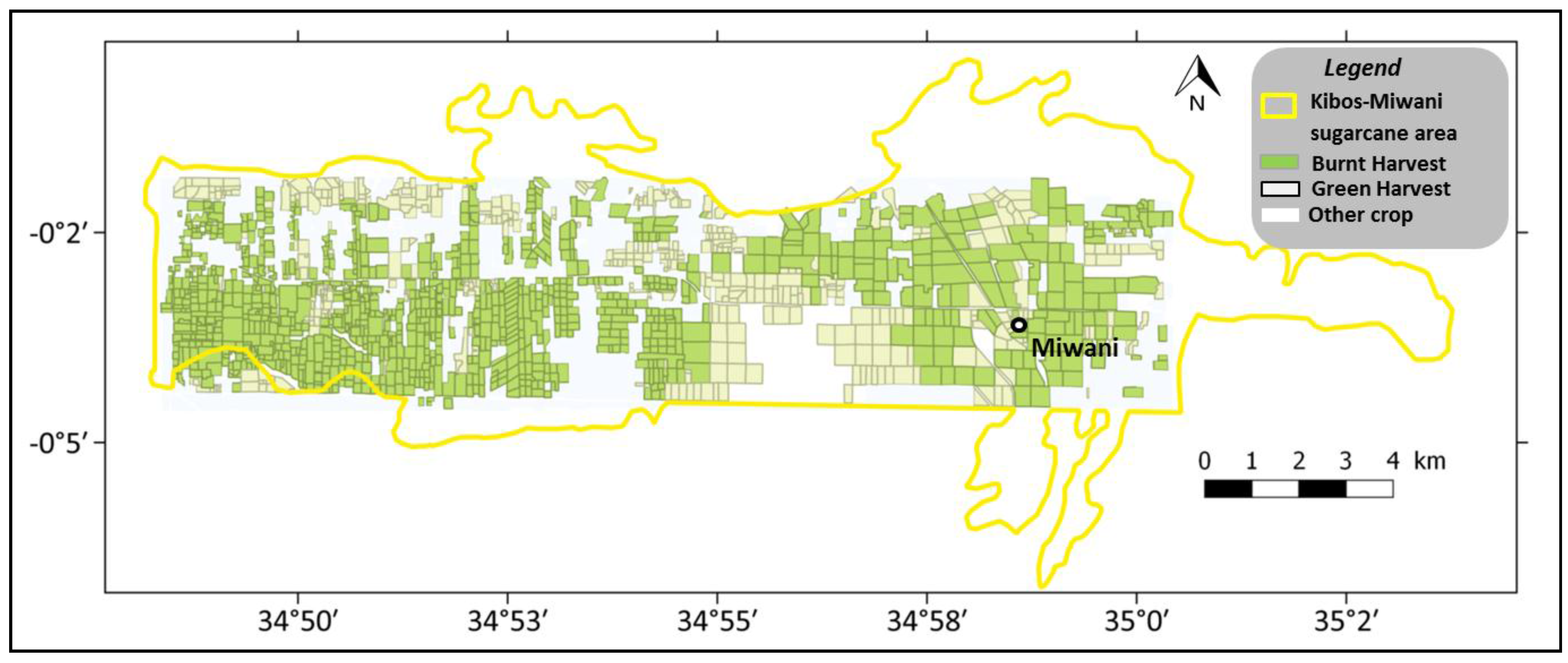
The harvest mode map was obtained using an original method through a t-test, which found Landsat normalized difference water index (NDWI) values for green and burnt harvest significantly different. NDWI distinguishes bare soil from vegetation residue after harvest by segregating dry and humid surfaces that result from burnt and green harvest respectively. Detection of harvest mode using NDWI is therefore a new idea, which this study has developed to characterize harvest mode. The harvest map will be used to plan for sensitization forums on best management and environmental practices.

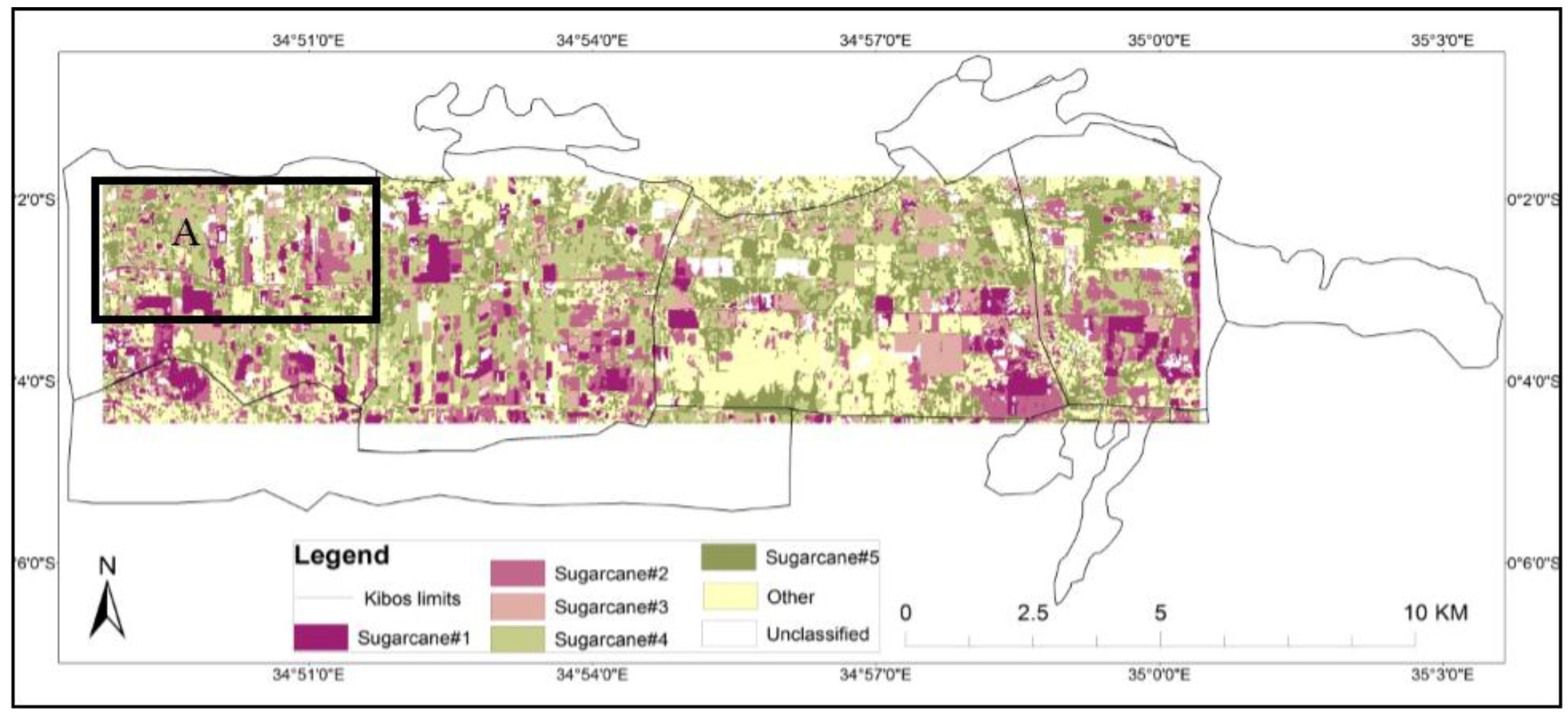
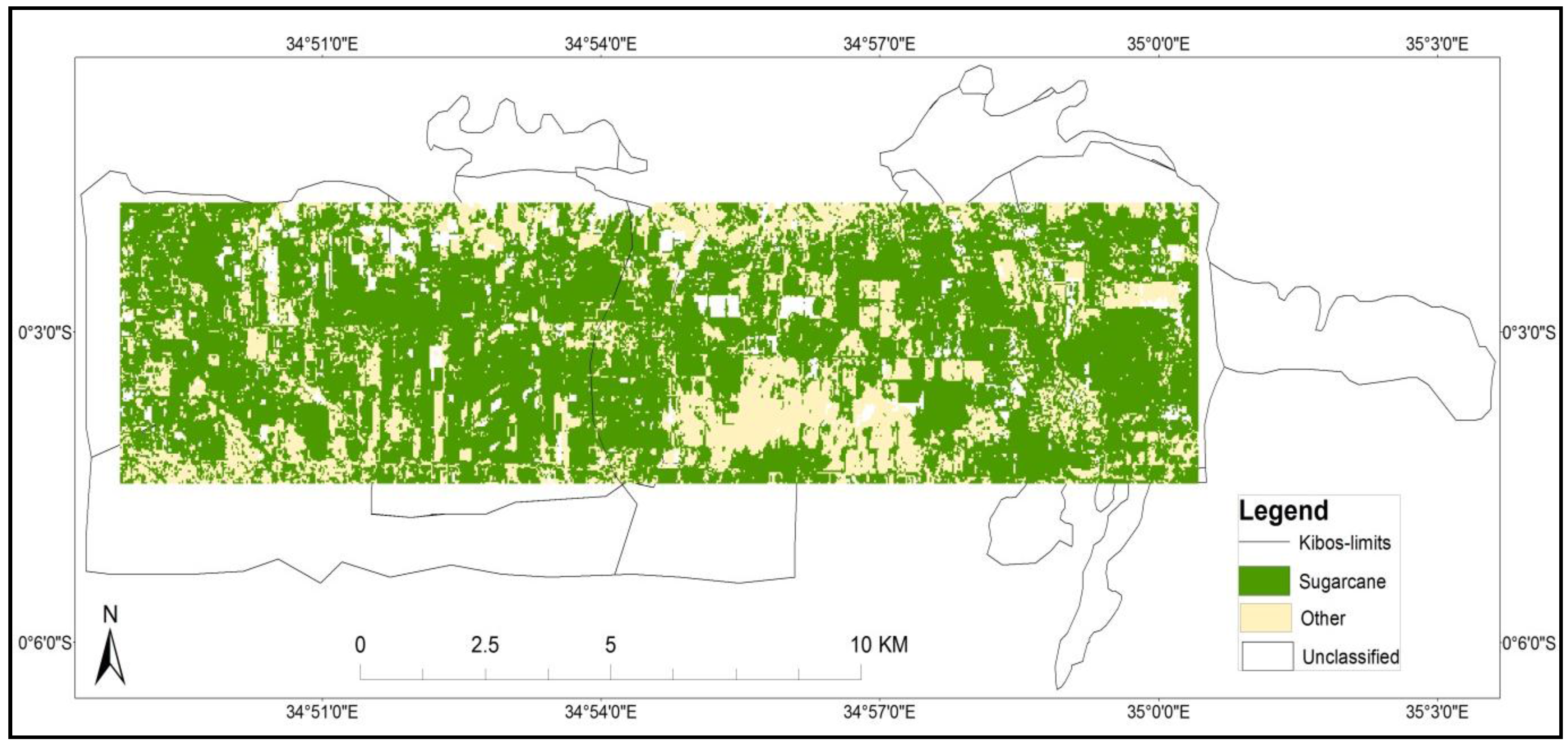
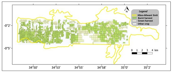
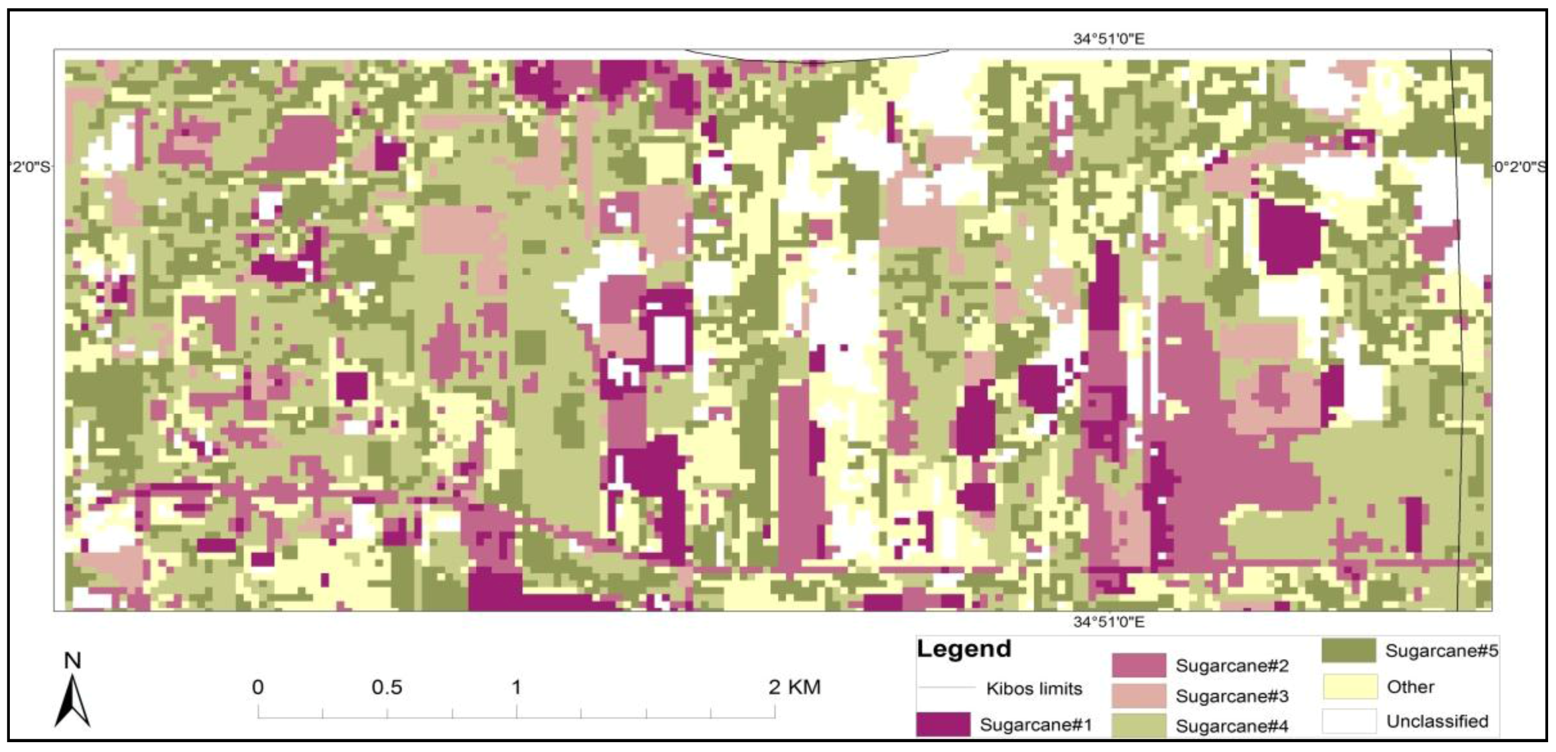
Moreover, Landsat NDVI has shown great potential for detecting crop type, crop conditions (harvested or growing) and mapping sugarcane cropped areas for medium sized farms over 1 ha in Kibos-Miwani. Farms that are less than 1 ha are however difficult to map at this image scale (15–30 m). The sugarcane map prepared in this study will be used as basis for precise acreages for increased accuracy in yield forecasting. To date, yield forecasting has been based on the Stack processed/planted Area regardless of where such field is located. The method developed in this study emphasizes on yield in a geographical zonation by remote sensing. Precise measurements will inform better planning decisions for the sugar industry operations [20] towards environment-friendly management of production areas. Moreover, NDWI will be used in precise mapping of sugarcane harvest modes. In the past, efforts by the sugar Industry to dissuade farmers on burnt harvest mode in Kenya have been limited by lack of techniques in mapping the practice.

Recent Earth Observing satellite systems, such as Sentinel-2 (S2 ESA), with decametric spatial resolution, and a high visiting frequency (10 days in 2015, and 5 days in 2016), will give access to farm level information. This S2 ESA satellite mission will also benefit for sugarcane mapping that is presently done using Landsat time series, with a resolution that is able to capture boundaries of nucleus fields, but not for small growers.

References

1. Araujo-Barbosa, C.C.; Atkinson, P.M.; Dearing, J.A. Remote sensing of ecosystem services: A systematic review. Ecol. Indic. 2015, 52, 430–443. [Google Scholar] [CrossRef]
2. Robertson, G.P.; Eldor, P.; Harwood, R. Greenhouse gases in intensive agriculture: Contributions of individual gases to the radiative forcing of the atmosphere. Science 2000, 289, 922–925. [Google Scholar] [CrossRef]
3. South, S.; Qi, J.; Lusch, D.P. Optimal classification methods for mapping agricultural tillage practices. Remote Sens. Environ. 2004, 91, 90–97. [Google Scholar] [CrossRef]
4. Razafimbelo, T.; Barthès, B.; Larré-Larrouy, M.C.; de-Luca, E.; Laurent, J.Y.; Cerri, C.C.; Feller, C. Effect of sugarcane residue management (mulching versus burning) on organic matter in a clayey Oxisol from southern Brazil. Agric. Ecosyst. Environ. 2006, 115, 285–289. [Google Scholar] [CrossRef]
5. De-Figueiredo, E.B.; la-Scala, J.N. Greenhouse gas balance due to the conversion of sugarcane areas from burned to green harvest in Brazil. Agric. Ecosyst. Environ. 2001, 141, 77–85. [Google Scholar] [CrossRef]
6. Panosso, A.R.; Marques, J.J.; Milori, D.M.B.P.; Ferraudo, A.S.; Barbieri, D.M.; Pereira, G.T.; La-Scala, J.N. Soil CO2 emission and its relation to soil properties in sugarcane areas under slash-and-burn and green harvest. Soil Tillage Res. 2011, 111, 190–196. [Google Scholar] [CrossRef]
7. Jamoza, J.E.; Amolo, R.A.; Muturi, S.M. A Baseline Survey on the Status of Sugarcane Production Technologies in Western Kenya; International Society of Sugar Cane Technologists: Sao Paulo, Brazil, 2013. [Google Scholar]
8. KSB. Year Book of Statistics; Kenya Sugar Board: Nairobi, Kenya, 2012. [Google Scholar]
9. Mulianga, B.; Bégué, A.; Simoes, M.; Todoroff, P. Forecasting regional sugarcane yield based on time integral and spatial aggregation of MODIS NDVI. Remote Sens. 2013, 5, 2184–2199. [Google Scholar] [CrossRef] [Green Version]
10. Blaschke, M.T. Object based image analysis for remote sensing. ISPRS J. Photogram. Remote Sens. 2010, 65, 2–16. [Google Scholar] [CrossRef]
11. Pettorelli, N.; Vik, J.O.; Mysterud, A.; Gaillard, J.M.; Tucker, C.J.; Stenseth, N.C. Using the satellite-derived NDVI to assess ecological responses to environmental change. Trends Ecol. Evol. 2005, 20, 503–510. [Google Scholar] [CrossRef] [PubMed]
12. Longley, P.A.; Goodchild, M.F.; Maguire, D.J.; Rhind, D.W. Geographical Information Systems: Principles, Techniques, Management, and Applications; John Wiley & Sons, Inc.: Hoboken, NJ, USA, 2005. [Google Scholar]
13. Begue, A.; Lebourgeois, V.; Bappel, E.; Todoroff, P.; Pellegrino, A.; Baillarin, F.; Siegmund, B. Spatio-temporal variability of sugarcane fields and recommendations for yield forecast using NDVI. Int. J. Remote Sens. 2010, 31, 5391–5407. [Google Scholar] [CrossRef] [Green Version]
14. Rudorff, B.F.T.; Aguiar, D.A.; Silva, W.F.; Sugawara, L.M.; Adami, M.; Moreira, M.A. Studies on the rapid expansion of sugarcane for ethanol production in São Paulo State (Brazil) using Landsat data. Remote Sens. 2010, 2, 1057–1076. [Google Scholar] [CrossRef]
15. El-Hajj, M.; Bégué, A.; Guillaume, S.; Martiné, J.-F. Integrating SPOT-5 time series, crop growth modeling and expert knowledge for monitoring agricultural practices: The case of sugarcane harvest on Reunion Island. Remote Sens. Environ. 2009, 113, 2052–2061. [Google Scholar] [CrossRef]
16. Vieira, M.A.; Formaggio, A.R.; Rennó, C.D.; Atzberger, C.; Aguiar, D.A.; Mello, M.P. Object based image analysis and data mining applied to a remotely sensed Landsat time-series to map sugarcane over large areas. Remote Sens.Environ. 2012, 123, 553–562. [Google Scholar] [CrossRef]
17. Thenkabail, P.S.; Wu, Z. An Automated Cropland Classification Algorithm (ACCA) for Tajikistan by combining Landsat, MODIS, and secondary data. Remote Sens. 2012, 4, 2890–2918. [Google Scholar] [CrossRef]
18. Mulianga, B.; Bégué, A.; Simoes, M.; Todoroff, P.; Clouvel, P. MODIS data for forecasting sugarcane yield in Kenya through a zonal approach. In Proceedings of the Sentinel-2 Preparatory Symposium, Frascati, Italy, 23–27 April 2012.
19. Amolo, R.; Abayo, G.; Muturi, S.; Rono, J. The Impact of Planting and Harvesting Time on Sugarcane Productivity in Kenyan Sugar Industry; KESREF: Kisumu, Kenya, 2009; pp. 18–27. [Google Scholar]
20. Mulianga, B. Assessing spatial heterogeneity and temporal dynamics of sugarcane landscape in western Kenya by remote sensing: Implications for environmental services. Availavble online: http://agritrop.cirad.fr/574730/ (accessed on 1 October 2015).
21. KSB. Year Book of Statistics; Kenya Sugar Board: Nairobi, Kenya, 2010. [Google Scholar]
22. Monroy, L.; Mulinge, W.; Witwer, M. Analysis of Incentives and Disincentives for Sugar in Kenya; Technical Notes Series, MAFAP; FAO: Rome, Italy, 2012. [Google Scholar]
23. Aguiar, D.A.; Friedrich, B.; Rudorff, T.; Silva, W.F.; Adami, M.; Mello, M.P. Remote sensing images in support of environmental protocol: Monitoring the sugarcane harvest in Sao Paulo State, Brazil. Remote Sens. 2011, 3, 2682–2703. [Google Scholar] [CrossRef]
24. Lebourgeois, V.; Begue, A.; Degenne, P.; Bappel, E. Improving harvest and planting monitoring for smallholders with geospatial technology: The Reunion Island experience. Int. Sugar J. 2010, 1298, 109–119. [Google Scholar]
25. Shisanya, C.; Recha, C.; Anyamba, A. Rainfall variability and its impact on normalized difference vegetation index in arid and semi-arid lands of Kenya. Int. J. Geosci. 2012, 2, 36–47. [Google Scholar] [CrossRef]
26. Cochran, W.G. Sampling Techniques, 3rd ed.; John Wiley and Sons: New York, NY, USA, 1977. [Google Scholar]
27. Rouse, J.W. Monitoring the Vernal Advancement of Retrogradation of Natural Vegetation; Type III, Final Report; NASA/GSFC: Greenbelt, MD, USA, 1974. [Google Scholar]
28. Gao, B. NDWI, a normalized difference water index for remote sensing of vegetation liquid water from space. Remote Sens. Environ. 1996, 58, 257–266. [Google Scholar] [CrossRef]
29. Gu, Y.; Hunt, E.; Wardlow, B.; Basara, J.B.; Brown, J.F.; Verdin, J.P. Evaluation of MODIS NDVI and NDWI for vegetation drought monitoring using Oklahoma Mesonet soil moisture data. Geophys. Res. Lett. 2008, 35. [Google Scholar] [CrossRef]
30. Wardlow, B.D.; Egbert, S.L. Large area crop mapping using time-series MODIS 250 m NDVI data: An assessment for the US Central Great Plains. Remote Sens. Environ. 2008, 112, 1096–1116. [Google Scholar] [CrossRef]
31. Congalton, R.G.; Green, K. Assessing the Accuracy of Remotely Sensed Data: Principles and Practices; CRC Press: Boca Raton, FL, USA, 1991. [Google Scholar]
32. Vintrou, E.; Desbrosse, A.; Bégué, A.; Traoré, S.; Baron, C.; Lo-Seen, D. Crop area mapping in West Africa using landscape stratification of MODIS time series and comparison with existing global land products. Int. J. Appl. Earth Obs. Geoinf. 2012, 14, 83–93. [Google Scholar] [CrossRef]
33. Zarco-Tejada, P.J.; Ustin, S.L.; Whiting, M.L. Temporal and spatial relationships between within-field yield variability in cotton and high-spatial hyperspectral remote sensing imagery. Agronomy J. 2005, 97, 641–653. [Google Scholar] [CrossRef]
34. Sader, S.A.; Bertrand, M.; Wilson, E.H. Satellite change detection of forest harvest patterns on an industrial forest landscape. For. Sci. 2003, 49, 341–353. [Google Scholar]
35. Chen, D.; Huang, J.; Jackson, T.J. Vegetation water content estimation for corn and soybeans using spectral indices derived from MODIS near- and short-wave infrared bands. Remote Sens. Environ. 2005, 98, 225–236. [Google Scholar] [CrossRef]
36. Todd, W.J.; Gehring, D.G.; Haman, J.F. Landsat wildland mapping accuracy. Photogram. Eng. Remote Sens. 1980, 46, 509–520. [Google Scholar]